DOI:10.32604/csse.2023.027377
| Computer Systems Science & Engineering DOI:10.32604/csse.2023.027377 | |
| Article |
Cat Swarm with Fuzzy Cognitive Maps for Automated Soil Classification
1Department of Computer Science and Information Systems, College of Applied Sciences, AlMaarefa University, Ad Diriyah, Riyadh, 13713, Kingdom of Saudi Arabia
2Department of Computer Engineering, College of Computers and Information Technology, Taif University, Taif, 21944, Kingdom of Saudi Arabia
3Department of Computing, Arabeast Colleges, Riyadh, 11583, Kingdom of Saudi Arabia
4Department of Archives and Communication, King Faisal University, Al Ahsa, Hofuf, 31982, Kingdom of Saudi Arabia
*Corresponding Author: Ashit Kumar Dutta. Email: drashitkumar@yahoo.com
Received: 16 January 2022; Accepted: 23 February 2022
Abstract: Accurate soil prediction is a vital parameter involved to decide appropriate crop, which is commonly carried out by the farmers. Designing an automated soil prediction tool helps to considerably improve the efficacy of the farmers. At the same time, fuzzy logic (FL) approaches can be used for the design of predictive models, particularly, Fuzzy Cognitive Maps (FCMs) have involved the concept of uncertainty representation and cognitive mapping. In other words, the FCM is an integration of the recurrent neural network (RNN) and FL involved in the knowledge engineering phase. In this aspect, this paper introduces effective fuzzy cognitive maps with cat swarm optimization for automated soil classification (FCMCSO-ASC) technique. The goal of the FCMCSO-ASC technique is to identify and categorize seven different types of soil. To accomplish this, the FCMCSO-ASC technique incorporates local diagonal extrema pattern (LDEP) as a feature extractor for producing a collection of feature vectors. In addition, the FCMCSO model is applied for soil classification and the weight values of the FCM model are optimally adjusted by the use of CSO algorithm. For examining the enhanced soil classification outcomes of the FCMCSO-ASC technique, a series of simulations were carried out on benchmark dataset and the experimental outcomes reported the enhanced performance of the FCMCSO-ASC technique over the recent techniques with maximum accuracy of 96.84%.
Keywords: Soil classification; intelligent models; fuzzy cognitive maps; cat swarm optimization; fuzzy logic
Soil plays a critical role in the global hydrologic cycle by governing the transmission of rainfall, surface runoff, and rate of infiltration, that is, precipitation that doesn't infiltrate the soil and run over the land surface into water bodies, namely lakes, rivers, and streams. Runoff arises once the rainfall surpasses the infiltration capacity of soil, also it is depending on the land cover, physical nature of soils, vegetation, storm, and hillslope property includes rainfall intensity, amount, and duration [1]. The rainfall runoff procedure has served as a catalyst for transporting contaminants and sediment, for example, pesticides, fertilizers, organic matter, and chemicals, adversely affecting the biodiversity and morphology of receiving water bodies [2]. Erosion and Flooding caused by uncontrollable runoff, especially down-stream, causes damage to manmade structures and agricultural land [3]. Therefore, modeling surface runoff is a crucial part of water and soil conservation effort includes but has not been limited to, monitoring soil and water quality and soil erosion, and forecasting floods. Soil can be categorized as sandy clay, clayey sand, clay, silty sand, clayey peat, peat, and humus clay. Several soil classification models are existing in the study. The signal and boundary energy model for extracting features [4]. Further, several classifications such as decision tree (DT), support vector machine (SVM), and artificial neural network (ANN) are utilized. In general, cone penetration test (CPT) is the traditional soil examination method that examines the deep knowledge and sub-surface of soil and sample [5]. In case of CPT that result the overlapping of different kinds of soil includes the soil composition relation and the mechanical behavior of soil is often uncertain [6]. Furthermore, Gordon studies the efficacy of SVM classification for image-based soil classification. Generally, the efficiency of classification can be impacted by the relevance of extracted feature. Several feature extraction techniques were proposed for soil image classification that is classified as; statistics-and learning-based processes [7]. In learning-based process, feature of image is extracted by utilizing different machine learning (ML) methods.
In order to prevent misclassification resulting from subjective coincidence, [8] proposed a smart technique for providing the nearest value of the Munsell chips to unknown colour of soil samples by utilizing FL and ANN algorithms. Shivhare et al. [9] proposed an approach for classifying the soil at its better efforts by extracting the feature. The presented method makes use of Gabor Wavelet and SVM for classifying better recommendations and for recognizing soil type. The aim is to handle the soil picture to transport a higher-level soil classifier for rustic ranchers at low-cost.
Rahman et al. [10] developed an approach which could forecast soil series using land types and based on the estimation it could recommend appropriate crops. Various ML methods namely Gaussian kernel based SVM, weighted k-nearest neighbor (KNN), and Bagged Trees are utilized for classifying soils. The experiment result shows that our presented SVM based approach is effectively performed when compared to several current methodologies. In Gambill et al. [11], random forest (RF)-ML method has been utilized for creating a USCS predictive method with USDA soil property variable. Significant variables to predict USCS code from available soil property are available water storage, USDA soil textures, and percent organic material.
Khullar et al. [12], proposed an efficient and appropriate soil classification method to implement DL methods. Image-based soil dataset was pre-processed and collected based on algorithmic requirements. At first, classification has been carried by utilizing ML classification method and compared to DL models. Abraham et al. [13] introduce an application of ML for classifying soil into hydrologic groups. According to the feature includes percentage of silt, clay, and sand, and the values of saturated hydraulic conductivity, ML algorithms have been trained to categorize soil into 4 hydrologic classes. The classification outcomes attained by utilizing approaches like KNN, Classification Bagged Ensembles, DT, TreeBagger, and SVM with Gaussian Kernel have been compared to soil texture.
This paper introduces effective fuzzy cognitive maps with cat swarm optimization for automated soil classification (FCMCSO-ASC) technique. The goal of the FCMCSO-ASC technique is to identify and categorize seven different types of soil. To accomplish this, the FCMCSO-ASC technique incorporates local diagonal extrema pattern (LDEP) as a feature extractor for producing a collection of feature vectors. In addition, the FCMCSO model is applied for soil classification and the weight values of the FCM model are optimally adjusted by the use of CSO algorithm. For examining the enhanced soil classification outcomes of the FCMCSO-ASC technique, a series of simulations were carried out on benchmark dataset.
This paper has developed a novel FCMCSO-ASC technique to identify and categorize seven different types of soil. The FCMCSO-ASC technique incorporates different processes namely data augmentation, LDEP based feature extraction, FCM based classification, and CSO based parameter optimization. Here, the FCMCSO model is applied for soil classification and the weight values of the FCM model are optimally adjusted by the use of CSO algorithm.
2.1 Feature Extraction Using LDEP Technique
At the initial stage, the LDEP technique receives the soil images as input and generates corresponding feature vectors. LDEP is a novel image feature description presented by Dubey et al. [14] to CT image retrievals. The LDEP encoded the connection of central pixels with their local diagonal neighbor. To provide central pixels, LDEP defines their local diagonal extrema (maximum and minimum) utilizing 1st-order local diagonal derivative. Afterward, these attained local diagonal extrema were encoded for forming the LDEP patterns to respective central pixels. The LDEP pattern to some pixels (k, l) was provided as:
where dim refers the length of LDEP patterns and LDEP k, l is jth component of LDEP pattern of pixels
where
where
where
where
2.2 Soil Classification Using FCM Model
Next to the feature extraction process, the classification process is carried out using the FCM model, to identify the different types of soil. FCMs are realized as RNNs with interpretability features which are extremely utilized from modeling tasks [16]. It can contain group of neural processing entities named concept (neuron) and its causal relation. The activation value of such neurons regularly proceeds values from the zero and one interval, thus the stronger the activation value of neurons, the superior to their influence on the networks. Obviously, the linked weight is also appropriate during this method. The strength of causal connection amongst 2 neurons Ci and Cj has quantified by numerical weight wij ∈ [ − 1, 1] and represented using a causal edge in Ci to
– When wij > 0 then higher (decrement) from the reason Ci generates a raise (decrement) of effects Cj with intensity |wij|.
– Once wij < 0 then an enhance (decrement) from the reason Ci takes a decrement (increment) of the neurons Cj with intensity |wij|.
– When wij = 0 then there is no causal connection amongst Ci and Cj. Eq. (7) illustrates Kosko's activation rule, with A(0) being the primary state. This rule was iteratively repeating still end criteria is met. A novel activation vector was computed at all steps t and then a set amount of iterations, the FCM shall be at most subsequent states: (1) equilibrium point, (2) limited cycle, or (3) chaotic performance. The FCM was supposed that have met when it attains fixed-point attractors, else the upgrade method ends then a maximal count of iterations T was attained.
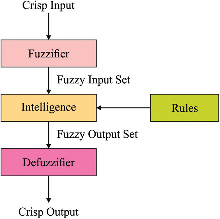
Figure 1: Fuzzy logic
The function f( ⋅ ) in Eq. (7) refers the monotonically non-decrease nonlinear function utilized for clamping the activation value of all neurons to permitted interval. Instances of such functions as sigmoid variants, bivalent function, and trivalent function. The focus on the sigmoid function as it has displayed higher prediction capability. Eq. (8) validates the nonlinear transfer function utilized in conducted research, in which λ denotes the sigmoid slope and h indicates the offset. Such parameters were closely compared to the network convergence.
Eq. (7) illustrates the inference rule extremely utilized from several FCM based applications, however, it could not the only one. The changed inference rule, initiate at Eq. (9), in which neurons get to account for their individual past values [17]. This rule was desired if upgrading the activation value of neurons which are not inclined by another neural processing entity.
Another altered upgrade rule for avoiding the conflict emerging from the case of non-active neurons. Most clearly, the rescaled inference demonstrated in Eq. (10) permits controlling the condition in which there is no data on primary neuron-state and uses avoiding the saturation problems. The reader is noticeable achieve the same effects by utilizing a shifted sigmoid function with adequate slopes.
When the cognitive network was capable of converging, afterward the system takes a similar output nearby the end, and so the activation degree of neurons are continue unchanged (or subject to infinitesimal change). Conversely, the cyclic FCM gets dissimilar responses with exception of some conditions that are periodically created. The final feasible condition was compared with chaotic configuration in that the network takes various state vectors.
2.3 Parameter Tuning Using CSO Algorithm
In order to properly adjust the weight values of the FCM model, the CSO algorithm can be employed to it. The CSO [18] is a comparatively novel stochastic, population based, metaheuristic evolutionary technique. CSO simulates 2 natural performances of cats, for instance, exploring their environment to their next move and tracing the target. The cat has a strong concern about nearby moving objects and excellent hunting skills. It is continuously stay alerted also during at rest. A significant type of cat is that it spends most often time from inertia and preserves its energy to future chases. In normal time its drive is also extremely slow. Once it senses a prey it can chase quickly spend massive count of energy. The CSO signifies the 2 performances; rest with slow movement and chase with maximum speed as well as energy as seek and trace modes. The soaring speed from seeking process was mathematically mapped as huge variation from their place.
Seeking mode
The 5 operators are there from seeking methods such as Counts of Dimension to Change (CDC), Mixture Ratio (MR), Seeking Memory Pool (SMP), Self-Position Consideration (SPC), and Seeking Range of Selected Dimension (SRD). In SMP explains the pool size of seeking memory or count of copies of the cat created i.e., when the value of SMP was set as 10 then all the cats are fit for storing 10 solutions set as candidates. The SRD was utilized for stating the mutative portions to chosen dimensional i.e., once a dimensional was chosen to mutation, the variance amongst the old as well as new values cannot be out of ranges. The CDC relates to the amount of dimensions that are altered from the seeking procedure.
The SPC is a Boolean value and when it can be true, one place in the memory is to store the existing solutions set and not be altered. The MR is a minimal value, for instance, fraction of populations was utilized for guaranteeing that cat spends amount of time from seeking method.
Tracing mode
The tracing process was considerably related to local search technique of swarm from PSO technique. During this process, the cats trace targets with maximum energy by altering the places with their individual velocity. The place and velocity of ith cat from D dimension solution space was demonstrated as:
The global optimum place of cat swarm was demonstrated as:
Upgrade the velocity and place of the existing cat utilizing in Eqs. (14) and (15)
where w refers the inertia weights, c1 signifies the acceleration constants and r1 stands for the arbitrary number uniformly distributed from the range of zero and one. The huge inertia weight enables a global search but lesser inertia weight helps a local search. During this case, w is fixed as 0.4. The cat swarm signifies the group of indices [19]. Utilizing these indices, equivalent decreased feature subset was derivative in the novel data set. It can occur that at time of selection more than one count of indices could not fall in the range of columns existing on that specific data set. The subsequent equation was implemented for selecting all novel index values in the range of columns.
if
else
In order to obtain one of the better candidate features with optimum classifier accuracy, altered CSO was executed for each data set.
For experimental validation, we have collected a set of ten images from various sources under seven classes namely Clayey sand, Sandy clay, Silty sand, Clay, Humus clay, Clayey peat, and Peat. To increase the number of images in the dataset, data augmentation process is carried out and the number of images becomes 30 after the data augmentation process. A few sample images are illustrated in Fig. 2.
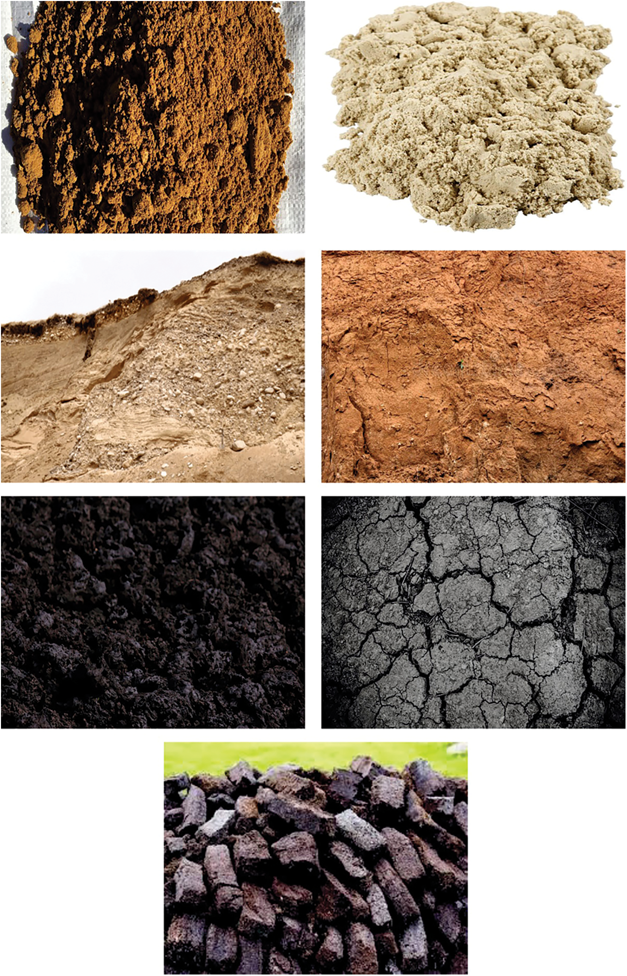
Figure 2: Sample images
The confusion matrix generated by the FCMCSO-ASC technique on the classification of soil under run-1 is depicted in Fig. 3. The results indicated that the FCMCSO-ASC technique has recognized 29 images into Clayey sand, 34 images into Sandy clay, 30 images into Silty sand, 31 images into Clay, 31 images into Humus clay, 38 images into Clayey peat, and 30 images into peat.
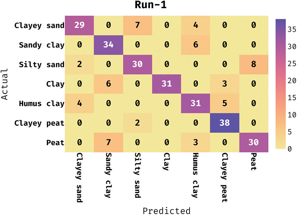
Figure 3: Confusion matrix analysis of FCMCSO-ASC technique under run-1
The classifier results obtained by the FCMCSO-ASC technique on the classification of soil into distinct classes under run-1 are reported in Tab. 1. The attained table values reported the improved soil classification results under all classes. For instance, the FCMCSO-ASC technique has identified the Clayey sand class with the precn, recal, accuy, and Fscore of 82.86%, 72.50%, 93.93%, and 77.33% respectively. Moreover, the FCMCSO-ASC technique has categorized the images into Sandy clay class with the precn, recal, accuy, and Fscore of 72.34%, 85%, 93.21%, and 77.33% respectively.
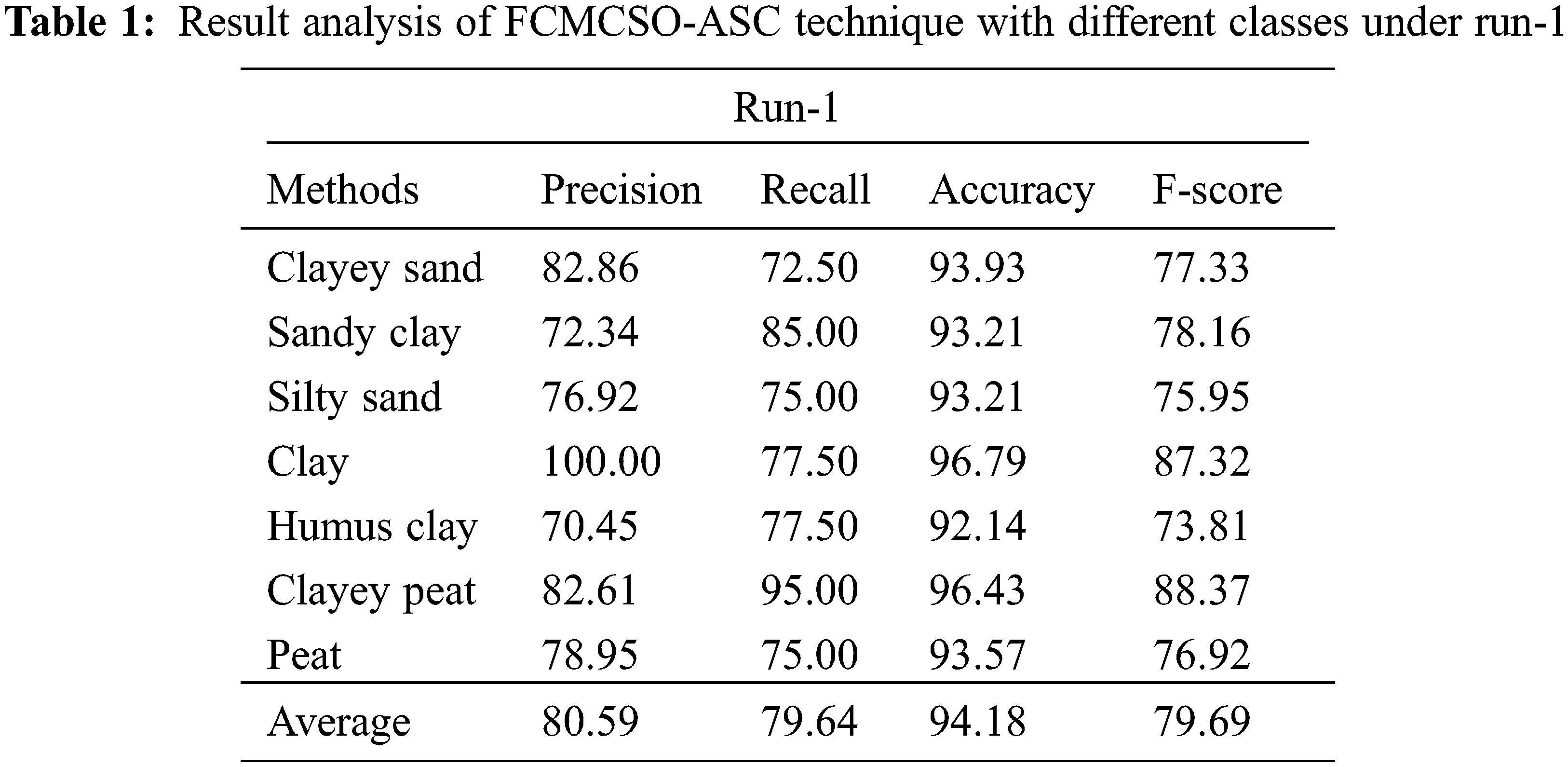
Fig. 4 illustrates the average soil classification results offered by the FCMCSO-ASC technique under run-1. The figure indicated that the FCMCSO-ASC technique has accomplished better performance with the average precn, recal, accuy, and Fscore of 80.59%, 79.64%, 94.18%, and 79.69% respectively.
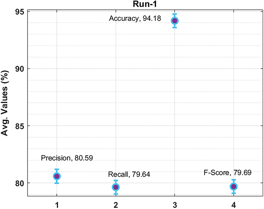
Figure 4: Average analysis of FCMCSO-ASC technique under run-1
The confusion matrix generated by the FCMCSO-ASC approach on the classification of soil under run-2 is illustrated in Fig. 5. The outcomes showed that the FCMCSO-ASC method has recognized 35 images into Clayey sand, 37 images into Sandy clay, 36 images into Silty sand, 33 images into Clay, 33 images into Humus clay, 38 images into Clayey peat, and 37 images into peat.
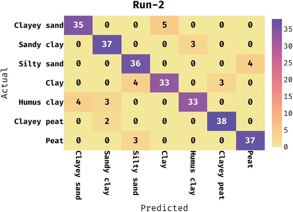
Figure 5: Confusion matrix analysis of FCMCSO-ASC technique under run-2
The classifier outcomes attained by the FCMCSO-ASC methodology on the classification of soil into various classes under run-2 are reported in Tab. 2. The obtained table values reported the enhanced soil classification results under all classes. For sample, the FCMCSO-ASC approach has identified the Clayey sand class with precn, recal, accuy, and Fscore of 89.74%, 87.50%, 96.79%, and 88.61% correspondingly. Eventually, the FCMCSO-ASC system has categorized the images into Sandy clay class with precn, recal, accuy, and Fscore of 88.10%, 92.50%, 97.14%, and 90.24% correspondingly.
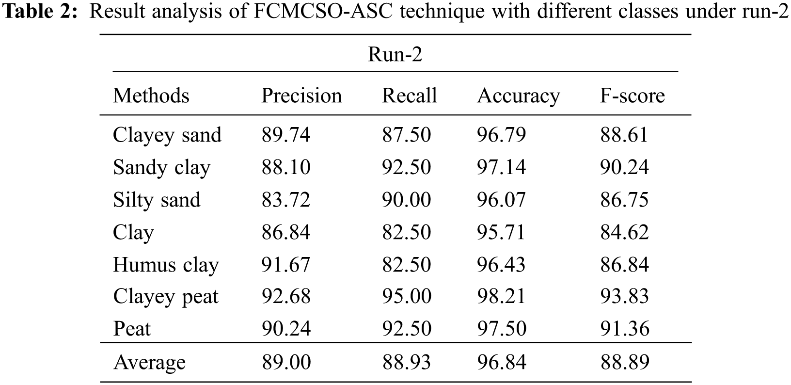
Fig. 6 depicts the average soil classification outcomes offered by the FCMCSO-ASC approach under run-2. The figure revealed that the FCMCSO-ASC methodology has accomplished better performance with the average precn, recal, accuy, and Fscore of 89%, 88.93%, 96.84%, and 88.89% correspondingly.
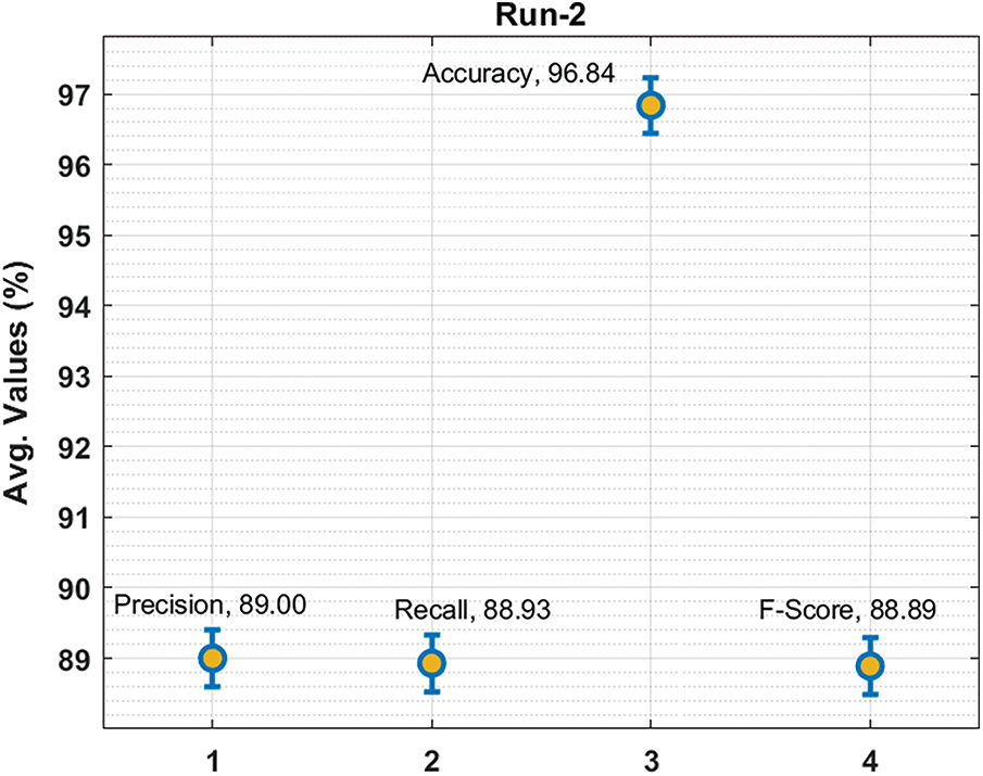
Figure 6: Average analysis of FCMCSO-ASC technique under run-2
In order to highlight the enhanced outcomes of the FCMCSO-ASC technique, a comparison study with existing techniques takes place in Tab. 3 [20]. Fig. 7 offers the comparative precn analysis of the FCMCSO-ASC technique with existing approaches. The figure reported that the particle swarm optimization (PSO), gravitational search algorithm (GSA), differential evolution (DE), and spider monkey optimization (SMO) techniques have resulted in reduced precn values of 76.29%, 76.46%, 76.56%, and 76.93% respectively. Followed by, the chaotic SMO (CSMO) technique has reached moderately improved classification results with precn of 80.80%. However, the FCMCSO-ASC technique has outperformed the other methods with the increased precn pf 89%.
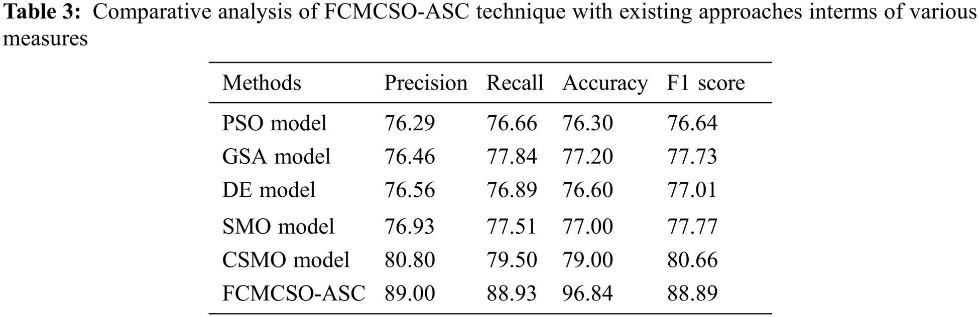
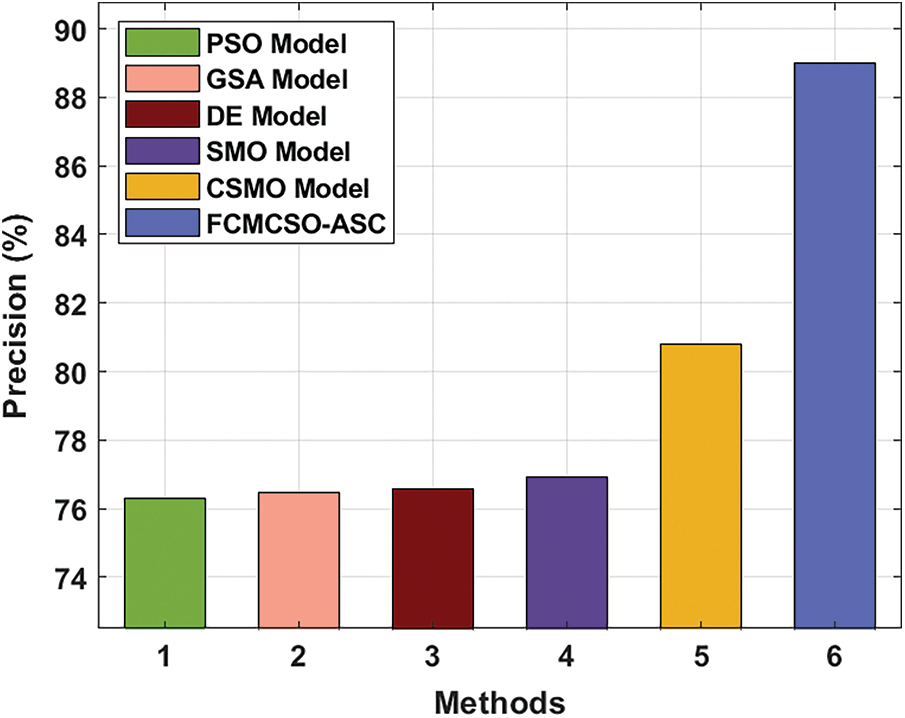
Figure 7: Precn analysis of FCMCSO-ASC technique with existing approaches
Fig. 8 provides the comparative recal analysis of the FCMCSO-ASC approach with existing methods. The figure stated that the PSO, GSA, DE, and SMO systems have resulted to lower recal values of 76.66%, 77.84%, 76.89%, and 77.51% correspondingly. Then, the CSMO technique has reached moderately enhanced classification results with recal of 79.50%. But, the FCMCSO-ASC methodology has demonstrated the other methods with the maximum recal pf 88.93%.
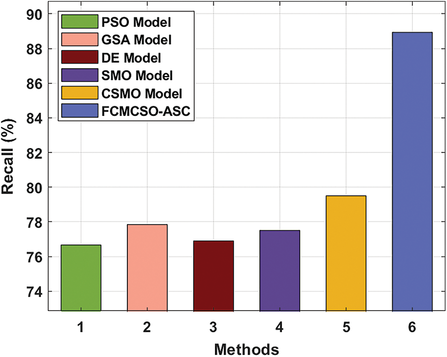
Figure 8: Recal analysis of FCMCSO-ASC technique with existing methods
Fig. 9 demonstrates the comparative accy analysis of the FCMCSO-ASC technique with existing approaches. The figure reported that the PSO, GSA, DE, and SMO techniques have resulted in reduced accy values of 76.30%, 77.20%, 76.60%, and 77% respectively. Afterward, the CSMO system has reached moderately improved classification results with accy of 79%. Finally, the FCMCSO-ASC technique has portrayed the other techniques with the increased accy of 96.84%.
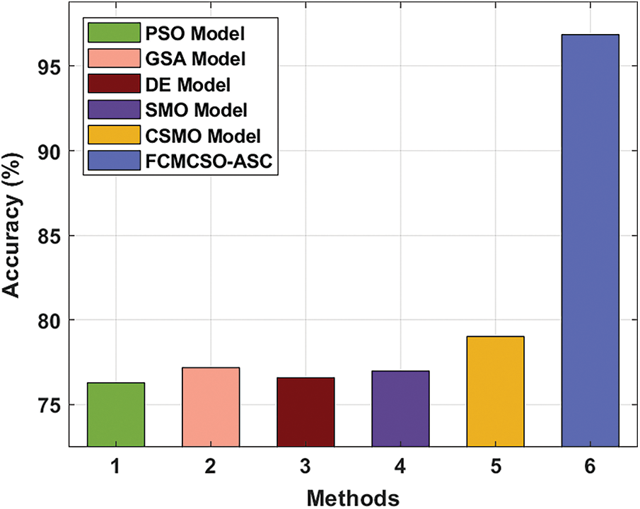
Figure 9: Accy analysis of FCMCSO-ASC technique with existing approaches
Finally, Fig. 10 showcases the comparative F1score analysis of the FCMCSO-ASC technique with existing approaches. The figure described that the PSO, GSA, DE, and SMO methodologies have resulted in reduced F1score values of 76.64%, 77.73%, 77.01%, and 77.77% respectively. Similarly, the CSMO approach has obtained moderately increased classification results with F1score of 80.66%. At last, the FCMCSO-ASC technique has exhibited the other methods with the increased F1score pf 88.89%.
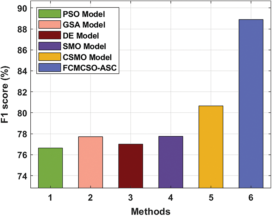
Figure 10: F1score analysis of FCMCSO-ASC technique with existing approaches
This paper has developed a novel FCMCSO-ASC technique to identify and categorize seven different types of soil. The FCMCSO-ASC technique incorporates different processes namely LDEP based feature extraction, FCM based classification, and CSO based parameter optimization. Here, the FCMCSO model is applied for soil classification and the weight values of the FCM model are optimally adjusted by the use of CSO algorithm. For examining the enhanced soil classification outcomes of the FCMCSO-ASC technique, a series of simulations were carried out on benchmark dataset and the experimental outcomes reported the enhanced performance of the FCMCSO-ASC technique over the recent techniques. Therefore, the FCMCSO-ASC technique can be applied as an effective tool for automated soil classification. As a part of future scope, the soil classification outcomes of the FCMCSO-ASC technique can be improvised by the deep learning models.
Acknowledgement: The authors deeply acknowledge the Researchers supporting program (TUMA-Project-2021-27) Almaarefa University, Riyadh, Saudi Arabia for supporting steps of this work.
Funding Statement: This research was supported by the Researchers Supporting Program (TUMA-Project-2021-27) Almaarefa University, Riyadh, Saudi Arabia. Taif University Researchers Supporting Project Number (TURSP-2020/161), Taif University, Taif, Saudi Arabia.
Conflicts of Interest: The authors declare that they have no conflicts of interest to report regarding the present study.
1. K. Srunitha and S. Padmavathi, “Performance of SVM classifier for image based soil classification,” in 2016 Int. Conf. on Signal Processing, Communication, Power and Embedded System (SCOPES), Paralakhemundi, Odisha, India, pp. 411–415, 2016. [Google Scholar]
2. B. Bhattacharya and D. P. Solomatine, “Machine learning in soil classification,” Neural Networks, vol. 19, no. 2, pp. 186–195, 2006. [Google Scholar]
3. R. Shenbagavalli, “Classification of soil textures based on laws features extracted from preprocessing images on sequential and random windows,” Bonfring International Journal of Advances in Image Processing, vol. 1, no. 1, pp. 15–18, 2011. [Google Scholar]
4. M. Saraswat and K. V. Arya, “Feature selection and classification of leukocytes using random forest,” Medical & Biological Engineering & Computing, vol. 52, no. 12, pp. 1041–1052, 2014. [Google Scholar]
5. J. K. Kumar, M. Konno and N. Yasuda, “Subsurface soil-geology interpolation using fuzzy neural network,” Journal of Geotechnical and Geoenvironmental Engineering, vol. 126, no. 7, pp. 632–639, 2000. [Google Scholar]
6. M. v. Rooyen, N. Luwes and E. Theron, “Automated soil classification and identification using machine vision,” in 2017 Pattern Recognition Association of South Africa and Robotics and Mechatronics (PRASA-RobMech), Bloemfontein, South Africa, pp. 249–252, 2017. [Google Scholar]
7. S. K. Lenka and A. G. Mohapatra, “Gradient descent with momentum based neural network pattern classification for the prediction of soil moisture content in precision agriculture,” in 2015 IEEE Int. Symp. on Nanoelectronic and Information Systems, Indore, India, pp. 63–66, 2015. [Google Scholar]
8. M. C. Pegalajar, L. G. B. Ruiz, M. S. Marañón and L. Mansilla, “A munsell colour-based approach for soil classification using fuzzy logic and artificial neural networks,” Fuzzy Sets and Systems, vol. 401, pp. 38–54, 2020. [Google Scholar]
9. S. Shivhare and K. Cecil, “Automatic soil classification by using gabor wavelet & support vector machine in digital image processing,” in 2021 Third Int. Conf. on Inventive Research in Computing Applications (ICIRCA), Coimbatore, India, pp. 1738–1743, 2021. [Google Scholar]
10. S. A. Z. Rahman, K. C. Mitra and S. M. M. Islam, “Soil classification using machine learning methods and crop suggestion based on soil series,” in 2018 21st Int. Conf. of Computer and Information Technology (ICCIT), Dhaka, Bangladesh, pp. 1–4, 2018. [Google Scholar]
11. D. R. Gambill, W. A. Wall, A. J. Fulton and H. R. Howard, “Predicting USCS soil classification from soil property variables using random forest,” Journal of Terramechanics, vol. 65, pp. 85–92, 2016. [Google Scholar]
12. V. Khullar, S. Ahuja, R. G. Tiwari and A. K. Agarwal, “Investigating efficacy of deep trained soil classification system with augmented data,” in 2021 9th Int. Conf. on Reliability, Infocom Technologies and Optimization (Trends and Future Directions) (ICRITO), Noida, India, pp. 1–5, 2021. [Google Scholar]
13. S. Abraham, C. Huynh and H. Vu, “Classification of soils into hydrologic groups using machine learning,” Data, vol. 5, no. 1, pp. 2, 2019. [Google Scholar]
14. S. R. Dubey, S. K. Singh and R. K. Singh, “Local diagonal extrema pattern: A new and efficient feature descriptor for CT image retrieval,” IEEE Signal Processing Letters, vol. 22, no. 9, pp. 1215–1219, 2015. [Google Scholar]
15. Y. Kumar, A. Aggarwal, S. Tiwari and K. Singh, “An efficient and robust approach for biomedical image retrieval using zernike moments,” Biomedical Signal Processing and Control, vol. 39, pp. 459–473, 2018. [Google Scholar]
16. B. Kosko, “Fuzzy cognitive maps,” International Journal of Man-Machine Studies, vol. 24, no. 1, pp. 65–75, 1986. [Google Scholar]
17. G. Nápoles, M. Espinosa, I. Grau and K. Vanhoof, “FCM expert: Software tool for scenario analysis and pattern classification based on fuzzy cognitive maps,” International Journal on Artificial Intelligence Tools, vol. 27, no. 7, pp. 1860010, 2018. [Google Scholar]
18. K. C. Lin, Y. H. Huang, J. C. Hung and Y. T. Lin, “Feature selection and parameter optimization of support vector machines based on modified cat swarm optimization,” International Journal of Distributed Sensor Networks, vol. 11, no. 7, pp. 365869, 2015. [Google Scholar]
19. P. Mohapatra, S. Chakravarty and P. K. Dash, “Microarray medical data classification using kernel ridge regression and modified cat swarm optimization based gene selection system,” Swarm and Evolutionary Computation, vol. 28, pp. 144–160, 2016. [Google Scholar]
20. S. Kumar, B. Sharma, V. K. Sharma and R. C. Poonia, “Automated soil prediction using bag-of-features and chaotic spider monkey optimization algorithm,” Evolutionary Intelligence, vol. 14, no. 2, pp. 293–304, 2021. [Google Scholar]
 | This work is licensed under a Creative Commons Attribution 4.0 International License, which permits unrestricted use, distribution, and reproduction in any medium, provided the original work is properly cited. |