Computer Systems Science & Engineering DOI:10.32604/csse.2023.027744
Article

An Optimized Deep-Learning-Based Low Power Approximate Multiplier Design

M. Usharani1,*, B. Sakthivel2, S. Gayathri Priya3, T. Nagalakshmi4 and J. Shirisha5

1Department of Electronics and Communication Engineering, Er.Perunal Manimekalai College of Engineering, Konneripalli, Hosur, 635117, India
2Department of Electronics and Communication Engineering, Pandian Saraswathi Yadav Engineering College, Sivagangai, Tamilnadu, 630561, India
3Department of Electronics and Communication Engineering, R.M.D Engineering College, Gummidipundi, Tamilnadu, 601206, India
4Department of Computer Science and Engineering, Koneru Lakshmaiah Education Foundation, Vaddeswaram, Guntur, 522502, India
5Department of Electronics and Communication Engineering, Malla Reddy Engineering College, Hyderabad, Telangana, 500015, India
*Corresponding Author: M. Usharani. Email: usharaniphd@gmail.com
Received: 24 January 2022; Accepted: 27 February 2022

Abstract: Approximate computing is a popular field for low power consumption that is used in several applications like image processing, video processing, multimedia and data mining. This Approximate computing is majorly performed with an arithmetic circuit particular with a multiplier. The multiplier is the most essential element used for approximate computing where the power consumption is majorly based on its performance. There are several researchers are worked on the approximate multiplier for power reduction for a few decades, but the design of low power approximate multiplier is not so easy. This seems a bigger challenge for digital industries to design an approximate multiplier with low power and minimum error rate with higher accuracy. To overcome these issues, the digital circuits are applied to the Deep Learning (DL) approaches for higher accuracy. In recent times, DL is the method that is used for higher learning and prediction accuracy in several fields. Therefore, the Long Short-Term Memory (LSTM) is a popular time series DL method is used in this work for approximate computing. To provide an optimal solution, the LSTM is combined with a meta-heuristics Jellyfish search optimisation technique to design an input aware deep learning-based approximate multiplier (DLAM). In this work, the jelly optimised LSTM model is used to enhance the error metrics performance of the Approximate multiplier. The optimal hyperparameters of the LSTM model are identified by jelly search optimisation. This fine-tuning is used to obtain an optimal solution to perform an LSTM with higher accuracy. The proposed pre-trained LSTM model is used to generate approximate design libraries for the different truncation levels as a function of area, delay, power and error metrics. The experimental results on an 8-bit multiplier with an image processing application shows that the proposed approximate computing multiplier achieved a superior area and power reduction with very good results on error rates.

Keywords: Deep learning; approximate multiplier; LSTM; jellyfish

1  Introduction

Recently, approximate computing is an emerging approach to reduce the power consumption for several applications like video processing, multimedia, image processing and data mining etc. The approximate computing technique is performed by regulating the inexact calculation with a tolerable error in terms of reducing power and increasing an operational frequency. These errors have not affected the operations of computing and its performances [1]. The performance of approximate computing is based on multiplication and additions. The function of multiplier or adder is truncated with some error compensation which consumes a low power than exact circuits. This inexact or approximate design of adder or multiplier will not affect a system’s output and it also improved energy efficiency with a good performance.

The Multipliers are the primary component in Approximate computing which is utilized for many applications like digital signal processors, microprocessors and embedded systems [2]. Also, multiplier requires high energy consumption and also design complexity. It becomes a greater challenge to design a low power multiplier in digital circuits. On designing approximate multipliers, performance in terms of energy consumption and hardware complexity is reduced. Thus the approximate multiplier application achieved higher success in research and also enhanced the quality and performance of systems. Though it is also more challenging to work for researchers in minimum power, the field is searching for a few implementations with a higher training of input dependent or input aware techniques.

The DL is an advanced learning technique for solving a complex issue and highly predictable than any other method. The DL model of Long Short-Term Memory (LSTM) model is used which is highly efficient in classifying, predicting and processing the data in time series [3]. The main contribution of the proposed work is to introduce a new DL model-based approximate multiplier with the awareness of prediction in area, delay and power for the corresponding truncation levels.

To enhance the optimal Accuracy in approximate computing, the LSTM is combined with a Meta-heuristics algorithm like the jellyfish Search Optimization algorithm. The jellyfish Search Optimization is based on swarm Meta-heuristics that is developed by its food searching behaviour in an ocean current. In this work, the novel input aware approximate multiplier design technique is presented. The input awareness is done by using a novel Jelly optimised LSTM technique that is used to pre-train the input data of the Approximate multiplier. This Approximate multiplier is highly trained with an optimal result and stored in a library. As a result, by implementing this input aware approximate multiplier, the performance of approximate computing is more efficient in terms of area, power and delay than the previous techniques.

The rest of the work is contributed as: Section 2 described the related literature based on approximate computing by using various DL methods. Section 3 explores preliminaries of a proposed method where the clear view of the LSTM model is explained in it. Next, the proposed methodology is discussed with an input aware jelly optimised LSTM technique in Section 4. Then the result and discussion of proposed and previous methods are evaluated in Section 5. Finally, the summary of the entire work is concluded in Section 6.

2  Related Works

There are several experts are developed numerous novel approximate computing in terms of error and power reduction. In some cases, the literature is explored with a DL based approximate computing which is discussed below.

Jiang et al. [4] presented a survey and an approximate arithmetic circuit evaluation for various design constraints. This method is improved the system performance quality and obtained a minimum power consumption. Jo et al. [5] explored a neural processing element based on approximate adders. This method used a fault tolerance property of DL algorithms that reduced resource usage without modifying accuracy. Next, the tiny two-class precision (high and low) controller model is designed by Hammad et al. [6] to improve the multiplier performance. This hybrid of high and low achieved a maximum gain with a low error rate than a single-precision controller technique.

Nourazar et al. [7] developed a mixed-signal memristor design to multiply floating-point signed complex numbers. This multiplier is used to stimulate a CNN and lastly integrated with a generic pipeline ×86 processor. This method achieved a high computational speed and low error tolerance. Next, the Stochastic Computing techniques are explored by Lammie et al. [8] that performed training in terms of fixed-point weights and biases. The FPGA implementation is experimented with using this method by achieving minimum power consumption than GPU counterparts. Siddique et al. [9] designed an Evoapprox8b signed multipliers which is energy efficient with bit-wise fault resilience and extensive layer-wise. The result shows that the energy efficiency obtained a fault resilience was orthogonal.

Also, an efficient approximation is designed using DNN accelerators by Mrazek et al. [10]. The DNN accelerators based computational path avoided the retraining process to save power consumption. The pruning techniques in digital circuits are designed using Machine Learning (ML) by Sakthivel et al. [11]. The Random forest method is applied to prune the selected gates according to an input. This result obtained a minimum error rate with higher accuracy by Pruning nodes prediction. Chou et al. [12] explored a jellyfish Search optimization that is based on jellyfish searching food behaviour in an ocean current. This model also included a time control mechanism to control its movements between the swarm and inside the swarm. Chandrasekaran et al. [13] applied a dragonfly and lion optimization based algortihms to solve the optimization problems in test scheduling of system on chips.

3  Preliminaries

Based on the novel jelly optimised LSTM model, the preliminary of the proposed work is discussed in this section. In the proposed work, the LSTM model is majorly contributed in it that is explained with its working operation below.

LSTM model

The LSTM is the most popular DL model in recent times which is applied for sequential modelling. The LSTM is followed by a time series model of Recurrent Neural Network (RNN) which is also efficient in non-linear function. But the RNN, it is faced a few issues like gradient vanishing which can be store limited data in the memory. These issues are rectified by using an LSTM model.

The LSTM structure is shown in Fig. 1 which consists of three gates and a cell state. The cell state is used to flow the relevant units by permitting a few linear functions. The three gates are input, forget and output gates. The Input gate is used to fetch the data from the dataset. Next, the forget gate is used for data storage where the long term information is stored in it. This gate also stored hidden data of previous states which is useful for long term execution. Last an output gate is decided to write the data and also passed it to the next hidden layer. All these gates are performed by controlling a gate’s valve opening and closing i.e., 0 and 1 respectively.

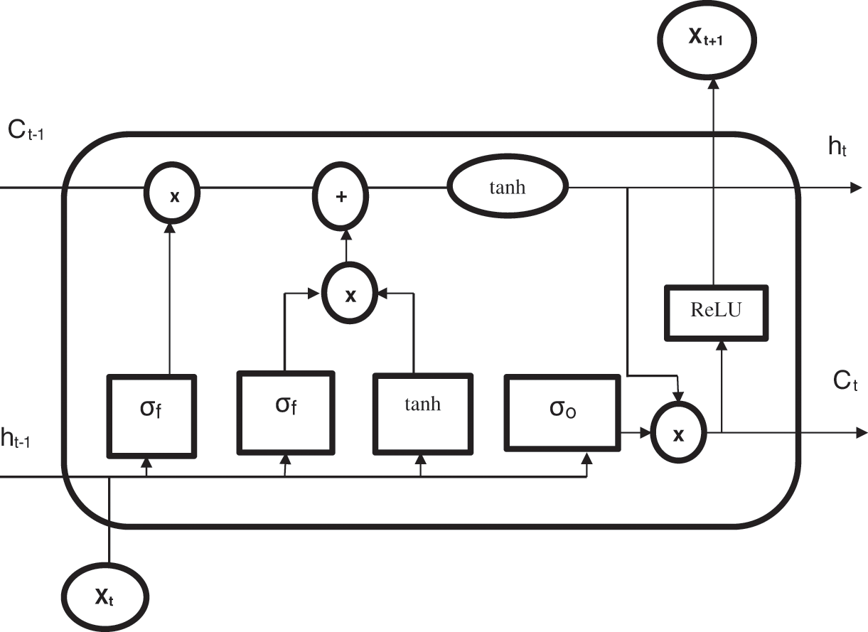
Figure 1: LSTM model

The mathematical derivation of forget state based on Xt (input) and ht (hidden layer activation functions) is expressed as follow,

Ft=σ(Wf[ht−1,xt]+bf (1)

whereσ → Sigmoid activation function,W → weight matricesb → threshold bias

σ(X)=11−e−x (2)

The Input Gate and output gates are activated to obtain a hidden cell state Ct. The hidden cell state is used to move the information into a new hidden cell state. Both the gates are performed by using a sigmoid (σ) and hyperbolic tangent function (tanh) activation function. Thus, the input gate (it) and an output gate with a new hidden cell state (ot) that is expressed in the following.

it=σ(wi[ht−1,xt]+bi (3)

ot=tanh⁡wo[ht−1,xt]+bo (4)

tanh(X)=ex′−e−x′ex′+e−x′,between −1 to 1 (5)

Objective Function

The objective function is defined by fine-tuning the weights and threshold bias of the LSTM hyperparameter. The fine-tuning is done by using the JellyFish search optimization which is obtained an optimal result. Based on this function, the approximate computing multiplier is trained by optimised LSTM to provide a pre-defined library function. This predefined library can be achieved an error rate reduction and high computational speed in approximate computing. Thus, the Mean Square Errors (MSE) can be formulated in terms of desired output of the approximate multiplier (Di) and a predicted output of Approximate multiplier (Pi) in below.

MSE=minimum(∑i=1N⁡(Di−Pi)2N) (6)

Based on the MSE value, the fine-tuning is performed by the novel jelly optimised LSTM algorithm in terms of weight and biases respectively.

4  Proposed Methodology

In this section, the proposed approximate multiplier based DL based library generation. This proposed approximate multiplier is aimed to reduce the power and area with improved error rate performance. The overall architecture of proposed approximate computing is shown in Fig. 2. The proposed Approximate Computing architecture comprises an input module, Approximate multiplier, Novel Jelly optimised LSTM model, Optimised Pre-trained Library and output module.

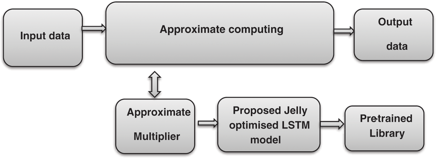
Figure 2: Novel approximate computing

From Fig. 2, the input module is used to fetch the data for computing that is sent to perform an approximate multiplier. The Approximate multiplier has two main processes namely Jelly optimised LSTM and pre-trained library. Initially, to provide an optimal solution with higher accuracy, the Jelly optimised LSTM is performed. This model has applied all the functional possibilities of an approximate multiplier. Then all these optimised values are stored in a library. The optimised pre-trained library is the memory block that is stored a maximum amount of data after jelly optimised LSTM is performed. Based on the input data, the approximate multiplier provides a corresponding output value to the output module. Finally, the output of the approximate computing is obtained with a minimum error rate, low power dissipation and high accuracy.

Therefore, the proposed Approximate computing has resulted in higher merits based on the Novel Jelly Optimised LSTM model (discussed below)

Proposed Novel Jelly Optimised LSTM

The Novel Jelly Optimised LSTM is proposed that is used to fine-tune the LSTM hyperparameters using JellyFish search optimization. The weight and threshold biases are the main hyperparameters of LSTM. These parameters are fine-tuned by JellyFish Search optimization to determine its objective function. This objective function is evaluated to provide the best optimal result. Later, the LSTM model is performed with a classification in approximate computing multiplier. Thus the optimal input awareness of approximate computing is achieved with greater accuracy by using a pre-trained Optimised LSTM. Therefore the JellyFish Search optimization is discussed in the following.

Jellyfish optimizer

Jellyfish is a very famous and well-known fish in an entire world which is lived from surface waters to the deep sea. It is structured as a soft body bell-shaped and long, harsh tentacles with various colours, shapes and sizes. The tentacles are used to attack and paralyze the prey by its venom. It has a special feature of allowing controlling its own movements. It is formed an umbrella structure to move forward by pushing water. Based on currents and tides, it is mostly drifting in the water. At a time of favourable condition, the jellyfish used to make a swarm to show its mass named as Jellyfish bloom. To form a jellyfish swarm, there are several parameters measured such as ocean currents, oxygen availability, available nutrients, predation, and temperature. The swarm formations are obtained with this parameter where ocean currents are the most significant factor for a swarm. Thus the Jellyfish Search algorithm is inspired by its searching characteristic and ocean movement. These fishes are made actions in three possible ways namely,

1.    It is lived either in an ocean current or towards the swarm; it has a “time control process that carried between these movement types.

2.    It is searched for food in the ocean and attracted to the location of maximum little fish prey or quantity is presented.

3.    Once the prey’s location is identified location and its objective function is evaluated.

The Jellyfish behaviour based on search food in the ocean is shown in Fig. 3.

Figure 3: Jellyfish behaviour in the ocean

Ocean current

The ocean current with numerous nutrients is attracted by jellyfish. The ocean current direction (trend) is expressed in Eq. (1).

trend→=X∗−β∗random(0,1)∗μ, (7)

where X∗→ current best position of jellyfish which is the mean value of every jellyfish location; β > 0 represents a coefficient of distribution towards trend length.

The position update of jellyfish is formulated in the following.

Xi(t+1)=Xi(t)+randon(0.1)∗trend→ (8)

Jellyfish swarm

A swarm is the collection of jellyfish in large quantities. It is moved in its original position known as passive motion, type A or a new position known as active motion, type B.

Thus, the Type A motion is expressed by updating its own position by using the following equation

Xi(t+1)=Xi(t)+γ∗randon(0.1)∗(UB−LB) (9)

where, UB → upper bound of search space, LB → lower bound of search space and γ → motion coefficient.

Thus the coefficient with the motion’s length is updated and considered as γ = 0.1

In Eq. (9), the type B movement is simulated. The jellyfish (j) is selected randomly to evaluate the movement direction. The jellyfish vector is chosen with an interest (i) to the selected jellyfish (j). If the preys are predicted at the location of chosen jellyfish (j) exceeds that jellyfish position of interest (i), then again moves to the first. When the prey is available for the selected jellyfish (j) is minimum than the jellyfish position of interest (i), then it will move away directly from the location Therefore every jellyfish is moved to determine better positions for prey by updated jellyfish position.

step→simulatedrandom(0,1)Dir→ (10)

Dir→={Xj(t)−Xi(t)iff(Xi)≥f(Xj)Xj(t)−Xj(t)iff(Xi)≥f(Xj) (11)

Xi(t+1)=−Xi(t)+step→ (12)

where f represents an objective function of position X

To evaluate the motion types over time, a time control mechanism is presented. This control mechanism controlled an overall swarm type A and type B motions and also a jellyfish movement toward an ocean current. Thus the time control mechanism is explained in the following.

Time control mechanism

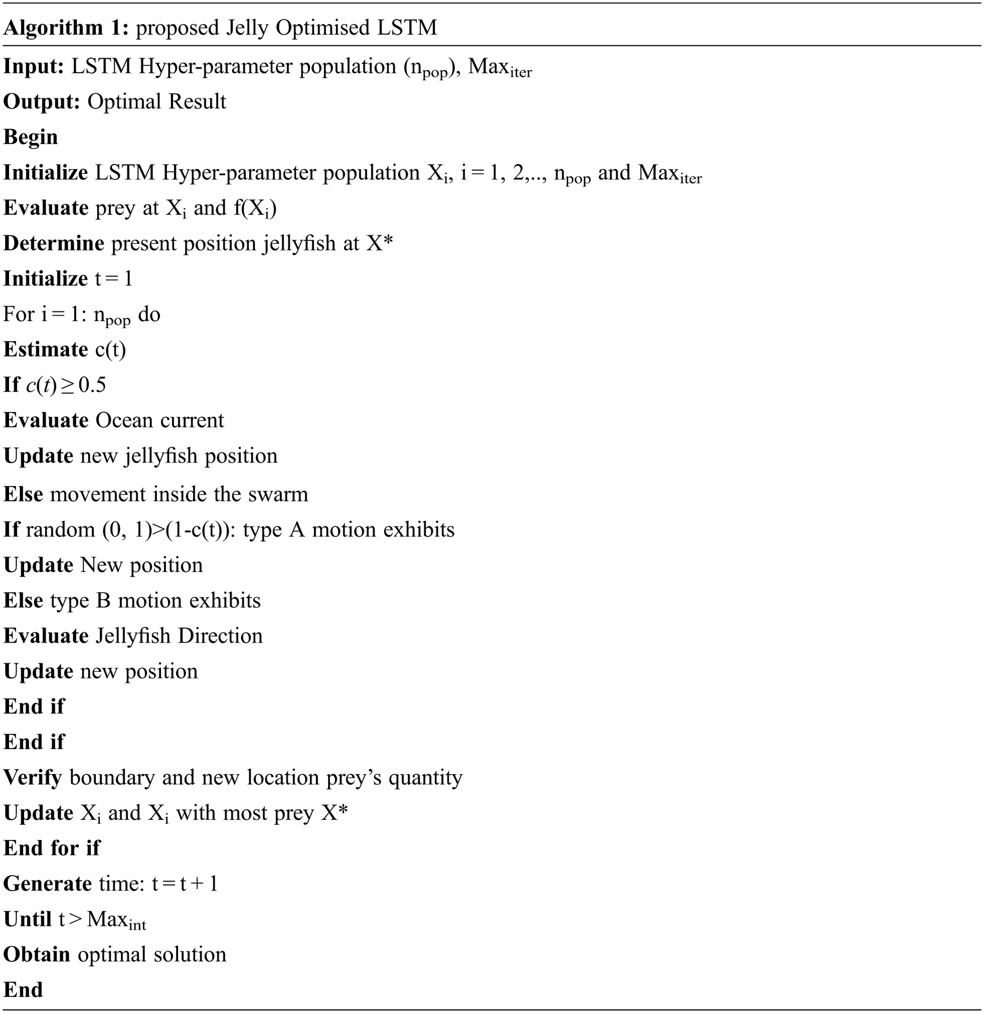
In this mechanism, the Jellyfish are often attracted to an ocean current because of its numerous nutritious plants. Frequently the temperature, wind and other atmospheric changes are carried in an ocean current. Then the jellyfish swarm migrated to another ocean current and form a new swarm in a new ocean current. The Jellyfish can be moved inside a swarm among type A and type B motion. Initially type A is selected for many overtimes, then type B is preferred gradually. To control the jellyfish movement between ocean current and between swarm, the Time control mechanism c(t) is expressed below.

c(t)=|1−1Maxiter∗(2∗random(0,1)−1)| (13)

where t represents a number of iterations in a specified time and Maxiter represents a maximum number of iterations. Therefore, jellyfish Search Optimization is discussed in algorithm 1.

Approximate multiplier design

The proposed jelly optimized LSTM model is trained with all possible combinations of multiplier inputs by varying truncation levels. The pretrained clusters are formed by the LSTM model to design an approximate multiplier with an optimal error rate. The knowledge about error rate and power consumption leads to improving the approximate performance of the proposed multiplier.

5  Performance Evaluation

The proposed multiplier is coded in Verilog and simulated using a synopsis compiler. The proposed multiplier compared with other conventional approximate multipliers like Under Designed Multiplier (UDM) [14] , Partial product perforation (PPP) [15], Static Segment Multiplier (SSM) [16] , Approximate compressor-based multiplier (ACM) [17] and Machine Learning based Approximate Multiplier(MLAM) in terms of area, delay, power mean relative error (MRE) and normalized error distance (NRE). In image processing applications, a geometric mean filter (GMF) is used to the smoothen image by removing unwanted noise. It performs geometric mean operations of pixels to enhance the image visual effects. The output image after performing GMF is given by

GMF(x,y)=[∏I(i;j)]1/mn (14)

where I denote the original image. Each pixel of the GMF processed image at point (x, y) is specified by the product of the pixels within the geometric mean mask raised to the power of 1/mn. To evaluate the efficiency of the proposed DL based multiplier, two 8-bits per pixel greyscale images with Gaussian noise are considered. The noisy images are filtered by applying a 3*3 mean filter with neighbouring pixels centred around them. The workflow of the proposed Peak signal-to-noise ratio (PSNR) and energy requirement is shown in Fig. 4. The performance of the proposed multiplier is given in Tab. 1. PSNR is the proportion among the extreme possible power of an image and the power of corrupting noise that disturbs the quality of its illustration. To calculate the PSNR, it is required to correlate that image to an ideal original image with the maximum possible power.

Figure 4: Proposed image processing performance analysis

In the proposed DL multiplier model, the approximated library is generated for all combinations of inputs. The truncation level of outputs with the corresponding area, energy, and error metrics are trained to the model to identify the best truncation bits and error compensation values. For 8-bit multiplier, 216 combinations of inputs and error metric for various truncation and error compensation values trained to LSTM model for selection best multiplication with the awareness of inputs.

Compared to other approximate multipliers, the proposed DL multiplier outperforms in terms of area, power and delay. Tab. 2 gives an error metric comparison of a proposed multiplier. From the results observed that the lower values of MRE and NRE prove the better suitability of the proposed multiplier in high power savings with more error tolerance applications.

The PSNR and energy savings of noisy images with resultant geometric mean filtered images are given in Tab. 3. The energy requirement of ML and DL based approximate multiplier is 1.90 and 1.34 μJ respectively. PSNR outputs of ML and DL based approximate multiplier is 71.5 and 74.9 respectively.

6  Conclusion

Approximate computing or inexact computing is used in numerous applications. Several researchers are worked on the low power approximate multiplier to improve the performance of Approximate computing. In this work, the novel Jelly optimised LSTM techniques are presented for an approximate multiplier. The approximate multiplier is obtained a highly optimised pre-trained input data using Jelly optimised LSTM techniques. The proposed technique is performed by fine-tuning the LSTM hyperparameters using jellyfish search optimisation. Based on the input aware knowledge of the pre-trained library, the performance of Approximate computing is increased. Therefore, the proposed Approximate computing is obtained a low power and minimum error rate than the previous model. Further, the performance of the proposed work is evaluated in terms of area, power and accuracy with the previous techniques. As a result, the proposed work is achieved a higher performance in all metrics than existing.

Funding Statement: The authors received no specific funding for this study.

Conflicts of Interest: The authors declare that they have no conflicts of interest to report regarding the present study.

This work is licensed under a Creative Commons Attribution 4.0 International License, which permits unrestricted use, distribution, and reproduction in any medium, provided the original work is properly cited.