DOI:10.32604/csse.2023.024633
| Computer Systems Science & Engineering DOI:10.32604/csse.2023.024633 | |
| Article |
Data-Driven Load Forecasting Using Machine Learning and Meteorological Data
Department of Computer Science, College of Computer, Qassim University, Buraydah, Saudi Arabia
*Corresponding Author: Ali Mustafa Qamar. Email: al.khan@qu.edu.sa
Received: 25 October 2021; Accepted: 10 December 2021
Abstract: Electrical load forecasting is very crucial for electrical power systems’ planning and operation. Both electrical buildings’ load demand and meteorological datasets may contain hidden patterns that are required to be investigated and studied to show their potential impact on load forecasting. The meteorological data are analyzed in this study through different data mining techniques aiming to predict the electrical load demand of a factory located in Riyadh, Saudi Arabia. The factory load and meteorological data used in this study are recorded hourly between 2016 and 2017. These data are provided by King Abdullah City for Atomic and Renewable Energy and Saudi Electricity Company at a site located in Riyadh. After applying the data pre-processing techniques to prepare the data, different machine learning algorithms, namely Artificial Neural Network and Support Vector Regression (SVR), are applied and compared to predict the factory load. In addition, for the sake of selecting the optimal set of features, 13 different combinations of features are investigated in this study. The outcomes of this study emphasize selecting the optimal set of features as more features may add complexity to the learning process. Finally, the SVR algorithm with six features provides the most accurate prediction values to predict the factory load.
Keywords: Electricity load forecasting; meteorological data; machine learning; feature selection; modeling real-world problems; predictive analytics
Global warming and energy security are the most critical problems that face the world today [1]. In addition, energy efficiency is one of the most significant issues that many countries attempt to improve. Renewable energy resources, such as Photovoltaic systems and Wind, have proven their efficacy to minimize non-friendly emissions [2]. Furthermore, such resources lead to an increase in energy efficiency as part of the electricity consumption is supplied from these sources. Nevertheless, the complexity accompanied by the electricity consumption is somewhat still a challenge due to the variation in the electricity demand, which causes an acute imbalance between the electricity supply and demand [3]. Therefore, predicting the actual behavior of the load is crucial for reliable operations of the electrical network.
In electrical power systems, machine learning algorithms have been used to tackle a variety of forecasting applications, including load forecast, market price forecast, Photovoltaics power forecast, and fault detection forecast [4]. Among these applications, load forecasting plays a significant role in different electrical power system applications, including the development of power systems, promoting the integration of solar and wind energy, and supporting demand-side management [5].
In Saudi Arabia, for example, the electricity consumption of residential, governmental, commercial, educational, industrial, and mosque buildings has increased with the steady growth in the population. According to the Saudi Energy Efficiency Center, 47% of Saudi Arabia's primary energy is consumed by the industry sector [6]. This makes forecasting the industrial load building important not only to capture the stochastic behavior of the load but also to facilitate embracing the ongoing renewable energy projects to supply to such types of buildings. Hence, the main goal of this research is to forecast an industrial load represented by a factory load.
To forecast the electricity load, three main steps need to be fulfilled to ensure accurate forecasting outcomes [7]. First, there are pre-forecasting steps that should be accomplished and satisfied to make the prediction results accurate. To create a load forecasting model, such models require input dataset to build them. Second, to forecast the electrical load of a certain type of building requires coming up with a forecasting model that mainly depends on different types of features. The meteorological features have shown a significant relationship with the electrical load consumption [8]. According to the recent systematic review conducted in [1], meteorological data are used frequently as learning inputs for building energy performance forecasts to train machine learning algorithms. These variables are highly dependent on the geographic location and the type of weather conditions at the site. In addition, the behavior of load tends to be repeated frequently, which shows that the historical load data (past electricity load usage) could have an impact on the load forecast. Finally, the machine learning algorithm that is responsible to predict the future load should be selected in a way that provides the most accurate prediction results. All these steps are applied and investigated in this study.
Different load types have been forecasted in the literature, including commercial, residential, industrial, educational buildings, and distribution feeders. In [9], a day-ahead residential load is predicted for a granularity of 15, 60, and 120 mins. Weather data, historical load data, and calendar effect were considered inputs to the forecasting methods. In this study, multiple linear regression (MLT), regression trees (RT), artificial neural network (ANN), and support vector regression (SVR) are employed. This work concludes that RT generally has the best performance, while SVR is the best in estimating the household load for the next 24 h. The root mean squared error (RMSE) value using RT is the lowest with 0.516 kWh, followed by SVR and ANN with 0.53 and 0.531 kW, respectively.
The study in [10] uses a neural network algorithm to predict the short-term electrical load in Nepool city from 2004 to 2008. In the training phase, the data from 2004 to 2007 are used to train the ANN, and the 2008 data were used for testing. To evaluate the load forecasting model, the mean absolute error (MAE) and mean absolute percentage error (MAPE) are used. The study found that MAPE gave a rate of 1.38% on weekdays, and 1.39% on weekly holidays. The results state that the forecasting model gives slightly lower error rates on weekdays as compared to the weekends. The study also found that the weather factor affects the prediction process, such as temperature and wind speed.
The authors in [11] predict the electrical load for a whole week from July 16 to July 22, where they collected data from the local Electrical Distribution Company from March 2010 to July 2010. Their study uses SVR and ANN as prediction algorithms. The study found that the SVR model gave the lowest MAPE with a value of 1.6%, while the ANN model has a MAPE value of 2.18%.
The electrical load is predicted for the next day in urban areas using weather data in [12]. ANN and the Bagged Regression Trees are used to forecast the electrical load. The two algorithms are compared to verify the accuracy of the prediction. The comparison is evaluated based on the MAE, MAPE, and Daily Peak MAPE. The study concludes that Bagged Regression Trees provide more accurate prediction results than ANN. The results show that the Bagged Regression Trees give a MAPE of 1.54%, MAE of 136.39 MW, and Daily Peak MAPE of 1.67%. On the other hand, the ANN algorithm’s error values were found to be MAPE = 1.90%, MAE = 167.91 MW, and Daily Peak MAPE = 2.08%. In addition, the short-term electrical load (for one day) in Jinan during 2016 was predicted using the LS-SVM regression model in [13]. The load is trained based on data from June and July, while the maximum temperature and average temperature are used as inputs. The proposed forecasting model gives a great prediction accuracy when using the maximum temperature and average temperature. The study also finds that the accuracy of the daily load depends on the accuracy of the prediction of the daily maximum and minimum load and, a high temperature increases the load.
The researchers in [14] present the prediction of the daily electrical load in Thailand from January 1, 2013, to December 31, 2014. ANN is used to predict the daily load with the temperature factor, where the electrical load data were tested for 30 minutes. The study results reveal that the prediction algorithm gives a high prediction accuracy, and the prediction is more accurate when the temperature is included as one of the input factors. Furthermore, the researchers in [15] conduct a comparison between ARIMA and SVM algorithms to predict the daily electrical load (short term) from March 18 to May 18 for 28 consumers. The comparison is made using MAPE and MSE, and the results indicate that the SVM algorithm provides better prediction accuracy than ARIMA.
In [16], the authors build a short-term electrical load forecasting model using the random forest algorithm. The forecasted values are then compared to the measured electrical load for a given region from January 1. The results show that the random forest gives a high degree of prediction where results for MAPE = 1% and R2 is greater than 0.99. The study in [17] presents an analysis of electrical load data for 365 days of 2019 in Macedonia using ANN. For model evaluation, the MAE (%), MSE (MW2), and RMSE (MW) error metrics are used. The study concluded that the algorithm provides a great prediction accuracy, and the percentages were as follows: MAE = 3.04%, MSE = 1397 MW, and RMSE = 37.38 MW.
Furthermore, the researchers in [18] predict the electrical load in Qingdao, China using ANN. The datasets are collected for the electrical load data from January 1, 2016, to December 31, 2018. The study finds that the evidence of electrical load varies between days, pointing out that the electrical load decreases during the days of national festivals and long holidays. Also, the study finds that on hot summer days, the electrical load increases as compared to other days when the weather is mild. This implies that the past load observations may impact forecasting the future load.
From the aforementioned discussion, the meteorological and historical load data are the two types of features that may have an impact on forecasting the electrical load. In addition, the machine learning algorithms prove their efficacy in a variety of forecasting applications. Hence, the main contributions of this study are summarized as follows:
• To develop a data-driven forecasting model of the electrical load of a factory located in Riyadh, Saudi Arabia. A short-term (24 h ahead with one-hour time step) load forecast is accomplished in this study utilizing different machine learning algorithms, namely ANN and SVR based on Radial Basis, Polynomial, and Linear Kernel functions.
• To study the impact of historical load and meteorological data on load forecast. The weather data considered in this study are Air temperature, Cloud Capacity, Global Horizontal Irradiance, Relative Humidity, Barometric Pressure, Wind Direction, and Wind Speed. The primary goal of considering such variables is to investigate their influence on the electrical load, which may help the decision-makers solve problems in an electrical load before they occur.
• To compare the performance of ANN and SVR in forecasting the electrical load of the factory.
• To build an electrical load forecasting framework that may help other researchers, who are interested in load forecast, to start with.
3 Framework of the Forecasting Models
This study uses different feature schemes to evaluate the impact of the meteorological variables on load forecast. For that reason, all features schemes are compared with other selected features schemes to obtain the optimal set of features that led to the most accurate prediction results. The selection of these features is based on the Pearson autocorrelation values. Finally, the prediction results of the load of the factory are interpreted, compared, and discussed. A total of 52 forecasting models are created for the goal of forecasting the factory load. The forecasting objective and the forecasting models generated in this study are as follows:
Forecasting Objective: A forecasting model for the factory load
• ANN with 13 different sets of features (Fi) (ANN–Fi).
• SVR based on the Radial Basis function with 13 different sets of features (Fi) (SVR–RB–Fi ).
• SVR based on a Polynomial function with 13 sets of features (Fi) (SVR–Poly–Fi).
• SVR based on a Linear function with 13 sets of features (Fi) (SVR–Linear–Fi).
where (Fi) is the set of features and i is the number of features in that set.This study uses MATLAB R2021 and the fitrsvm function to implement SVR-based kernel functions. On the other hand, for the ANN network, the backpropagation network (BPNN) is selected, and the ANN Tool in MATLAB is used to implement the network. Fig. 1 shows the main framework used to construct this study and to predict the load of the factory.
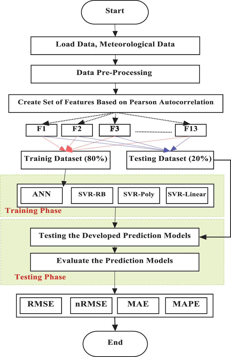
Figure 1: Framework of the factory load forecast
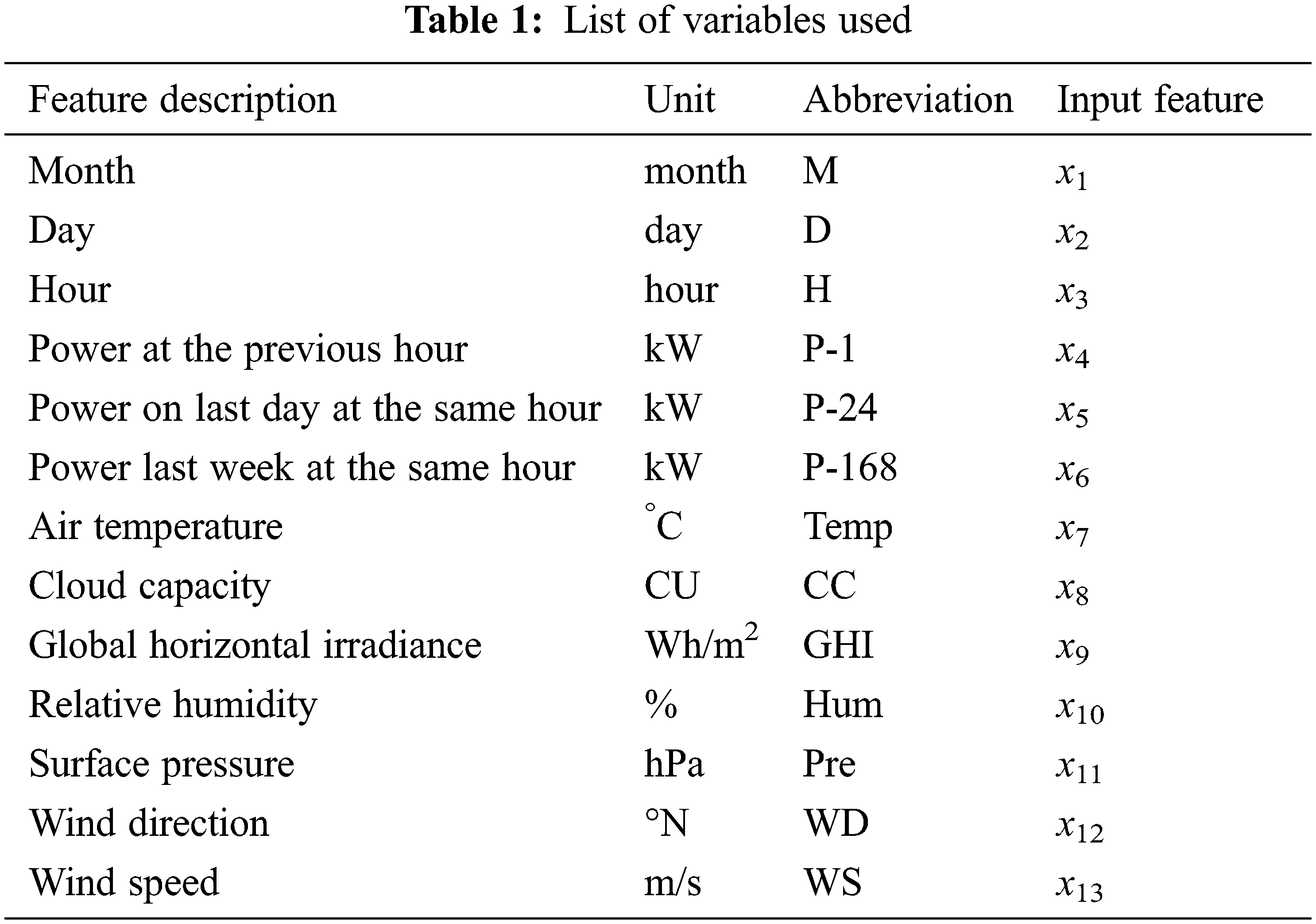
In the first step of the framework, the data are collected and organized. The data include the factory load and the meteorological datasets. Similarly, in the next step, the data preprocessing techniques are applied to prepare the data. These include data collection, data cleaning, data monitoring, and data normalization processes. The data pre-processing techniques are discussed in detail in Section 4. Moreover, in the third step, different sets of features (13), as shown in Tab. 1, are constructed based on the Pearson autocorrelation values.
In the fourth step, the data are divided into two sets: training and testing. The training data are utilized to train the machine learning algorithms and the test set is used to examine the accuracy of the prediction models. Later, in the fifth step, SVR and ANN are applied to build the forecasting models for each forecasting objective using the formulated set of feature schemes. All the training models are exposed to the same set of data. Lastly, in the sixth step, the test dataset is used to evaluate each of the prediction models, and the best forecasting model is then selected. The evaluation is done based on the following evaluation metrics: RMSE, normalized Root Mean Square (nRMSE), MAE, and MAPE.
4 Data Preprocessing Techniques
Machine learning algorithms need data pre-processing and cleaning stages to prepare the data for the learning algorithm. For instance, the data used in this research work are obtained from different sources. Therefore, the data are required to be organized to create the set of data that are fed to the learning algorithms. In the field of data analysis, three main observations need to be acquired: data, information, and knowledge [19,20]. In this sense, the data can be transformed and integrated into information that can later be visualized and interpreted to obtain the desired knowledge. This knowledge can later help in taking the necessary decision. Fig. 2 shows the big data transformation and analysis process. These processes are followed and applied in this study.
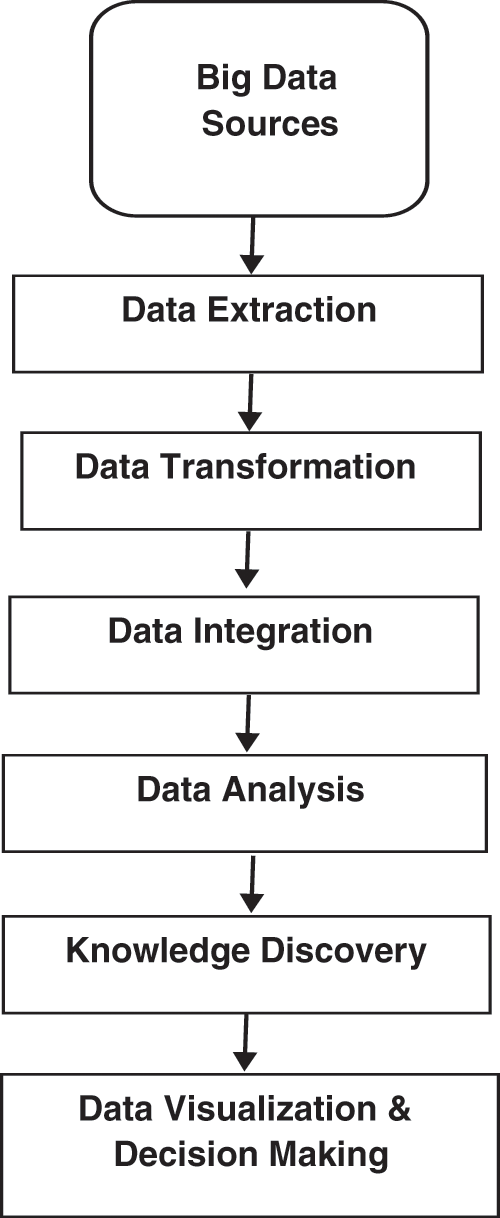
Figure 2: Big data analysis process [19]
The data to be analyzed can come from different data providers. This can add difficulty to the data and impact their reliability if they come from unreliable sources. In addition, these data are subjected to be imprecise which adds difficulties to deal with. Therefore, importing and collecting data from reliable sources is very significant that results in accurate data analysis [20]. In this study, the data are collected from different reliable sources. The data are obtained from SEC and King Abdullah City for Atomic and Renewable Energy (K.A.CARE). The data from SEC are real-world data gathered in real-time from the electrical meter of a factory, while the KACARE's data are obtained from different data sensors located at the same site as that of the factory.
After getting the data from reliable data sources, the data are required to be extracted. Some of the data providers make the data publicly available. In other words, the data can be downloaded freely. On the other hand, prior permission is required by some data resources due to their confidentiality. Other providers are offering the data with fees, which vary depending on the data amount. In this study, the data are collected from SEC and K.A.CARE with prior permission to use these data.
In this stage, the data are converted to a consistent form. That is, they are transformed from the form of the extraction to the structure of data to be utilized [21]. All the data have the same format, which helps in dealing with this data. In this study, all the data are transformed to be on one workstation.
Data integration is a crucial step in data processing. The data need to be integrated uniquely and uniformly [22]. The data used in this study are organized consistently to become analyzable by machine learning algorithms. As mentioned previously, the data used in this work are obtained from different sources. Therefore, the data are merged based on the timestamp. Furthermore, the time is obtained in this form: “YYYY-MM-DD-HH”. For data preparation, the time is separated into different variables.
Data analysis is the step when we go deep into the data. In this step, many hidden features in the dataset will be revealed that helps in forecasting the future values of the factory load [19]. Moreover, the data analysis allows us in exploring the hidden patterns existing in the extracted data. One of the key elements of data analysis is statistical features [23]. The statistical features, such as average, variance, minimum value, maximum value, and correlation values, are important in evaluating the data. The following are the four key steps associated with the data analysis process: input data, data collection, data processing (organize the data into columns and rows), and data cleaning.
Data are subjected to be missing or imprecise. The data used to forecast the factory load are usually based on the past readings of different variables. Using faulty input data will impact the accuracy of the forecasting algorithms [24]. Hence, cleaning the data and detecting the unwanted data is a very crucial step in data pre-processing. Dealing with a huge amount of data makes manual cleaning of data a very sophisticated process.
With data cleaning, we can attain different objectives in the interest of building a precise load forecasting model. Some of the benefits of applying data cleaning process are as follows [25]:
• In data extraction, a variety of observations is expected to be obtained. These observations may be redundant or irrelevant to the problem at hand. The data cleaning helps in removing such observations to create a set of data that are manageable and meaningful.
• As mentioned previously, the data are transformed into one structure which could create structural errors. Data cleaning can help in capturing such errors that could be fixed in the data transformation step.
Both electrical buildings’ load and meteorological datasets are forms of data that may contain hidden patterns that are required to be investigated and studied. In this study, the meteorological data are analyzed through different data mining techniques aiming to predict the electrical load of a factory. The factory selected in this study is located in Riyadh, Saudi Arabia. Therefore, the meteorological data are gathered from a station located in Riyadh, and these data are recorded hourly from 2016 to 2017 by K.A.CARE. On the other hand, the factory load is recorded also hourly from 2016 to 2017 and is collected from the Saudi Electricity Company (SEC). The data of one year is sufficient since it covers all seasons (fall, winter, spring, and summer) and the electrical load variation due to the seasonality will be captured by machine learning algorithms. Fig. 3 shows the solar map of Saudi Arabia.

Figure 3: Solar map of Saudi Arabia [26]
Obtaining the correlation values is a critical step for comprehending and visualizing the datasets. The Pearson correlation coefficient is used to determine the degree of correlation between two variables. Pearson correlation is represented in Eq. (1), where cov is the covariance, σWeather and σLoad are the standard deviations of weather variables xWeather and the load values xload, respectively.
Fig. 4 displays the correlation values of each of the considered features with the load of the factory.
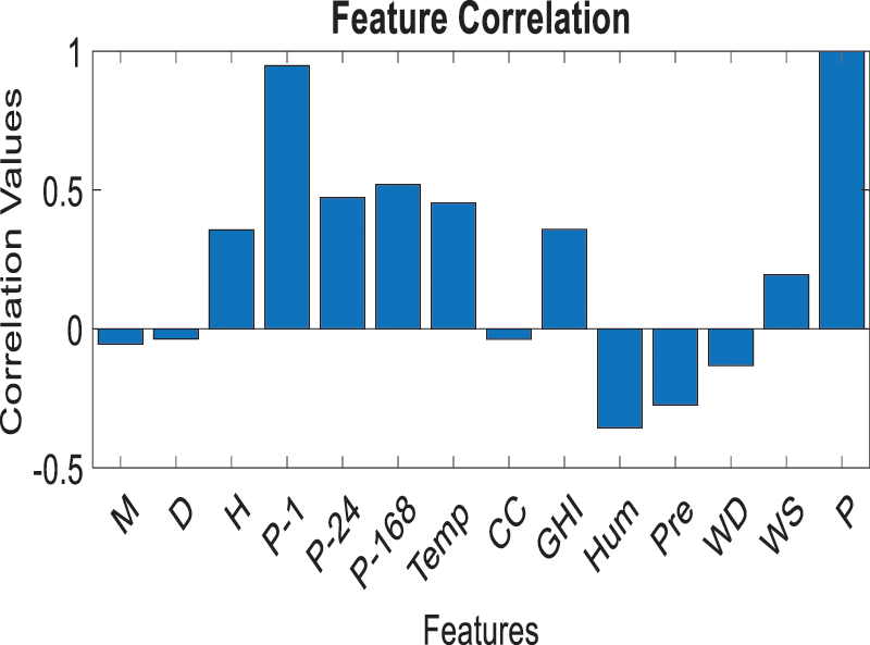
Figure 4: Correlation values of the variables with the factory load
As mentioned previously, some of these variables have no impact on the forecasting outcomes and may add complexity to the forecasting process. From this, a total of 13 sets of features are formulated that contain different features. Tab. 2 lists the different sets of features for which the goal is to select the best set of features that provide the most accurate prediction values.

In this study, 13 sets of features are created to predict the factory load. These features are formulated based on their correlation values with the factory load, as presented in Fig. 4. For instance, the feature set (F1) contains one feature that has the highest correlation value. This feature is (P–1), which is the power at the previous hour in kW. Similarly, the F2 contains F1 and has the second-highest correlation value, which is the power last week at the same hour in kW (P–168). A similar analogy exists with the remaining set of features. The variables used in this study to forecast the factory load have different numerical scales. For example, the variable D, which is the Day, has values between 1 and 31, while the variable GHI, which is the Global Horizontal Irradiance, has values from 0 to 1038 Wh/m2. This variation of numerical values among the input variables affects negatively the learning process. That is, the machine learning algorithms will add higher weight to the variables with greater numerical values, which will eventually impact the prediction outcomes. Therefore, and to avoid this obstacle, all the prediction variables need to be normalized to be between a specific range. Through using data normalization or what is called dimensionality reduction, the data have the same weight without losing information in the input data. In this study, the input data listed in Tab. 1 are normalized between 0 and 1 using Eq. (2).
where xi is the actual data value; xin is the normalized value, while xmax and xmin are the maximum and minimum values corresponding to the actual dataset, respectively.
8.1 Artificial Neural Networks
ANN is an information computing system that mimics the approach that the human brain analyzes the information. ANN is created similar to the human brain where a huge number of neuron nodes are interconnected to tackle problems that represent the uniqueness of this network.
In this research, the number of hidden layers is selected and identified based on trial and error until we attain the most suitable number of hidden layers that provide an ANN model with high accuracy. The optimal number of hidden layers is obtained when the nodes are equal to the number of input features. For example, three nodes are used with F3, while seven nodes with F7. The model output, therefore, can be calculated using Eq. (3) [27]:
where m is the number of nodes at the input layer, n is the number of nodes in the hidden layer, f is a sigmoid transfer function, which will be the logistic function in this research. Similarly,
Support vector machine (SVM) is a supervised learning approach utilized for classification, regression problems, or outliers’ detection. When two classes cannot be separated, a kernel function is employed to map the input space to a higher-dimensional space. In that new space, the input space may be separated linearly [10]. To conduct the separation, there are three known kernel functions which are: radial basis (RB), polynomial (Poly), and linear functions [28]. Hence, SVR inherently employs some of the SVM properties. Unlike SVM, SVR conducts the classification based on the regression process error measures based on a predefined threshold, as shown in Fig. 5 [29].
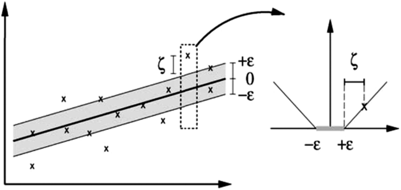
Figure 5: The boundary margin and loss setting for a linear SVR [29]
In this study, the performance of the three kernel functions to predict the factory load is compared with ANN. The leading optimization can be formulated in Eq. (4), and the kernels that are used in this work with SVR are provided in Eqs. (5)–(7) [13]. The SVR requires to solve the following optimization problem:
where C > 0 is a constant that identifies the trade-off between the flatness of f and assesses the tolerated amount of deviation to values larger than ε, see Fig. 5. As mentioned earlier, our input space is represented by the input features, or the training dataset is transferred into a new space with high dimensions while using the function ϕ. This is known as the kernel trick (xi, xj) = ϕ(xi)T(xj). The kernel functions used in our models can be written as:
where γ (Gamma) and d are the kernel parameters. In this study, the parameters associated with RB and Poly kernel functions are set to the default values.
To evaluate the models that are built in this study, different statistical indicators are used. These include Root Mean Square Error (RMSE), normalized Root Mean Square (nRMSE), Mean Absolute Error (MAE), and Mean Absolute Percentage Error (MAPE). These metrics can be expressed by Eqs. (8)–(11), respectively [30]:
where n is the length of the testing set, yi is the measured or observed electrical load values to estimate,
In this subsection, the results of forecasting the factory load are presented. This includes the results of the best forecasting algorithm and the best set of features that result in the best forecasting values for the considered load. Fig. 6 displays the RMSE and the MAE in kW for all the forecasting models built to forecast the factory load.

Figure 6: RMSE and the MAE in kW for all the forecasting models
In addition, Tab. 3 lists the statistical results of all the forecasting models with a set of features considered in this study (F6 and F10).

10.2 Best Forecasting Algorithms to Forecast Factory Load
As mentioned earlier, four forecasting algorithms are built to forecast the factory load. According to Fig. 6 and Tab. 3, the SVR-RB models have the best forecasting results. The ANN can be considered the second-best prediction algorithm, while the SVR-Poly and SVR-Linear are the third and the fourth-best forecasting algorithms, respectively. Taking, for example, the results with the feature set F10, the SVR-RB forecasting model has an RMSE value of 11.66 kW and an MAE of 8.25 kW, while the ANN model has an RMSE value of 13.39 kW and an MAE value of 9.69 kW. Similarly, with all other forecasting models, the SVR-RB leads to the best forecasting results followed by ANN and SVR-Poly models. The SVR-Linear model can be considered the worst as it leads to the largest statistical errors.
10.3 The Best Set of Features to Forecast Factory Load
According to Fig. 6 and Tab. 3, set F6 led to the best forecasting results as compared to the other sets. As listed in Tab. 2, this set includes power at the previous hour (P–1), power last week at the same hour (P–168), power on the last day at the same hour (P–24), Temperature (Temp), Hour (H), and GHI. Therefore, to predict the factory load, 6 out of 13 features are sufficient to predict the load. On the actual operation of the factory, these time, historical load readings, and the outdoor heating variables have a major impact on electrical consumption. The load of the factory is frequently repeated, hourly, and weekly, as the factories usually follow specific production lines, which justify the time and historical reading variables. Also, the efficiency of the factory's equipment is highly dependent on the outdoor temperature and solar radiation. Therefore, more features or attributes do not always bring about good prediction results, and selecting the appropriate features is very crucial, which is accomplished in this study.
Figs. 7 and 8 show the regression plots of the forecasted values with a set of features F1, F6, F10, and F13, respectively, when they are plotted against the measured factory load readings using the SVR-RB forecasting algorithm. It can be shown that SVR-RB with F6 has the best regression plot as the data concentrate around the regression line.

Figure 7: Regression plot of the measured vs. forecasted load with F1 and F6

Figure 8: Regression plot of the measured vs. forecasted load with F10 and F13
The best forecasting model to predict the factory load is by using the SVR-RB algorithm with the feature set F6 (SVR-RB-F6). Tab. 3 shows that the statistical error with this model is the minimum with RMSE of 11.63 kW, nRMSE of 3.21%, MAE of 8.21 kW, and MAPE of 6.02%. For further visualization, Fig. 9 shows the performance of the four forecasting algorithms to forecast the factory load with the feature set F6 on three different test days. It can be noticed that SVR-RB has the best performance as it can track the measured factory reading compared to other forecasting models.

Figure 9: The performance of the four forecasting algorithms to forecast the factory load with the feature set F6 on three different test days
In this study, a factory load located in Riyadh, Saudi Arabia, is forecasted using four machine learning algorithms, namely Artificial Neural Network, Support Vector Regression based on Radial Basis function (SVR-RB), Support Vector Regression based on Polynomial function, and Support Vector Regression based on Linear function. To predict the factory load, 13 independent variables are used. However, and from the fact that more features do not always provide accurate forecasting outcomes, 13 sets of features are formulated to identify the set that provides the most accurate forecasting values. The selection of these sets was conducted based on the features correlation values with the actual reading of the factory load. To evaluate the performance of the built forecasting models, some statistical indicators are used, namely Root Mean Square Error (RMSE), normalized Root Mean Square Error (nRMSE), Mean Absolute Error (MAE), and Mean Absolute Percentage Error (MAPE).
The results show that SVR-RB is the best forecasting algorithm to forecast the factory load. For the factory load, the SVR-RB with six features (SVR-RB-F6) resulted in the lowest statistical error with RMSE of 11.63 kW, nRMSE of 3.21%, MAE of 8.21 kW, and MAPE of 6.02%. The SVR-RB proves its ability to forecast the factory load with high accuracy results. Moreover, the selection of the best features is very important to create forecasting models that best predict the factory loads. Finally, in this study four machine learning algorithms are investigated. Other algorithms, such as random forest, decision trees, or deep learning algorithms, can be also investigated to forecast the load and their forecasting results can be compared with the results of this study.
Acknowledgement: The researchers would like to thank the Deanship of Scientific Research, Qassim University for funding the publication of this project.
Funding Statement: The researchers would like to thank the Deanship of Scientific Research, Qassim University for funding the publication of this project.
Conflicts of Interest: The authors declare that they have no conflicts of interest to report regarding the present study.
1. S. Fathi, R. Srinivasan, A. Fenner and S. Fathi, “Machine learning applications in urban building energy performance forecasting: A systematic review,” Renewable and Sustainable Energy Reviews, vol. 133, pp. 110287, 2020. [Google Scholar]
2. S. Karkour, Y. Ichisugi, A. Abeynayaka and N. Itsubo, “External-cost estimation of electricity generation in G20 countries: Case study using a global life-cycle impact-assessment method,” Sustainability, vol. 12, no. 5, pp. 2002, 2020. [Google Scholar]
3. G. Chitalia, M. Pipattanasomporn, V. Garg and S. Rahman, “Robust short-term electrical load forecasting framework for commercial buildings using deep recurrent neural networks,” Applied Energy, vol. 278, pp. 115410, 2020. [Google Scholar]
4. S. M. Miraftabzadeh, M. Longo, F. Foiadelli, M. Pasetti and R. Igual, “Advances in the application of machine learning techniques for power system analytics: A survey,” Energies, vol. 14, no. 16, pp. 4776, 2021. [Google Scholar]
5. L. Wen, K. Zhou and S. Yang, “Load demand forecasting of residential buildings using a deep learning model,” Electric Power Systems Research, vol. 179, pp. 106073, 2020. [Google Scholar]
6. A. Al Ghamdi, “Saudi Arabia energy report,” Discussion Papers ks--2020-dp25, King Abdullah Petroleum Studies and Research Center, 2020. [Google Scholar]
7. J. Grus, Data Science from Scratch: First Principles with Python, 1st ed., Sebastopol, CA, USA: O'Reilly Media, 2015. [Google Scholar]
8. C. -L. Hor, S. J. Watson and S. Majithia, “Analyzing the impact of weather variables on monthly electricity demand,” IEEE Transactions on Power Systems, vol. 20, no. 4, pp. 2078–2085, 2005. [Google Scholar]
9. P. Lusis, K. Rajab Khalilpour, L. Andrew and A. Liebman, “Short-term residential load forecasting: Impact of calendar effects and forecast granularity,” Applied Energy, vol. 205, pp. 654–669, 2017. [Google Scholar]
10. S. Singh, S. Hussain and M. A. Bazaz, “Short term load forecasting using artificial neural network,” in Proc. Fourth Int. Conf. on Image Information Processing, Shimla, India, pp. 1–5, 2017. [Google Scholar]
11. S. Fattaheian-Dehkordi, A. Fereidunian, H. Gholami-Dehkordi and H. Lesani, “Hour-ahead demand forecasting in smart grid using support vector regression (SVR),” International Transactions on Electrical Energy Systems, vol. 24, no. 12, pp. 1650–1663, 2014. [Google Scholar]
12. V. Dehalwar, A. Kalam, M. L. Kolhe and A. Zayegh, “Electricity load forecasting for urban area using weather forecast information,” in Proc. IEEE Int. Conf. on Power and Renewable Energy (ICPRE), Shanghai, China, pp. 355–359, 2016. [Google Scholar]
13. L. Hu, L. Zhang, T. Wang and K. Li, “Short-term load forecasting based on support vector regression considering cooling load in summer,” in Proc. Chinese Control and Decision Conf. (CCDC), Hefei, China, pp. 5495–5498, 2020. [Google Scholar]
14. M. H. M. R. S. Dilhani and C. Jeenanunta, “Daily electric load forecasting: Case of Thailand,” in Proc. 7th Int. Conf. of Information and Communication Technology for Embedded Systems (IC-ICTES), Bangkok, Thailand, pp. 25–29, 2016. [Google Scholar]
15. M. A. Al Amin and M. A. Hoque, “Comparison of ARIMA and SVM for short-term load forecasting,” in 9th Annual Information Technology, Electromechanical Engineering and Microelectronics Conf. (IEMECON), Jaipur, India, pp. 1–6, 2019. [Google Scholar]
16. H. Yiling and H. Shaofeng, “A Short-term load forecasting model based on improved random forest algorithm,” in Proc. 7th Int. Forum on Electrical Engineering and Automation, Hefei, China, pp. 928–931, 2020. [Google Scholar]
17. G. Veljanovski, M. Atanasovski, M. Kostov and P. Popovski, “Application of neural networks for short term load forecasting in power system of north Macedonia,” in Proc. 55th Int. Scientific Conf. on Information, Communication and Energy Systems and Technologies, Serbia, pp. 99–101, 2020. [Google Scholar]
18. H. Dong, Y. Gao, X. Meng and Y. Fang, “A multifactorial short-term load forecasting model combined with periodic and non-periodic features –A case study of Qingdao, China,” IEEE Access, vol. 8, pp. 67416–67425, 2020. [Google Scholar]
19. V. V. Kolisetty and D. S. Rajput, “A review on the significance of machine learning for data analysis in big data,” Jordanian Journal of Computers and Information Technology (JJCIT), vol. 6, no. 1, pp. 41–57, 2020. [Google Scholar]
20. Y. Roh, G. Heo and S. E. Whang, “A survey on data collection for machine learning: A big data-AI integration perspective,” IEEE Transactions on Knowledge and Data Engineering, vol. 33, no. 4, pp. 1328–1347, 2021. [Google Scholar]
21. B. Wujek, P. Hall and F. Güneş, “Best practices for machine learning applications,” SAS Institute Inc, pp. 1–23, 2016. [Google Scholar]
22. R. Ahmed, V. Sreeram, Y. Mishra and M. D. Arif, “A review and evaluation of the state-of-the-art in PV solar power forecasting: Techniques and optimization,” Renewable and Sustainable Energy Reviews, vol. 124, pp. 109792, 2020. [Google Scholar]
23. B. Sharma, “Processing of data and analysis,” Biostatistics and Epidemiology International Journal, vol. 1, no. 1, pp. 3–5, 2018. [Google Scholar]
24. G. Y. Lee, L. Alzamil, B. Doskenov and A. Termehchy, “A survey on data cleaning methods for improved machine learning model performance,” arXiv preprint, arXiv: 2109.07127, pp. 1–6, 2021. [Google Scholar]
25. “Guide to data cleaning: Definition, benefits, components, and how To clean your data.” [Online]. Available: https://www.tableau.com/learn/articles/what-is-data-cleaning. [Accessed: 14-Oct-2021]. [Google Scholar]
26. “Solar resource maps of Saudi Arabia and GIS data | Solargis.” [Online]. Available: https://solargis.com/maps-and-gis-data/download/saudi-arabia. [Accessed: 03-Oct-2020]. [Google Scholar]
27. A. Nespoli, E. Ogliari, S. Leva, A. M. Pavan, A. Mellit et al., “Day-ahead photovoltaic forecasting: A comparison of the most effective techniques,” Energies, vol. 12, no. 9, pp. 1621, 2019. [Google Scholar]
28. T. Hastie, R. Tibshirani and J. Friedman, The Elements of Statistical Learning: Data Mining, Inference, and Prediction, 2nd ed. New York, NY, USA:Springer, pp. 83–85, 2009. [Online]. Available: https://web.stanford.edu/∼hastie/ElemStatLearn/. [Google Scholar]
29. A. J. Smola and B. Schölkopf, “A tutorial on support vector regression,” Statistics and Computing, vol. 14, pp. 199–222, 2004. [Google Scholar]
30. C. Renno, F. Petito and A. Gatto, “Artificial neural network models for predicting the solar radiation as input of a concentrating photovoltaic system,” Energy Conversion and Management, vol. 106, pp. 999–1012, 2015. [Google Scholar]
31. W. VanDeventer, E. Jamei, G. S. Thirunavukkarasu, M. Seyedmahmoudian, T. K. Soon et al., “Short-term PV power forecasting using hybrid GASVM technique,” Renewable Energy, vol. 140, pp. 367–379, 2019. [Google Scholar]
32. A. Botchkarev, “A new typology design of performance metrics to measure errors in machine learning regression algorithms,” Interdisciplinary Journal of Information, Knowledge, and Management, vol. 14, pp. 45–76, 2019. [Google Scholar]
 | This work is licensed under a Creative Commons Attribution 4.0 International License, which permits unrestricted use, distribution, and reproduction in any medium, provided the original work is properly cited. |