Computer Systems Science & Engineering DOI:10.32604/csse.2023.026527
Article

Diabetic Retinopathy Diagnosis Using Interval Neutrosophic Segmentation with Deep Learning Model

V. Thanikachalam1,*, M. G. Kavitha2 and V. Sivamurugan1

1Department of Information Technology, Sri Sivasubramaniya Nadar College of Engineering, Chennai, 603110, India
2Department of Computer Science and Engineering, University College of Engineering Pattukkottai, Rajamadam, 614701, India
*Corresponding Author: V. Thanikachalam. Email: thanikachalamv@ssn.edu.in
Received: 29 December 2021; Accepted: 16 March 2022

Abstract: In recent times, Internet of Things (IoT) and Deep Learning (DL) models have revolutionized the diagnostic procedures of Diabetic Retinopathy (DR) in its early stages that can save the patient from vision loss. At the same time, the recent advancements made in Machine Learning (ML) and DL models help in developing Computer Aided Diagnosis (CAD) models for DR recognition and grading. In this background, the current research works designs and develops an IoT-enabled Effective Neutrosophic based Segmentation with Optimal Deep Belief Network (ODBN) model i.e., NS-ODBN model for diagnosis of DR. The presented model involves Interval Neutrosophic Set (INS) technique to distinguish the diseased areas in fundus image. In addition, three feature extraction techniques such as histogram features, texture features, and wavelet features are used in this study. Besides, Optimal Deep Belief Network (ODBN) model is utilized as a classification model for DR. ODBN model involves Shuffled Shepherd Optimization (SSO) algorithm to regulate the hyperparameters of DBN technique in an optimal manner. The utilization of SSO algorithm in DBN model helps in increasing the detection performance of the model significantly. The presented technique was experimentally evaluated using benchmark DR dataset and the results were validated under different evaluation metrics. The resultant values infer that the proposed INS-ODBN technique is a promising candidate than other existing techniques.

Keywords: Diabetic retinopathy; machine learning; internet of things; deep belief network; image segmentation

1  Introduction

Internet of Things (IoT) is related to the processes involved in molding and designing smart devices so that all these devices are controlled through internet from remote locations [1]. The word ‘IoT’ indicates the utilization of small efficient devices such as tablets, smartphones, and laptops. It is optimum to utilize a sufficient number of least effective gadgets such as umbrella, wrist band, fridge, etc. too using this IoT concept. When compared, ‘Ubiquitous computing’ differs from IoT since the latter involves a feature which is accomplished on the basis of extensive utilization of online connection. Additionally, the term ‘Thing’ denotes the objects that are connected with real-world applications and obtain input from human beings. After receiving the input, it transmits the same via internet to execute the intended tasks and collect data [2]. Now, Cloud Computing (CC) and IoT are advantageous and can be applied in numerous domains, when combined together with smart devices. The investigations conducted earlier integrated both the techniques that allow the collection of a patient’s information in an efficient way from remote sites and the collected data remains useful for physicians. IoT technique frequently assists the CC in enhancing the task’s outcomes from high asset applications like computation, memory, and power capability. Moreover, CC attains the benefits from IoT by raising its opportunity to handle real-time application areas and by providing numerous facilities in a distributed and dynamic manner. IoT-based CC is prevalently applied in almost all emerging applications and facilities in current environment.

Diabetic Retinopathy (DR) is one of the major health issues across the globe among diabetic patients. Physical inactivity, overweight, and unhealthy diet are the major reasons that fuel the occurrence of Type 2 diabetes (T2D) [3]. The patients with long-time type 2 diabetes, for about a decade, are most likely to be diagnosed with DR. However, the patients remain unaware of DR without proper eye investigation and long-term untreated DR may result in vision loss too. Most of the times, DR can be avoided through early identification, regular health and eye checkups, healthy lifestyle and appropriate medication for diabetes. There are two phases in diabetic eye disease/retinopathy such as Proliferative DR (PDR) and Non-PDR (NPDR). DR can be diagnosed through optical coherence tomography and fluorescein angiography [4]. In general, ophthalmologists utilize fluorescein angiography to identify the conditions of haemorrhage, leakage, and blockage in eyes. In optical coherence tomography, the test is accompanied by a cross-section image of the retina that helps in the detection of problem related to fluid damages/leakages in retinal tissue. Indeed, the early diagnosis of the disease is a crucial part, since if left untreated or unaware of the disease progression, the chances for the patient to lose their vision are high in advanced stages of DR.

Machine Learning (ML) technique has been widely applied in the recent years to predict the occurrence, onset, progression and stages of different several diseases [5,6]. ML functions on the basis of automated learning without any human intervention whereas the decision making in ML is automated based on learning experience. Deep Neural Networks (DNN) depend upon the idea of Artificial Neural Network (ANN) and ML [7]. DNN has effectively resolved a number of challenges in domains such as drug design, computer vision, medical image processing, speech recognition, etc. The execution of this innovative ML method as DNN results in significant contribution towards disease prediction and pathological screening. This, in turn, decreases the problem of human interpretation. Since the application of DNN and ML methods in various areas of healthcare has been successful, the researchers have applied the methods in DR recognition too so as to decrease the incidence of this disease.

The current research work designs and develops an IoT-enabled Automated Deep Learning-based DR grading and classification model. The researchers propose an IoT-enabled Effective Neutrosophic-based Segmentation with Optimal Deep Belief Network (ODBN) model i.e., NS-ODBN model for diagnosing DR. The presented model involves Interval Neutrosophic Set (INS) approach to find the diseased portions in fundus image. In addition, three feature extraction techniques have been used such as histogram features, texture features, and wavelet features. Besides, Optimal Deep Belief Network (ODBN) model is also used as a classification technique whereas Shuffled Shepherd Optimization (SSO) algorithm is utilized as hyperparameter optimizer. The utilization of SSO algorithm in DBN model helps in increasing the detection performance considerably. The experimental analysis of the proposed INS-ODBN technique upon benchmark DR dataset yielded excellent results which were examined under different performance measures. The results proved the efficiency of the proposed model.

2  Related Works

In the study conducted earlier [8], the researchers proposed an approach to compute different features of anomalous foveal region and micro aneurysms. This method frequently employs curvelet coefficient obtained from angiograms and fundus images. With a 3-phase classification method, the study considered the images captured from a total of 70 diabetics. The proposed technique attained an optimum sens_y value of 100%. Concurrently, texture feature was obtained with the help of Local Binary Pattern (LBP) to predict the occurrence of exudates in obtaining optimal classification procedure [9]. Another dual classification model was proposed earlier [10] involving bootstrap Decision Tree (DT) to segment the fundus image. Here, Support Vector Machine (SVM) and Gabor filtering classifications were presented to execute the recognition of DR [11]. Before segmentation and classification processes, contrast enhancement was executed to attain optimal values in the test dataset. Some morphological tasks utilized the intensity level of the image as threshold for image segmentation [12].

The authors in literature [13] proposed Convolutional Neural Network (CNN)-based DR grading technique with the involvement of data augmentation. This technique classifies the input images sourced from Kaggle database into five classes. The researchers [14] accomplished an error-oriented autonomous method that can assist in segregating the image. Deep CNN (DCNN) offers a new feature extractor to classify the medical images. Followed by, the researchers [15] used DCNN to reduce the amount of manual intervention and attempted to achieve maximal feature representation for the classification of histopathological images obtained for colon cancer. In the study conducted earlier [16], a multicrop pooling technique was established which applied DCNN to capture object salient data so as to diagnose lung cancer using CT scan images. In literature [17], a novel DR classification method was presented with the help of altered AlexNet framework. The proposed method utilized CNN with suitable Rectified Linear Unit (ReLU), pooling, and softmax layers so as to attain the maximal recognition efficiency. The efficiency of this method was validated using Messidor database. The projected Altered AlexNet framework attained the maximum average acc_y of 96.25%. In [18], efficient DR classification method was proposed using Inception with ResNetv2 model and DNN with Moth Search Optimizer (DNN-MSO) technique. The proposed method was validated using benchmark database and the outcomes showed optimum results with maximal spec_y, sens_y, and acc_y values.

3  The Proposed INS-ODBN Technique

The overall processes in INS-ODBN technique are illustrated in Fig. 1. The proposed NS-ODBN model functions on distinct levels such as preprocessing, INS-based segmentation, feature extraction, and ODBN-based classification. A comprehensive functioning of INS-ODBN model is discussed in the following sub-sections.

Figure 1: Overall process of the proposed method

3.1 Image Preprocessing

In current study, image preprocessing takes place via three stages such as (i) color space conversion, (ii) filtering, and (iii) contrast enhancement. Initially, the colored DR image is converted into grayscale form. Then, the median filter is employed to reduce the speckle noise and salt and pepper noise. Finally, Contrast Limited Adaptive Histogram Equalization (CLAHE) technique is utilized to improve the local contrast of the image.

3.2 INS Based Segmentation

Once the DR images are preprocessed, INS approach is utilized to detect the infected regions in input fundus images. Neutrosophy is an original division of philosophy with new philosophical argument. In literature [19], Smarandache initially established the non-standard analyses, and Fuzzy Logic (FL) which are comprehensive to neutrosophic logic. Then, the fuzzy set is generalized for Neutrosophic Set (NS).

Definition 1. (NS). Assume X as a universe of discourse and NS A is determined on universe, X. The component x in set A is distinguished by x(t,i,f) , A and is written as follows

A={[x,(TA(x),IA(x),FA(x))]|x∈X}

where, T,  I, and F denote real/non-standard sets of ]−0,  1+[ with sup T=t−sup,infT=t−infsupI=i−sup , infI=i−inf , supF=f_sup , infF=f_inf and n−sup=t−sup+i−sup+f_sup , n−inf=t−inf+i−inf+f_inf , so 0− ≤ TA(x) + IA(x) + FA(x) ≤ 3+. T,  I, and F are known as neutrosophic modules. In neutrosophic domain, the image is defined as Neutrosophic Image (NI).

Definition 2. (Neutrosophic image). Assume U as a universe of discourse. W = w * w is the group of image pixels, where W ⊆ U and w define the arguments and is computed as concrete state and personality [20]. Next, NI is categorized by two membership sets, I, and F.

In the image provided for analysis, all the pixels P(i,j) are converted from image domain to neutrosophic domain. Afterwards, all the pixels P(i,j) from NI are termed as PNS(i,j) , and PNS(i,j)={T(i,j),I(i,j),F(i,j) . Thus, the membership degree T(i, j), I(i, j), and F(i, j) are determined as follows

T(i,j)=g¯(i,j)−g¯ming¯max−g¯min (1)

g¯(i,j)=1w×w∑m=i−w/2i+w/2⁡∑n=j−w/2j+w/2⁡g(m,n) (2)

I(i,j)=δ(i,j)−δminiδmaxi−δmini   (3)

where,

δ(i,j)=abs(g(i,j)−g¯(i,j)) (4)

F(i,j)=1−T(i,j) (5)

where, g(i,j) implies the grayscale value of pixel P(i,j) whereas g¯(i,j) denotes the regional mean value.

If NS theory is used for image processing, I, and F are going to to be ]−0,  1+[. Since the details regarding membership and non-membership degree are signified as individual values from NS, data ambiguity cannot be well-stated. To define the NI in the most exact form, INS is presented.

Definition 3. (INSt). Assume X as a universe of discourse, and A as an INS that is determined based on universe X. An element x from the set A is noticed as x(t,i,f) , A is written as follows

A={[x,(TA(x),IA(x),FA(x))]|x∈X}

For all points x from the set A, the TA(x), IA(x) and FA(x)⊂[0,1],TA(x) indicates the membership degree of point x from the set A.

If X is continuous, INS A is written as A=∫X<T(x) , I(x), F(x) > |x,  x ∈ X. If X is separate, then INS A is determined as =∑i=1n<T(xi) , I(xi), F(xi) > |xi,  xi ∈ X.

An element x is named after interval wise number and is written as x=([T1,T2],[I1,I2],[F1,F2]) from the INS.

Based on the benefits of INS, it is determined as the Interval Neutrosophic Image (INI).

Definition 4. (INI). For a provided image, all the pixels P(i,j) can be changed from image domain to INS domain. The pixel P(i,j) from an image is called as PINS, and PINS(i,j)=T(i,j),I(i,j),F(i,j) . Now PINS(i,j) is an interval number set which are is written as follows.

PINS(i,j)={[T1(i,j),T2(i,j)],[I1(i,j),I2(i,j)],[F1(i,j),F2(i,j)]} (6)

Here, T,  I,  F represent the hesitancy degree, non-membership degree, and membership degree correspondingly.

Intensification Operation. The intensification operation for fuzzy set is provided and the membership values are implemented to modify the intensifier operator. This operator uses the square root of maximal/minimal to stretch out the contrast value with the help of the equation. Later, image conversion occurs during when a few areas are blurred. So, intensification operation is used for image model since it makes the images clear. The outcomes of image segmentation is optimal.

Definition 5. (Intensification operation). In fuzzy set, the intensification function is determined as given below.

μ(i,j)={M.μ2(i,j),0≤μ(i,j)≤t1−2⋅(1−μ(i,j))2,t≤μ(i,j)≤1

Score Function (SF). SF is the main portion of probability concepts. For optimal image segmentation, a novel SF is established to express the pixel level characteristics based on the ambiguity interval number from INI.

Definition 6. SF: Assume A={TA,IA,FA} as an interval NS. Then, SF S(A) is determined as follows

S(A)=12∑tA∈TA,iA∈IA,fA∈FA⁡(tA−iA−fA)

where, tA ∈ TA,  iA ∈ IA and fA ∈ FA.

Definition 7. (Clustering Algorithm). The clustering technique is used for the classification of same points under a similar group. Assume X = Xi, {i=1,2,…,n} as a dataset while the clustering provides a reason for the division C = C1, C2, …, Cm, that fulfills the following equation.

X=∪i=1m⁡Ci

where,

Ci≠∅,for i=1,2,…,m

Ci∩⁡Cj=∅,for i,j=1,2,…,m,i≠j

It considers the image as a group of features. Among the clustering techniques, k-means technique is utilized in most of the cases. It can act as a technique that can combine the objects as to k groups depend on its features. In a recent study, k-means technique was utilized to segment the images. All the clusters must be as compact as probable so that it can be defined as an objective function to cluster the analyses model. The objective function of k-means can be computed as follows.

J=∑j=1x⁡∑i=1k⁡‖Xij−Cj‖

where the ‖Xij−Cj‖ defines the distance measures between data point and the cluster center. Every step in INI segmentation are listed herewith.

1.    Input the target image and examine the pixels

2.    Convert the image to INI

3.    Intensification operation to INI

4.    Compute the SF to all pixels

5.    Cluster the SF values

6.    Segment the images

3.3 Feature Extraction

Feature extraction calculates the dimensional decrease from image processing stage. Then, based on this outcome, the image is utilized for classification. In this stage, the input data is reduced to a diminished illustrative group of features. The features are employed as supporting entities so that the classes are allotted for classification [21]. The feature extraction process includes histogram features, texture features, and wavelet features, which derive a set of features for classification.

3.3.1 Histogram Feature

Histogram signifies the count of pixels in an image by all power values. The conversion of power value of histogram of an image equals to the pre-determined histogram. In an input image, the entire range of gray levels is estimated using histogram model. Now, there are 256 gray levels that lie in the range of [0–255].

■   Variance provides the amount of graylevel fluctuation in average graylevel value. The statistical distribution is employed as the variance from the line length of specific limits so as to differentiate low profile contrast based on its textures.

■   Mean provides the average graylevel of all regions and it can be used only as harsh knowledge of power and cannot be used with some stretch of image textures.

■   Standard Deviation (SD): SD is defined as the square root of variance representing an image contrast and is estimated with maximum as well as minimum variance values. While maximum contrast image has the maximum variance and minimum contrast image has the minimum variance.

■   Skewness: This value is computed based on the tail of histogram. The tail values of the histogram are classified into two sets such as positive and negative.

■   Kurtosis indicates the feasible dispersal of real-valued arbitrary variables and it shows the irregularities present in an image.

3.3.2 Texture Feature

Texture features are removed in the input image along with histogram feature. As anomaly is usually distributed in the image, the textural orientations of all the classes are outstanding and are used to attain optimal classifier acc_y. Grey Level Cooccurrence Matrix (GLCM) represents the statistical review model of the surface which considers spatial connection of pixels. The purpose of GLCM is to explain the texture of the image by evaluating the reappearance of pairs of the pixel with similar values. Usually, these values are estimated using GLCM probability value which lies anywhere amongst 22 features. Some of the features are considered for present research, considering DR classification model.

GPij=Fij/∑i,j=0L−1⁡Fij (7)

In the above formula, Fij implies the ‘frequency of occurrence between two gray levels’, L represents the quantized graylevel count and ‘i’ and ‘j’ provide the displacement vector to particular window size.

3.3.3 Wavelet-Based Feature

Wavelet transform provides image handling data which is its one of the useful features. Discrete Wavelet Transform (DWT) declares the linear transformation i.e., function of an information vector with length is connected energy. During wavelet transform, the feature extractions are performed in two stages as discussed herewith. Initially, the sub-band of an ordinary image is established and these sub-bands are estimated with the help of different resolutions. Wavelet is an extraordinary numerical model in which removal can also be included and is utilized in the separation of wavelet coefficients in images. The mean forecast of DWT coefficient is comprehended using normal coarse coefficient.

Coeff[at]=δat (8)

where δat refers to the mean value of estimate coefficient.

3.4 Image Classification

At the time of classification, ODBN model is executed during when the parameter tuning of DBN model takes place using SFO algorithm. Restricted Boltzmann Machine (RBM) is energy-oriented probabilistic method which is otherwise called as a restricted form of Boltzmann Machine (BM), a log linear Markov Random Field. It has an observable node x which is equivalent to input whereas hidden node h corresponds to the latent feature. The joint distribution of observable node x ∈ ℝJ and hidden variables h ∈ ℝI are determined as follows

p(x,h)=1Ze−E(x,h),E(x,h)=−hWx−ch−bx (9)

where ∈ ℝI×J,  b ∈ ℝJ, and c ∈ ℝI signify the model varaibles, and Z represents the separation function. As units from the layer are independent of RBM, the subsequent conditional distribution procedure is followed

p(h|x)=∏i=1I⁡p(hi|x),p(x|h)=∏j=1J⁡p(xj|h) (10)

For every binary unit, x∈{0,1}J and h∈{0,1}I , it is composed p(hi = 1|h) = σ(ci + Wix) and p(xj = 1|h) = σ(bj + Wjx) where σ() implies the sigmoid function. In this method, RBM with binary unit is otherwise called as unsupervised Neural Network (NN) through sigmoid activation function [22]. The method calibration of RBM is complete with minimized negative log-probability and Gradient Descent (GD). RBM has the benefits of taking over conditional probability that permits the attained model instances to be simple with Gibbs sampling model.

DBN is a generative graphical method that contains stacked RBM. According to deep structure, DBN performs the hierarchical illustration of input data. Hinton et al. [23] established DBN with trained technique which greedily trains one layer at once. Joint dispersal is determined as given herewith, provided the observable unit x and ℓ hidden layers are as follows.

p(x,h1,⋯,hℓ)=p(hℓ−1,hℓ)(∏k=1ℓ−2⁡p(hk|hk+1))p(x|h1) (11)

As all the layers of DBN are created as RBM, all the layers of DBN are trained similar to trained RBM. Fig. 2 illustrates the structure of DBN. The classifier is directed as an initialized network with DBN training. With training data set D={(x(1),y(1)),…,(x(|D|),y(|D|))} that has input x and label y, the pre-trained phase resolves the subsequent optimization problems at all the layers k.

minθk1|D|∑i=1|D|⁡[−logp(xk(i);θk)] (12)

where θk=(Wk,bk,ck) refers to the parameter of RBM method that refers to weight, visible biases, and hidden biases from energy function, and xk(i) implies the observable input to layer k equivalent to input x(i). Layer-wise upgradation model is required to resolve ℓ from bottom to top hidden layers. In order to fine tune the phase, subsequent optimization problem is resolved.

minϕ1|D|∑i=1|D|⁡[L(ϕ,y(i),h(x(i)))] (13)

where L() refers the loss function, h represents the last hidden feature at layer ℓ, and ϕ signifies the classification parameter. When simplified, it is composed of h(x(i))=h(xℓ(i)) . If DBN and feed forward network are integrated with sigmoid activation, every weight and hidden bias parameters, between input are hidden layers, communicate to the trained stages.

Figure 2: Structure of DBN

In order to adjust the parameters of DBN technique, SSO algorithm is used [24]. It imitates the nature of shepherds. Shepherd places the horse or other animals in a herd based on the instinct of animal to find the optimum method for pasturing. Thus, the shepherd leads the sheep in the direction of horse. This phenomenon is the fundamental stimulation of SSO. In SSO, every candidate solution is assumed to be sheep. SSO is initiated with an arbitrarily-created sheep. Afterward, the following m sheep is placed around other residual sheep and is arbitrarily placed in the succeeding herd based on the quality similar to earlier created herd. This procedure is continued till every herd is created. While the procedure is named as ‘shuffling’, this process enhances the chance of survival by allocating the data in search procedure among the herds. Especially, the herds are developed with great potentials based on the replacement of data with other herds. Therefore, every shepherd contains a sheep and a horse. Later, for every shepherd, a horse and a sheep are arbitrarily chosen. The shepherd attempts at guiding the sheep against the horse. Next, the step size is evaluated depending upon their motion (motion of shepherd to horse and sheep).

When the novel location of shepherd is not worse compared to the prior one, the location gets upgraded (i.e., replacing approach). This procedure is repetitive for all the sheep in every herd. At last, the herd is combined with one another. Repetitively, the sheep are separated into herds and the above-discussed procedure is repeated till it attains the ending criteria. Shuffled Complex Evolution (SCE) is followed to ease the process of selecting a sheep and a herd so that it could denote a community and a member for every community, correspondingly. Next, SSO steps are provided concisely herewith.

Step 1: Initiation

SSO is initiated with randomly-produced initial Member Of Community (MOC) in the searching area using the formula given herewith.

MOCij0=MOCmin+rand×(MOCmax−MOCmin);

i=1,2,…,m and j=1,2,…,n (14)

Here, rand represents the arbitrary vector with every component created between [0, 1]; MOCmin and MOCmax represent the lower and upper bounds of the designed parameter, correspondingly; m indicates the amount of communities, and n denotes the amount of members that belong to every community.

Regarding this, it is assumed that the overall amount of community members is attained by the formula given herewith.

nMC=m×n (15)

Step 2: Shuffling procedure

At the time of shuffling procedure, the process given in Eq. (16) is executed n times autonomously, till the MC matrix is created by [25]:

MC=[MOC1,1MOC1,2⋯MOC1,j⋯MOC1,nMOC2,1MOC2,2⋯MOC2,j⋯MOC2,n⋮⋮⋮⋮⋮⋮MOCi,1MOCi,2⋯MOCi,j⋯MOCi,n⋮⋮⋮⋮⋮⋮MOCm,1MOCm,2⋯MOCm,j⋯MOCm,n] (16)

Step 3: Motion of community member

A single step size of motion is evaluated for every community member according to two vectors. The initial vector ( stepsizei,jWorse ) demonstrates the capacity for visiting a new region of search space (diversifying approach). Unlike, the next vector ( stepsizei,jBetter ) denotes the capacity for exploring the adjacent of formerly-visited significant search space region (intensified approach). The scientific equation of the step size is given herewith.

stepsizei,j=stepsizei,jWorse+stepsizei,jBetter

i=1,2,…,m and j=1,2,…,n (17)

where stepsizei,jWorse and stepsizei,jBetter are determined as follows.

stepsizei,jWorse=α×rand1×(MOCi,w−MOCi,j) (18)

stepsizei,jBetter=β×rand2×(MOCi,b−MOCi,j) (19)

where rand1 and rand2 represent the arbitrary vectors with every component created between [0,1]; MOCi,b (chosen horse) and MOCi,w (chosen sheep) denote the worse and optimum members based on objective function relevant to MOCi,j. It is significant that the primary member of (MOCi,1) does not have a member more than itself. Therefore, the stepsizei,1Better is equivalent to 0. Alternatively, MOCi,n does not have a member inferior to itself, since it is last member of i th community. Thus, the stepsizei,1Worse is also equivalent to 0. Furthermore, α and β indicate the factors that manage exploitation and exploration phases, correspondingly. This factor is determined as given herewith.

α=α0−α0×t;t=iteration Max iteration (20)

β=β0+(βmax−β0)×t (21)

It is clear that when the iteration number t raises, β and α decrease and vice versa. Consequently, the exploration rate becomes a failure when exploitation rate gets increased.

Step 4: Upgrade the location of every community members

As per earlier step, the novel place of MOCi,j is evaluated by Eq. (22). Afterward, the place of MOCi,j is upgraded or otherwise the older objective function value is given as follows.

newMOCi,j=MOCi,j+stepsizei,j (22)

Step 5: Check end criteria

The SSO algorithm is stopped once the maximum iteration count is reached. Else, it is repeated to step 2 for a novel set of iterations. The overall processes are shown in Fig. 3 [26].

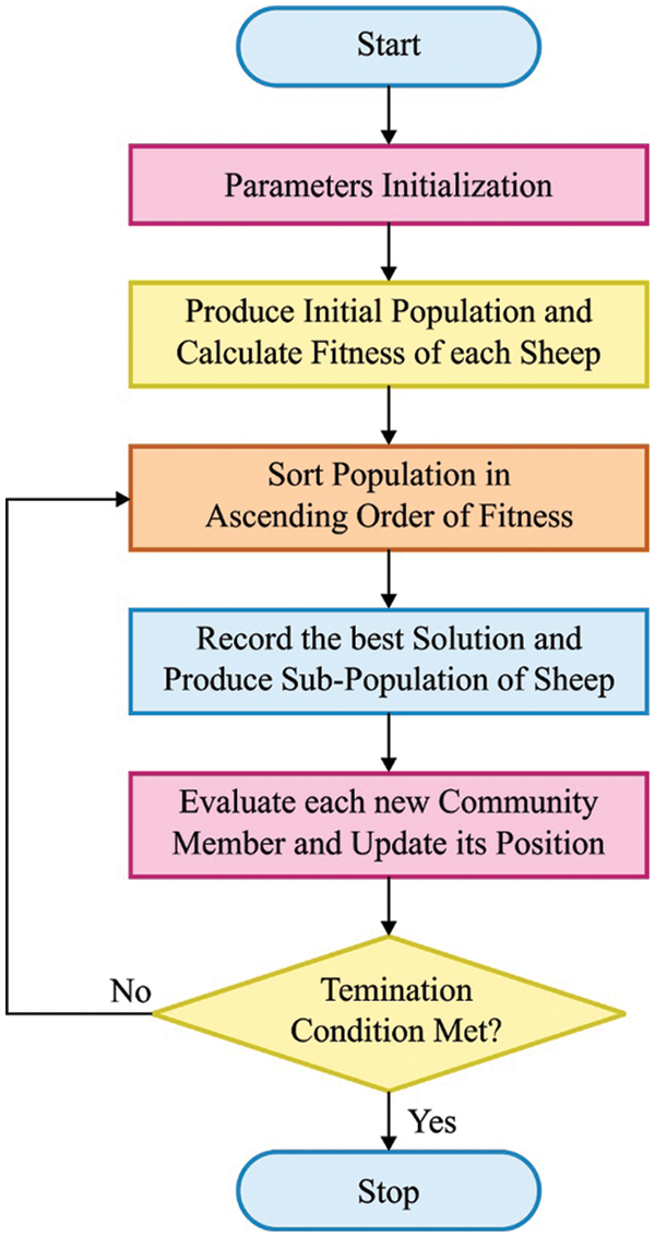
Figure 3: Flowchart of SSO

4  Performance Validation

The proposed INS-ODBN technique was evaluated for its performance against benchmark MESSIDOR dataset [27]. Fig. 4 displays some of the test fundus images. Fig. 5 depicts the samples results for qualitative analysis, accomplished by INS-ODBN model. Fig. 5a showcases the original retinal fundus image and Fig. 5b illustrates the segmented versions of the input fundus images. At last, Fig. 5c depicts the classified fundus image.

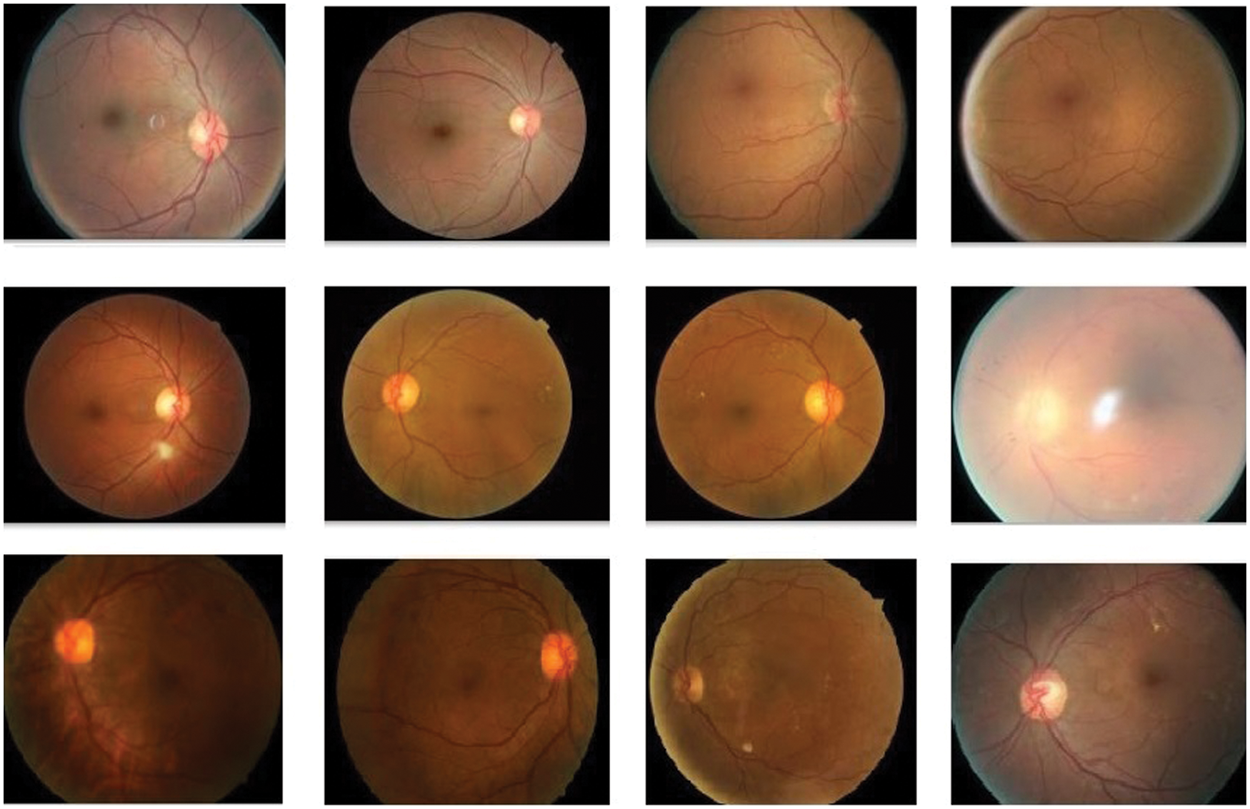
Figure 4: Sample images

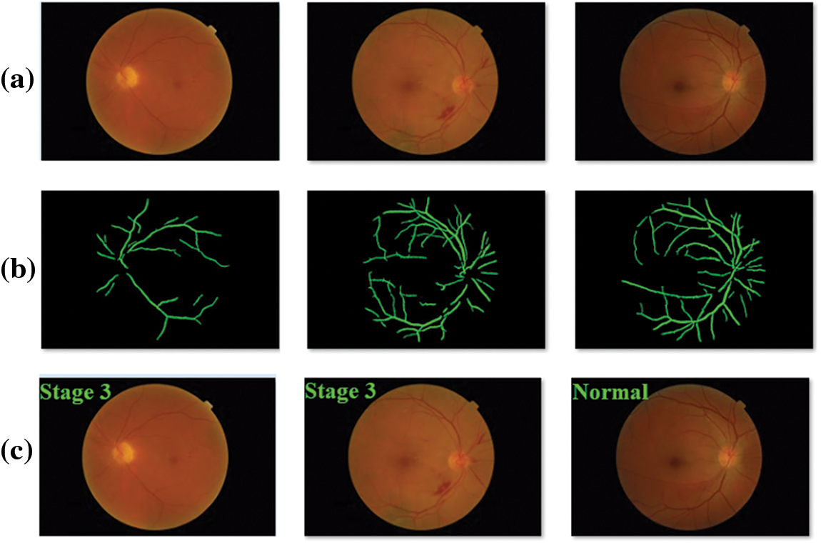
Figure 5: Sample results (a) first row-input image (b) second row-segmented output (c) third row-classified output

Tab. 1 and Figs. 6–7 shows the results from DR detection analysis, achieved by INS-ODBN model on test images. The proposed INS-ODBN model categorized the ‘Normal’ class images with a sens_y of 94.89%, spec_y of 97.34%, prec_n of 97.44%, and an acc_y of 97.45%. Meanwhile, the proposed INS-ODBN approach classified the ‘Stage 1’ class images with a sens_y of 95.23%, spec_y of 98.13%, prec_n of 96.18%, and an acc_y of 95.42%. Eventually, INS-ODBN technique identified the ‘Stage 2’ class images with a sens_y of 96.86%, spec_y of 98.21%, prec_n of 97.97%, and an acc_y of 96.61%. Finally, the presented INS-ODBN method categorized the ‘Stage 3’ class images with a sens_y of 96.87%, spec_y of 98.65%, prec_n of 95.38%, and an acc_y of 96.83%.

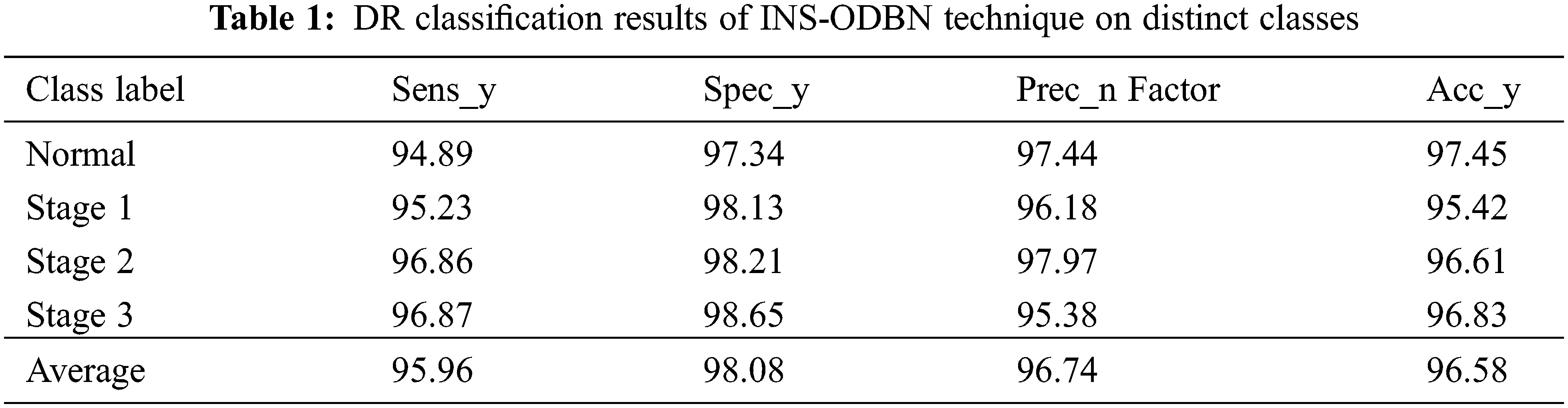
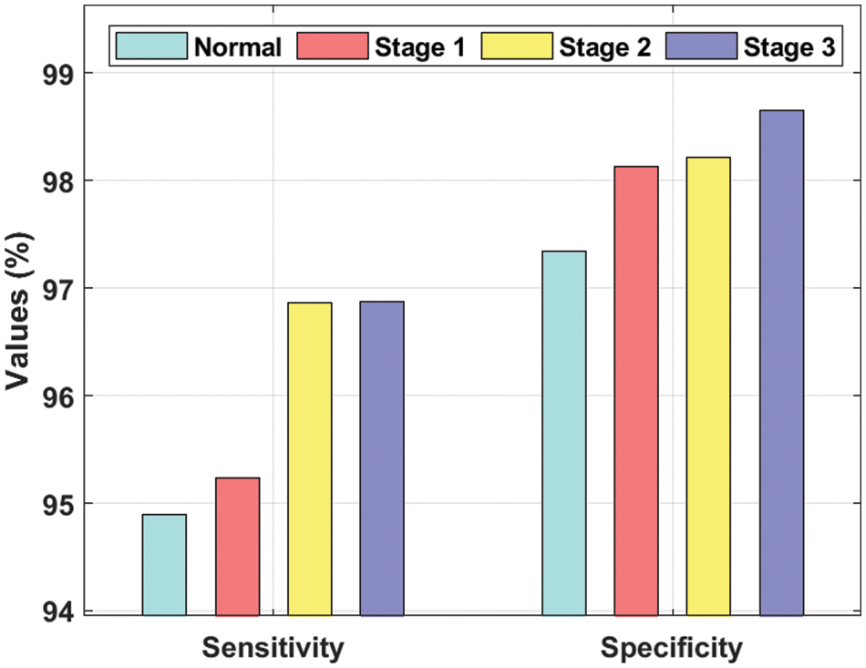
Figure 6: Sens_y and spec_y analysis of INS-ODBN method

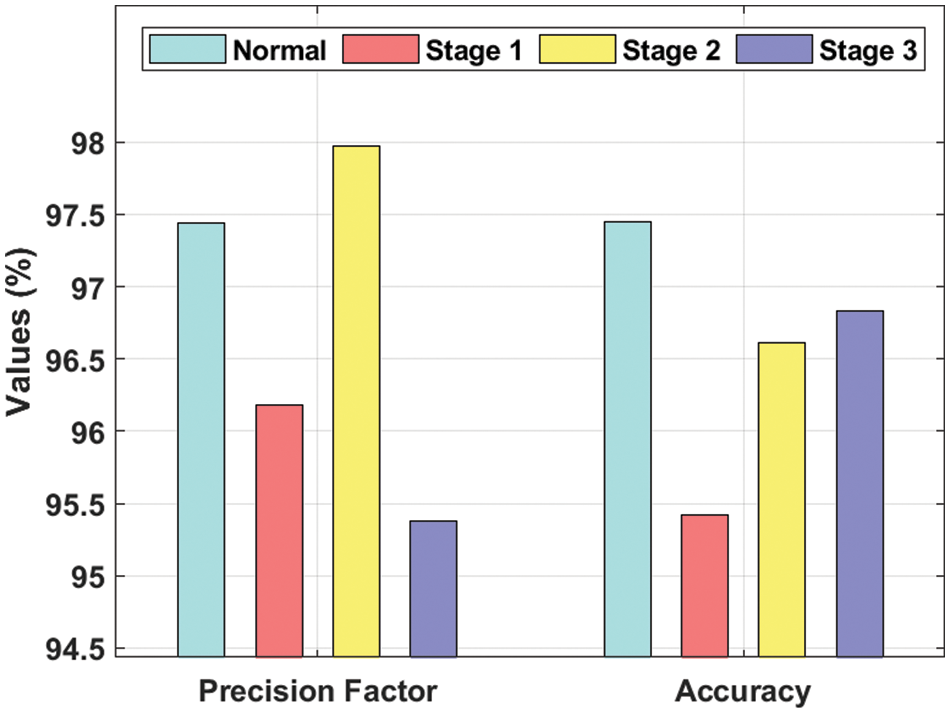
Figure 7: Prec_n and acc_y analysis of INS-ODBN method

Fig. 8 exemplifies the average DR detection analysis results accomplished by the proposed INS-ODBN model. The experimental values portray that INS-ODBN technique produced the maximum average sens_y of 95.96%, spec_y of 98.08%, prec_n of 96.74%, and an acc_y of 96.58%.

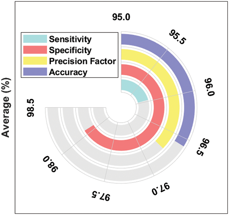
Figure 8: Average analysis results of INS-ODBN method with distinct metrics

On the other hand, ResNet and Human models produced manageable results such as spec_y of 90.53% and 93.20% respectively. VggNet-s and VggNet-19 models attained reasonable spec_y values such as 93.98% and 96.05% correspondingly. But, the proposed INS-ODBN algorithm accomplished supreme outcomes with a spec_y of 98.08%.

Fig. 9 offers the sens_y examination results achieved by INS-ODBN model against recent techniques [28–30]. The results display that VggNet-s and AlexNet models attained the least sens_y values such as 33.43% and 39.12% respectively. Next to that, VggNet-19 and Binary DT models showcased slightly enhanced sens_y values such as 54.51% and 58.18% respectively. Then, GoogleNet and ResNet models demonstrated moderate sens_y values such as 64.83% and 73.77% respectively. Afterward, Polynomial-Kernel Support Vector Machine (KSVM) and Radial Basis Function (RBF)-KSVM models produced manageable sens_y values like 80.91% and 81.82% correspondingly. Meanwhile, VggNet-16 and human models attained reasonable sens_y values such as 86.37% and 86.4% respectively. However, the presented INS-ODBN technique accomplished a superior outcome with a sens_y of 95.96%.

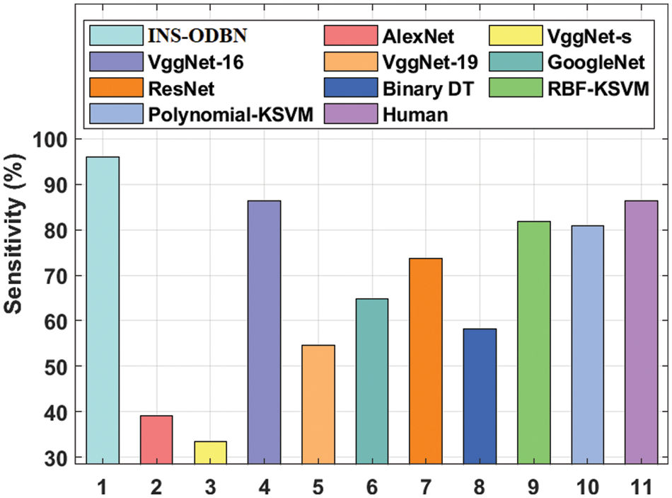
Figure 9: Comparative analysis results of INS-ODBN model in terms of sens_y

Fig. 10 shows the spec_y analysis results accomplished by INS-ODBN approach against existing models. The resultant values reveal that VggNet-16 and Polynomial-KSVM models attained the least spec_y values such as 29.09% and 55.45% correspondingly. Binary DT and GoogleNet techniques showcased slightly improved spec_y values such as 80.43% and 86.84% correspondingly. Further, AlexNet and RBF-KSVM models too demonstrated moderate spec_y values such as 90.07% and 90.43% respectively.

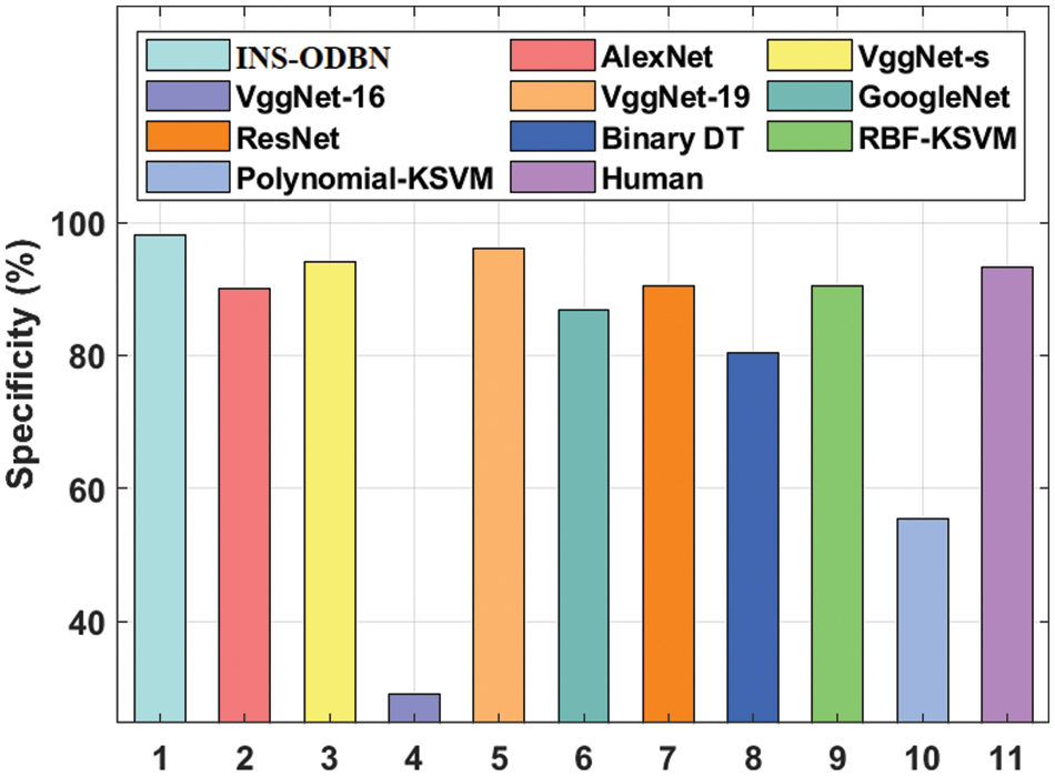
Figure 10: Comparative analysis results of INS-ODBN model in terms of spec_y

Fig. 11 showcases the acc_y analysis results produced by INS-ODBN method against other techniques. The results exhibit that VggNet-16 and Polynomial-KSVM models attained the least acc_y values such as 48.13% and 68.18% respectively. Next to that, AlexNet and VggNet-s models showcased slightly enhanced acc_y values such as 73.04% and 73.66% respectively. Next, ResNet and Binary DT techniques demonstrated moderate acc_y values namely, 78.68% and 79.09%. Afterward, VggNet-19 and GoogleNet methods produced manageable acc_y values such as 82.17% and 86.35% respectively. In the meantime, Human and RBF-KSVM models too produced reasonable acc_y values such as 90.20% and 90.91% respectively. However, the projected INS-ODBN methodology outperformed other methods and accomplished the maximum results with an acc_y of 96.58%.

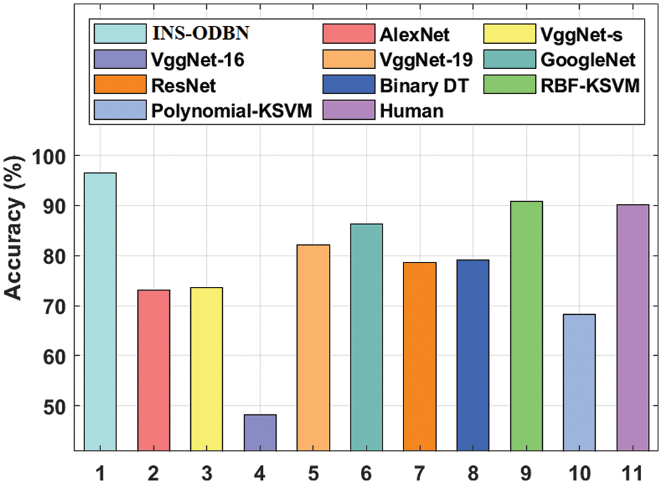
Figure 11: Comparative analysis results of INS-ODBN model in terms of acc_y

5  Conclusion

The current study has developed an IoT-enabled DR disease diagnosis method using INS-ODBN model. Once the DR images are preprocessed, INS method is utilized for the detection of diseased regions in input fundus images. Then, the feature extraction process takes place using histogram features, texture features, and wavelet features which derive a set of features for classification process. Finally, at the time of image classification, ODBN model is implemented in which the parameter tuning of DBN model is carried out by SFO algorithm. The presented model was evaluated through experiments using benchmark DR dataset and the outcomes were validated under different performance measures. The resultant values demonstrate that the proposed INS-ODBN technique yields better efficiency over existing approaches. In future, DR detection efficiency of INS-ODBN technique can be enhancing using DL-based feature extractors.

Funding Statement: The authors received no specific funding for this study.

Conflicts of Interest: The authors declare that they have no conflicts of interest to report regarding the present study.

This work is licensed under a Creative Commons Attribution 4.0 International License, which permits unrestricted use, distribution, and reproduction in any medium, provided the original work is properly cited.