Computer Systems Science & Engineering DOI:10.32604/csse.2023.026582
Article

A Novel Segment White Matter Hyperintensities Approach for Detecting Alzheimer

Antonitta Eileen Pious1,* and U. K. Sridevi2

1Department of Science and Humanities, Sri Krishna College of Engineering and Technology, Coimbatore, 641008, India
2Department of Applied Mathematics and Computational Sciences, PSG College of Technology, Coimbatore, 641008, India
*Corresponding Author: Antonitta Eileen Pious. Email: eileenpious@gmail.com
Received: 30 December 2021; Accepted: 06 April 2022

Abstract: Segmentation has been an effective step that needs to be done before the classification or detection of an anomaly like Alzheimer’s on a brain scan. Segmentation helps detect pixels of the same intensity or volume and group them together as one class or region, where in that particular region of interest (ROI) can be concentrated on, rather than focusing on the entire image. In this paper White Matter Hyperintensities (WMH) is taken as a strong biomarker that supports and determines the presence of Alzheimer’s. As the first step a proper segmentation of the lesions has to be carried out. As pointed out in various other research papers, when the WMH area is very small or in places like the Septum Pellucidum the detection of the lesion is hard to find. To overcome such problem areas a very optimized and accurate Threshold would be required to have a precise segmentation to detect the area of localization. This would help in proper detection and classification of the Anomaly. In this paper an elaborate comparison of various thresholding techniques has been done for segmentation. A novel idea for detection of Alzheimer’s has been presented in this paper, which encompasses the effectiveness of an optimized and adaptive technique. The Unet architecture has been taken as the baseline model with an adaptive kernel model embedded within the architecture. Various state-of-the-art technologies have been used with the dataset and a comparative study has been presented with the current architecture used in the paper. The lesion segmentation in narrow areas has accurately been detected compared to the other models and the number of false positives has been reduced to a great extent.

Keywords: Alzheimer’s; adaptive threshold; deep learning; segmentation

1  Introduction

Thresholding has been a technique used for a very long time to separate parts of an image based on some value, this helps segment the image and allows the Region of Interest (ROI) to be concentrated upon [1]. It also equips us from clearly differentiating the fore ground of an image from the background. In the detection of Alzheimer’s this is a very crucial part as the area where the lesion lies is segmented and helps in tracing the level of abnormality present. Thresholding techniques play a vital part of any segmenting process and are usually considered as the first step of segmenting. When we consider WMH as a strong biomarker in detecting Alzhemier’s [2], a proper threshold value to correctly segment the area of lesion occurrence is mandatory. Thresholding can be performed in the following ways depending on what kind of data they are dealing with or working on. The Tab. 1 below gives us a broad classification of the various thresholding techniques used.

The purpose of segmentation is to choose characteristics of our choice, as in this case the hyperintensity level to be more localized which in turn aids in the proper classification and detection of Alzheimer’s. Automated segmentation in an aging brain becomes very complex to process because of the heterogeneous nature of WMH [9].

The lesser the threshold, the more homogeneous the segments will be. A larger threshold value will cause a more heterogeneous and generalized segmentation result. Every image is made up of a collective group of pixels values. In image segmentation the task is to classify the image into various segments depending on the classes assigned to the pixel value. Processing the entire image doesn’t serve any fruitful purpose, So segmenting pixels on an apt threshold value helps us in detecting WMH areas that are usually missed out. Thresholding is a type of segmentation where we change the pixels of an image to make the image easier to analyze. The school old methods of thresholding like Otsu’s Thresholding [10], adaptive thresholding, and grab cut thresholding methods were used with the dataset to help gain a better understanding of the optimized threshold value. The drawback of Otsu’s thresholding of WMH was the inability of the method to detect the number of occurrences of the false positives because of the heterogenous nature of the pixels [11] Otsu’s thresholding technique would have been suitable for a bimodal image. The histograms that were displayed for the noisy images fed, did not serve the purpose and the peak of thresholding wasn’t visible enough. Next the adaptive thresholding technique was utilized with multiple thresholds this was apt when dealing with the varying intensities of WMH. But the disadvantage of adaptive thresholding was that the size of the neighborhood had to be large enough to cover sufficient foreground and background pixels, otherwise a poor threshold was chosen. In the case of WMH, the pattern of occurrence is very hazy and hard to identify [12]. The grabcut segmentation worked fairly well but required the ROI to be specified. This study as shown in Fig. 1 helped us gain an insight that deep learning models would be well suited for the automatic detection of features and to increase the accuracy of segmentation and speed.

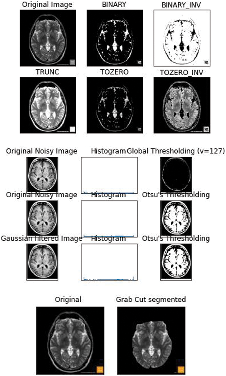
Figure 1: 2D FLAIR image from the WMH dataset was fed and the basic thresholding methods were performed on it

2  Materials and Methods

2.1 Materials Used

The dataset used in this paper was got from the WMH segmentation challenge. The medical images used were collected from five different scanners from hospitals in Netherland and Singapore. Both 3DT1 and FLAIR images were used. Elastix 4.8 a toolbox for medical image registration was used for the alignment of 3DT1 with FLAIR images. The images were preprocessed using SPM12r6685 to correct the bias field inhomogenities using statistical parameter mapping.

2.2 Preprocessing

We further pre processed the raw data to serve our purpose of removing false positives, the segmentation of the non brain tissues from the actual brain tissues is a tremendous task for clinicians too. The available dataset from the WMH segmentation challenge is 3D T1-weighted sequence consisting of 192 slices, each slice having a voxel size: 1.00 × 1.00 × 1.00 mm3. The dataset also has a 3D FLAIR sequence of 321 sagittal slices, voxel size: 1.04 × 1.04 × 0.56 mm3. Each folder contains 3 types of images in Nifti format. The NiBabel package was used to load the images into the Python software. Three variables were used to differentiate the images as-T1weighted: This is the raw MRI image with a single channel. The Images in the dataset are 3D and can be imagined as multiple 2D images stacked together. T1w_brainmask: It is the image mask of the brain or can be called as the ground truth. It is obtained using Extractor tool from the deepbrain 0.1 library. T1w_brain: This can be thought of as part of brain stripped from above T1weighted image. This is similar to overlaying mask to actual images. A Skull extraction was performed to help remove the non brain areas from the brain areas [13] as shown in Fig. 2. The GPU environment used was the Google Colaboratory.

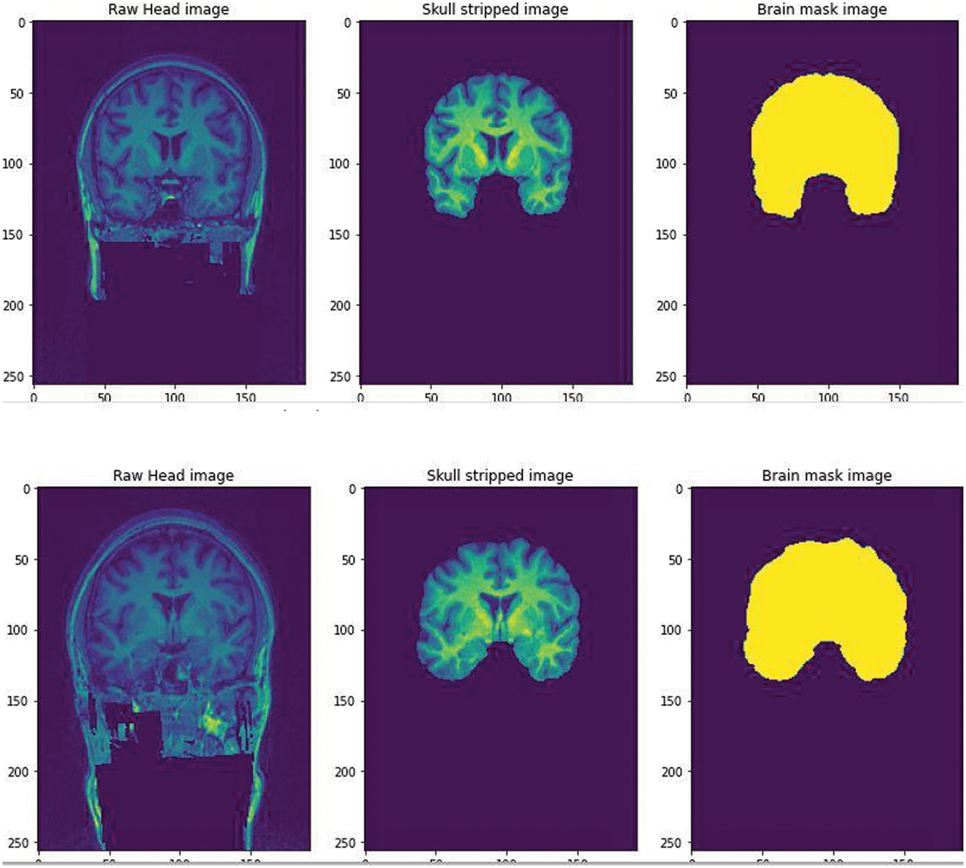
Figure 2: The Raw image from the WMH dataset was fed and skull stripped using the Extractor tool from deepbrain library. A brain mask image was created to help train the CNN for a predicted output

A simple CNN architecture [14] was used to create a mask to train the model in predicting the skull stripped image. After training for 60 epochs we got a validation Intersection over Union (iou_score) of 0.88, the result obtained is shown in Fig. 3. The iou_score helped in identifying the quantification of overlap between the target mask and the prediction image.

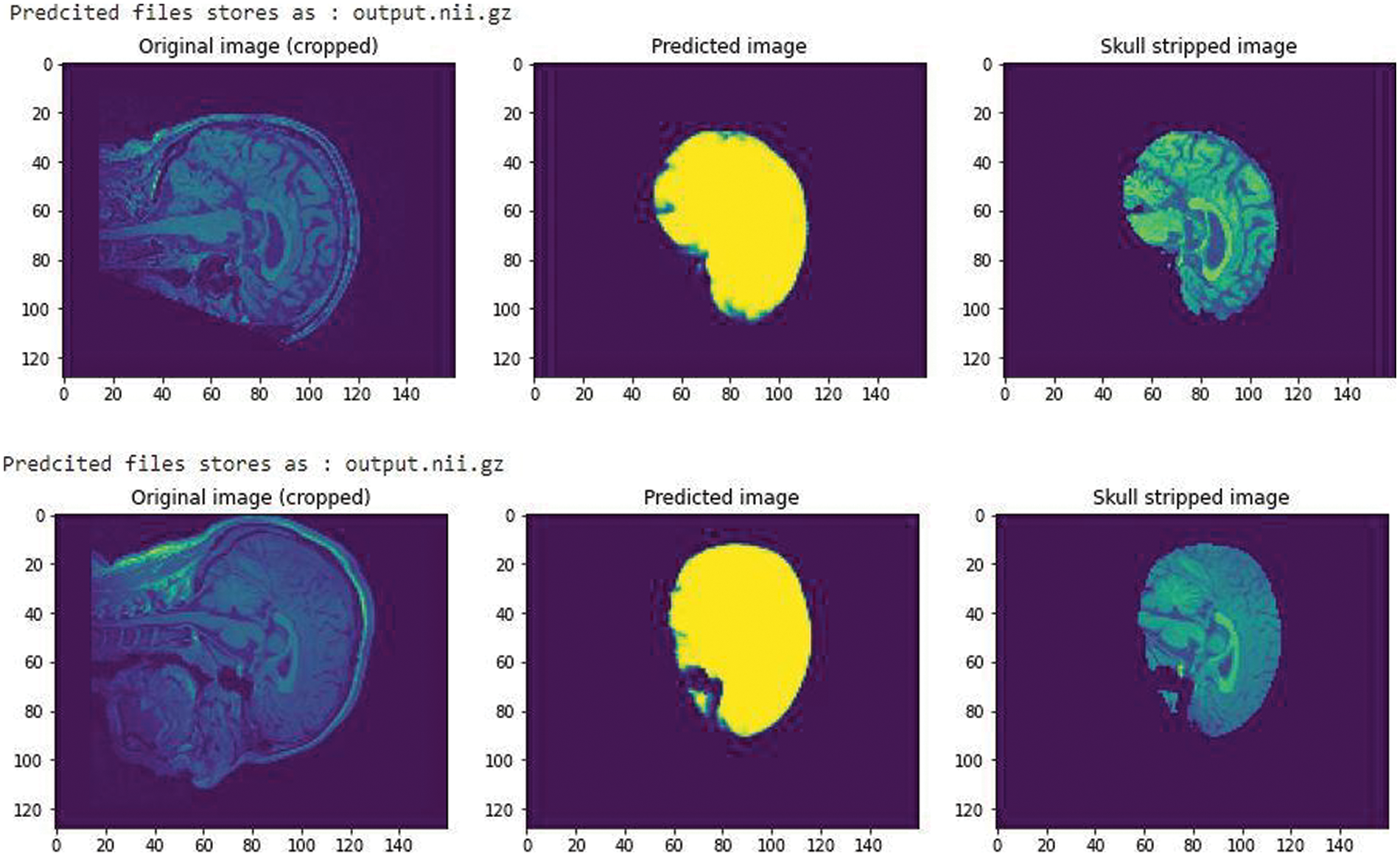
Figure 3: A CNN trained model with an iou_score of 0.88 after training for 60 epochs

All images were pre-processed with N4ITKBiasFieldCorrection [15] to correct bias field inhomogeneities.

Figure 4: Bias field correction

3  Network Architecture

3.1 Baseline Model

In the current study, we put forth our work to combine an adaptive thresholding strategy with a 3D Unet architecture [16]. In the previous research studies as we have seen the Smaller WMH were difficult to trace out and the detection of false positives in areas like the Septum Pellucidum was really very difficult to comprehend. According to our method used here, we make use of the Unet architecture which holds well in downsampling an image concentrating on the spatial dimensions and localization. Unlike CNN architecture which is quite suitable to only detect the presence or absence of a morbidity, the Unet architecture helps to classify the morbidity as well as trace the area where they are present by segmenting each and every pixel in the ROI (Region of Interest). The second reason of choosing a Unet is the availability of images of arbitrary sizes, which requires an architecture which would accept a heterogeneous kind. A general Unet architecture makes use of skip connections between the contracting and the expanding path in order to recover spatial information lost during down sampling. Or in other words it helps in removing the vanishing gradient problem. Here, we further advance 3D Unet for WMHs segmentation (Fig. 5) with two original components: A use of different details for the network architecture and inclusion of a threshold of pixilated values that are concatenated with the up sampled values.

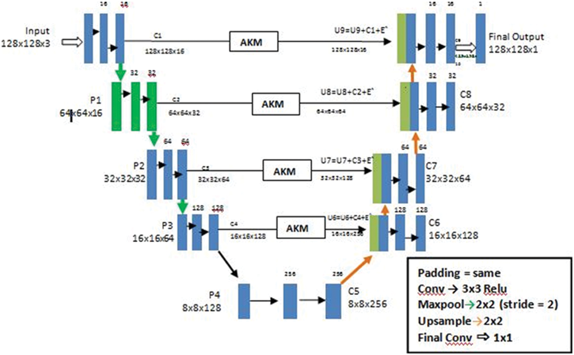
Figure 5: The architecture of a U-Net AKM model

3.2 Adaptive Kernel Model

Our primary goal is to make the architecture less location sensitive that is it should not reject or not detect a White Matter Hyperintensity in a low probability area like the Septum Pellucidum. Our second goal is ultimately to reduce the false positives for this we have used an Adaptive kernel model in between the skip connections of the encoder and decoder. The Adaptive Kernel Model (AKM) basically gets the feature map with a large receptive field from the encoder and performs an adaptive thresholding on it using a 3 × 3 and 5 × 5 kernel achieving the best result. The strategy used here was to give the integral image as input and figure the left and above pixel values, as shown in Fig. 6.

I(x,y)=f(x,y)+I(x−1,y)+I(x,y−1)−I(x−1,y−1) (1)

Once we have the innate image, the sum of the function for any rectangle with upper left area (x1, y1) and lower right area (x2, y2) can be computed in constant time using the following equation

∑x=x1x2⁡∑y=y1y2⁡f(x,y)=I(x2y2)−I(x2,y1−1)−I(x1−1,y2)+I(x1−1,y1−1) (2)

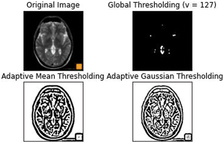
Figure 6: An Adaptive mean and Gaussian thresholding applied with an approximate threshold value of around 127

This thresholding technique helps in discriminating the higher and lower intensity areas of white matter. The output of A3 and A5 are fed into an element wise sum function, followed by a fully connected layer Fmp to carry out an accurate and localized selection. The resulting feature map contains the determined weights for White Matter of different intensities. This being a binary classification problem a sigmoid function is made use of, the parameters are then applied to each feature map and all of them are summed up as follows. The output of values is concatenated alone with the down sampled values. The inclusion of the AKM unit as shown in Fig. 7 has helped discern the difference in intensities to a larger extent with a focus on areas with meager existence of White matter like the Septum Pellucidum.

E^=A3^+A5^=a.A3+b.A5 (3)

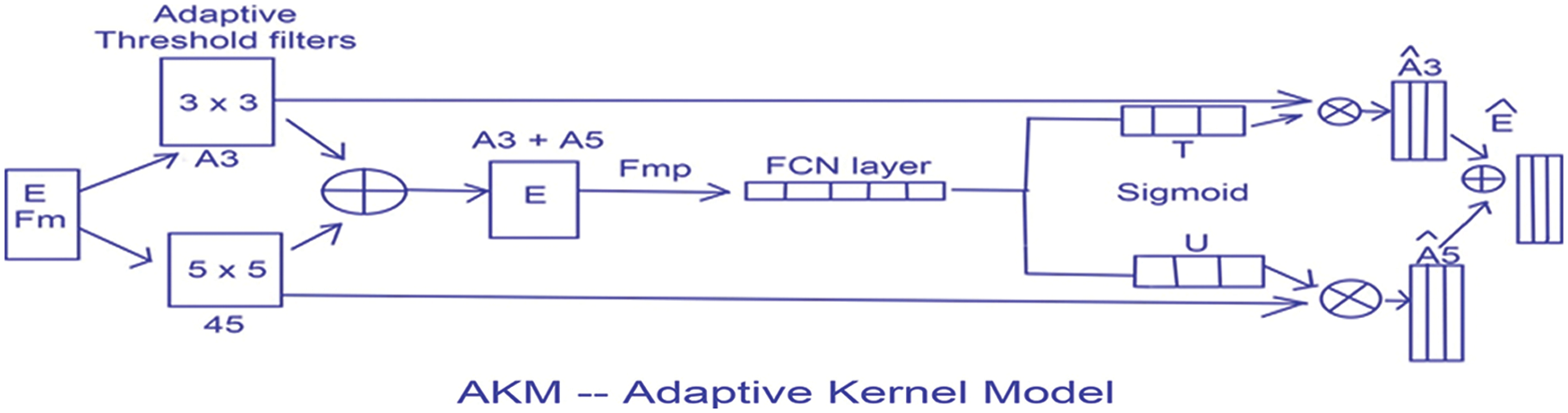
Figure 7: The AKM model architecture

4  Experiments and Results

The metrics to assess our proposed method were selected from the suggestion of the MICCAI 2017 challenge, which included the Dice Similarity Coefficient, Hausdroff distance, Absolute percentage Volume difference, the sensitivity for detecting individual lesions (recall) and F1 score for individual lesions (F1)

They are defined in the Equations given below to suit our requirement of tracing WMH.

Dice Similarity coefficient (DSC) [17] can be calculated as follows

DSC=2∗TP2∗TP+FP+FN (4)

Hausdroff distance (HD) helps to calculate the distance of a point (m) in the model image to the point in the tested image (s). A HD of values closer to zero indicates a partial matching while a value equal to zero tells us the ground image and segmented image have totally matched. We have used the following formula in calculating the Hausdroff distance here

M={m1,m2_______________mp} (5)

S={s1,s2_____________________s3} (6)

H(M,S)=max(h(M,S),h(S,M) (7)

where

h(S,M)=maxm∈Mmins∈S‖m−s‖ (8)

Absolute percentage Volume difference (AVD) [18] can be calculated as the absolute log value of the segmented volume divided by the true volume.

AVD=|logSegmentedvolumeofimageTruevolumeofimage| (9)

The recall or sensitivity can be defined as the true positive rate (TPR) [18], it measures the number of positive voxels in the expected image that are also identified as positive in the segmented image.

Recall=TPR=TPTP+FN (10)

And the final metric of assessment we use here is the precision or F1 score [18] which can be calculated as

F1=TPTP+1(FP+FN)2 (11)

From the above equations TP-True Positive

TN - True Negative

FP - False Positive

FN - False Negative

5  Implementation Details

Our proposed architecture was implemented with the Python and Keras framework. We make use of the U-Net architecture as the base structure of the auto encoder-decoder framework. Since the images in the dataset have a heterogeneous resolution, we perform the pre processing techniques like skull stripping and bias correction. The parameters vary depending on the heterogeneity of the images available. The input taken was 128 × 128 matrix for an 3 channel input, with a convolutional layer of 3 × 3, a maxpooling of 2 × 2 and a stride of 2. We make use of the ADAM optimizing algorithm with a batch size of 32 and epochs of 30. The initial learning rate is set at 0.00003 and is dropped by 10 percent after each 30 epochs.

6  Results

According to the observations White Matter intensities in areas like the Septum pellucidum were hard to trace out because of the variability in intensities and volume. Here in our proposed method a 3D multislice attainment is made with relatively few slices for training the Unet architecture. As per the requirement the number of false positives of the White Matter Hyper intensities in smaller regions had to be segmented perfectly well. The combined approach of using an Adaptive thresholding method to the feature map received from the encoder to the decoder helped in bringing the recall and F1 rate to 0.86 and 0.80 respectively. This change in values implies the decrease in the false positive pixel values and the overall accuracy has improved extensively as shown in Fig. 8.

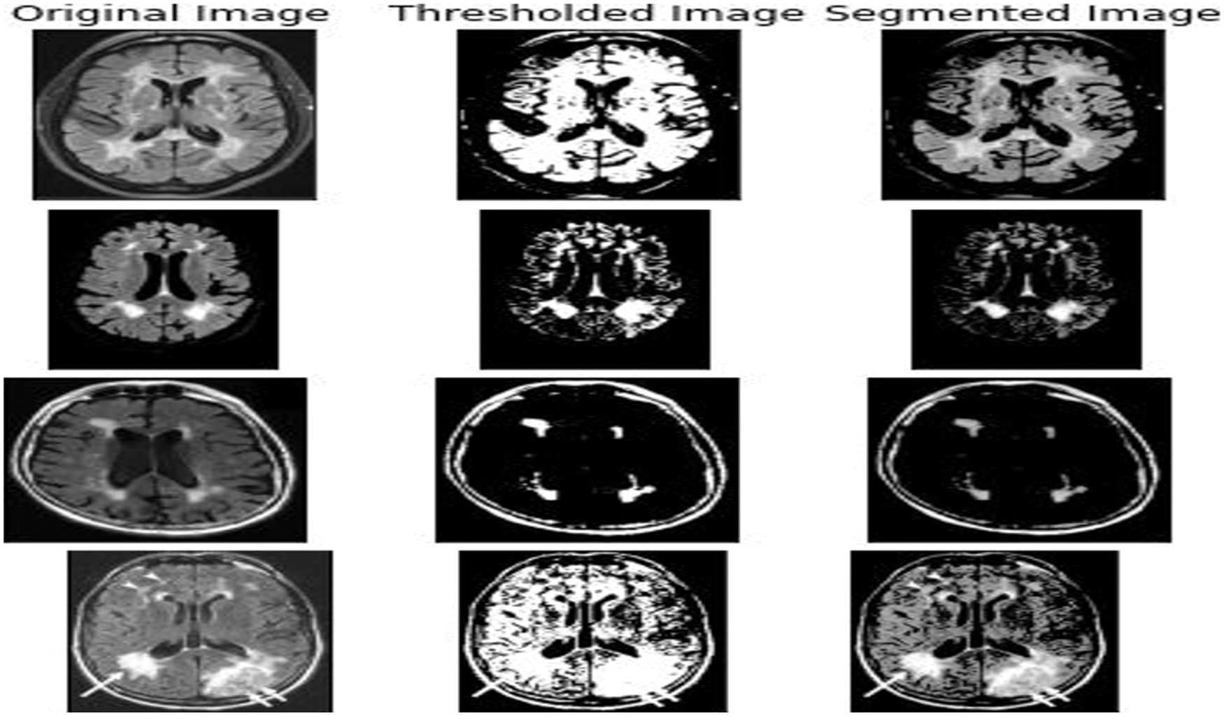
Figure 8: The output got from various input images like the 3DT1 and 3D Flair images that were fed into the Unet AKM model

The overall accuracy of the proposed model has turned out to be around 0.75 iou_score for 120 epochs. From the plot of accuracy Fig. 9 the model could most likely be trained a little more as the trend for accuracy on both datasets is still rising for the last few epochs. It can be noticed that the model has not yet over-learned the training dataset, showing similar ability on both datasets using for training and testing. From the plot of loss, the model has an optimal performance on both train and validation datasets (labeled test). If these parallel plots start to depart consistently, it might be an indication to stop training at an earlier epoch.

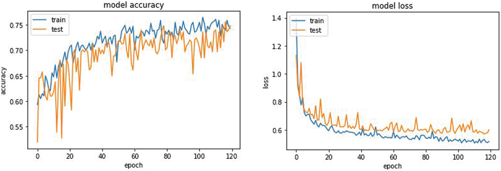
Figure 9: Model accuracy and model loss of the Unet AKM model

7  Comparison with Other Published Methods

A comparative study was done with three frameworks as shown in Tab. 2 like the fully convolutional neural network with an ensemble of three different networks and three different initializations of weight. A data normalization and augmentation was applied to remove the false positives. The second framework that was used as a comparative model was a multi dimensional gated recurrent unit. And the third framework that was used for a comparative study was a multi scale deep network with annealed training with a patch based architecture, where patches of sizes 128 × 128, 64 × 64 and 32 × 32 were extracted and fed into a deep convolutional network [19] as shown in Fig. 10.

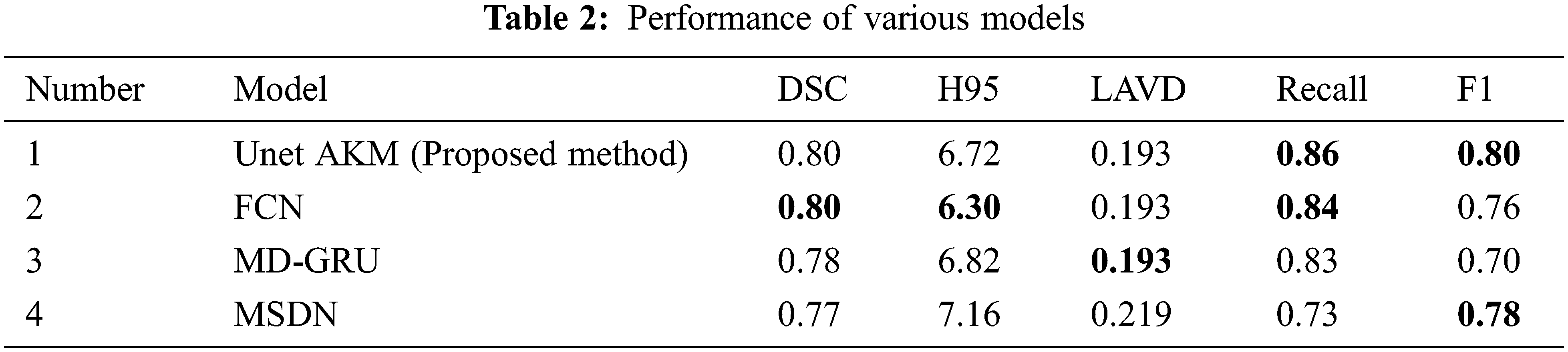
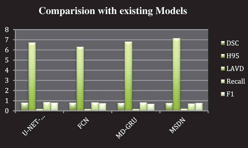
Figure 10: Comparison with other existing models

8  Conclusion

Our proposed work has helped reduce the occurrence of false positives and improve the accuracy rate compared to the already existing Deep learning framework. It has also helped in detecting the presence of WMH in smaller regions like the Septum Pellucidum. Further work can involve the inclusion of volume and shape of the WMH along with the intensity changes. This would help to unravel the actual presence of WMH and the extent of the spread of the morbidity. This would help clinicians with a more clear and precise view in the detection of Alzheimer’s.

Funding Statement: The authors received no specific funding for this study.

Conflicts of Interest: The authors declare that they have no conflicts of interest to report regarding the present study.

This work is licensed under a Creative Commons Attribution 4.0 International License, which permits unrestricted use, distribution, and reproduction in any medium, provided the original work is properly cited.