Computer Systems Science & Engineering DOI:10.32604/csse.2023.026810
Article

Availability Capacity Evaluation and Reliability Assessment of Integrated Systems Using Metaheuristic Algorithm

A. Durgadevi* and N. Shanmugavadivoo

Department of Electrical and Electronics Engineering, Thiagarajar College of Engineering, Madurai, 625015, India
*Corresponding Author: A. Durgadevi. Email: durgadevi.tneb@gmail.com
Received: 05 January 2022; Accepted: 23 February 2022

Abstract: Contemporarily, the development of distributed generations (DGs) technologies is fetching more, and their deployment in power systems is becoming broad and diverse. Consequently, several glitches are found in the recent studies due to the inappropriate/inadequate penetrations. This work aims to improve the reliable operation of the power system employing reliability indices using a metaheuristic-based algorithm before and after DGs penetration with feeder system. The assessment procedure is carried out using MATLAB software and Modified Salp Swarm Algorithm (MSSA) that helps assess the Reliability indices of the proposed integrated IEEE RTS79 system for seven different configurations. This algorithm modifies two control parameters of the actual SSA algorithm and offers a perfect balance between the exploration and exploitation. Further, the effectiveness of the proposed schemes is assessed using various reliability indices. Also, the available capacity of the extended system is computed for the best configuration of the considered system. The results confirm the level of reliable operation of the extended DGs along with the standard RTS system. Specifically, the overall reliability of the system displays superior performance when the tie lines 1 and 2 of the DG connected with buses 9 and 10, respectively. The reliability indices of this case namely SAIFI, SAIDI, CAIDI, ASAI, AUSI, EUE, and AEUE shows enhancement about 12.5%, 4.32%, 7.28%, 1.09%, 4.53%, 12.00%, and 0.19%, respectively. Also, a probability of available capacity at the low voltage bus side is accomplished a good scale about 212.07 times/year.

Keywords: Meta-heuristic algorithm; modified salp swarm algorithm; reliability indices; distributed generations (DGs)

1  Introduction

The primary function of any electric power system network is to supply energy to its consumers at optimum operational costs by warranting superior quality and continuity at all eras [1]. Due to the continual growth of populations and industrial expansions, the consumption degree of electricity rises promptly every year, which upsets the ecological factors and leads to reliable abridged operation [2–6]. Recently, distributed generations are regarded as the key trends among the researchers that offer several benefits to the existing power system. However, integrating energy systems requires coordinating various energy resources, particularly at urban locations [7]. The coordination and optimization of integrated energy systems offer novel solutions to existing problems that enhance energy efficiency and reliable operation. The influence level of the integrated/extended network, which includes the generation and transmission section and substation on the distribution section, shows the most significant importance in determining the power network extension. The new installation of the generation and transmission section requires a very high capital investment, and any outages in those sections lead to catastrophic consequences that impact socio-economic terms [8]. To overcome this, reliability assessment of the integrated or extended system needs to be carried out because reliability is the probability that the power system can accomplish its function satisfactorily deprived of any failure exposing to the operating conditions [9].

Generally, two approaches are adapted for reliability assessment of a power network, such as simulation and analytical [10,11]. From these evaluations, the obtained indices indicate the level of reliable operation of a distributed network section, and it doesn’t reflect on the whole network section or main grid of the power system. Due to this, the reliability assessment is challenging to apply the synchronizing operation and planning of a power network [12,13]. For better reliability, assessment with the computational efficiency of a whole power network using minimum cut-set procedure can be adapted. In addition to the minimum cut-set approach for a power network, the feeder partition procedure may be introduced in the distribution and substation section [14]. This work emphasizes evolving a reliability assessment for the integrated/extended power system in the presence of distributed generations such as Photovoltaic (PV), Wind turbine (WT), and Gas turbine (GT) that have the potential to reduce the power outage; one of the major concerns in the distribution system [15].

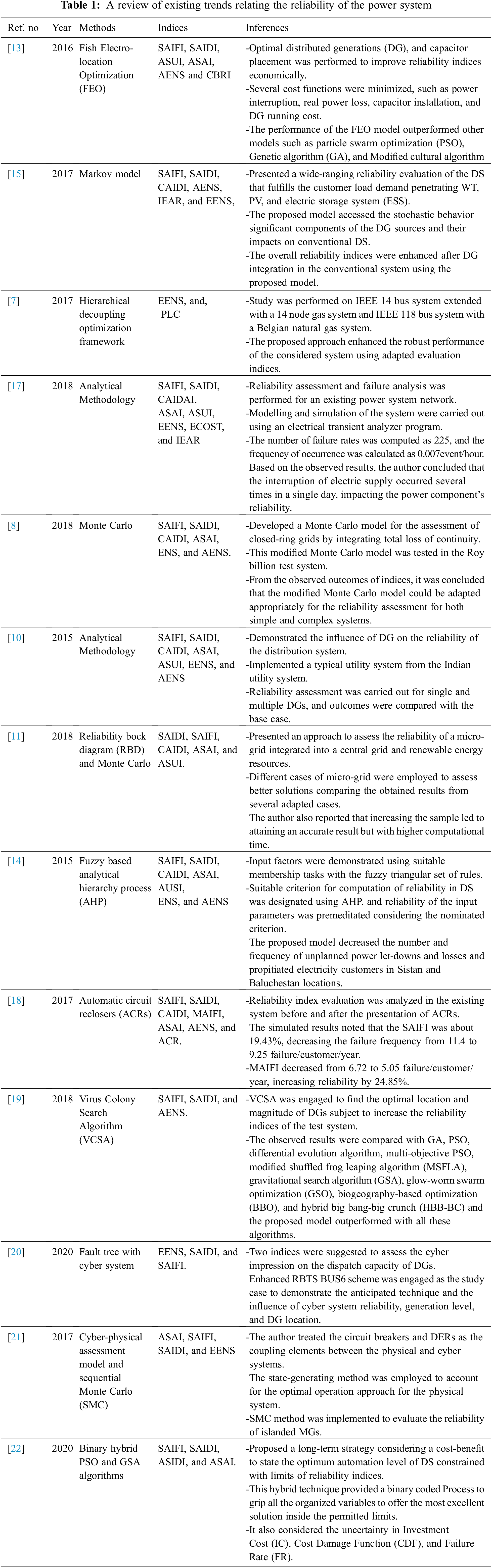
The distribution system (DS) contributes the highest proportion of power outages at the customer load points due to the radial nature of the network [16]. Hence, the reliability evaluation of the DS integrating with PV, WT, and GT has drawn more excellent responsiveness of many investigators. Considering all these facts, a substantial literature survey is carried out on the reliability assessment methodology used in the integrated power system in the following table (Tab. 1).

Based on the inferences from the intensive literature study, it is found that there are research gaps that need to be carried forward to find or enhance the solution further. Some of them are as follows,

•   Optimized reliability evaluation metrics are not significantly demonstrated.

•   Analytical approaches are adapted by several authors that lead to severe computation time.

•   Meta-heuristic approaches are not employed prominently for extended/integrated power networks.

•   Limited works are found that evaluate the reliability indices after integrating with renewable energy resources.

•   Most of the authors derived the reliability indices by segregating the whole system into several feeders.

•   There is evidence of limited consideration of reliability indices for integrated distributed systems.

Considering the research gaps mentioned-above, this work targets to derive the following objectives,

•   To evaluate the reliability of the extended power network integrated with Photovoltaic (PV), Wind turbine (WT), and Gas turbine (GT).

•   To compute the most optimized reliability indices using meta-heuristic algorithm i.e., Modified Salp Swarm algorithm.

•   To demonstrate various case studies considering the tie line operation of the extended system with the existing system.

•   To evaluate the penetration of distributed generations into the existing system using optimized reliability indices.

•   To assess the overall indices without classifying the feeder in the existing system.

The rest of the work is organized as follows: Section 2 demonstrated the problem formulation, proposed methodology, and case study used for the study. Subsequently, Section 3 illustrates the detailed results and discussions from the proposed model. Then, a comparative analysis is carried out between various cases and several existing methodologies in Section 4 that can validate the effectiveness of the proposed method. Finally, conclusions are made in Section 5 based on the observed results.

2  Proposed Methodology and Case Studies

2.1 Objective Function

The main three technical objective functions considered are minimizing the active power losses (PL) and Voltage Deviation (VD), and maximizing the Voltage Stability (VS) as detailed below [23]:

✓ The feeder system power losses (PL) can be minimized using Eq. (1)

PL=min(∑m=1nb⁡|Im2|∗Rm), (1)

where Im is the mth branch current magnitude, Rm is the resistance of mth branch, and nb is the total number of branches in the feeder system.

✓ The voltage deviation (VD) can be minimized by

VD=min(∑m=1NL⁡|Vr−Vm|), (2)

where NL is the total number of load buses, Vr is the rated voltage, Vm is the actual voltage magnitude at mth node.

✓ Maximization of voltage stability (VS) can be expressed as

VS=max{|Va4|−4(PbXab−QbRab)2−4(PbRab+QbXab)|Va|2 (3)

where Va denotes magnitude of the voltage at ath node, Pb and Qb are active and reactive power of the load at bth node, respectively, and Rab and Xab are the resistance and reactance of the line between the nodes a and b, respectively.

2.2 Constraints

The objective functions are subjected to the following operating constraints [23].

2.2.1 Equality Constraints

In a feeder system, the power balance constraints are as follows:

Psb+∑p=1NDG⁡PDGp=∑q=1nb⁡PLossq+∑q=1n⁡Pdq, (4)

Qsb+∑p=1NDG⁡QDGp=∑q=1nb⁡QLossq+∑q=1n⁡Qdq. (5)

where Psb and Qsb are active and reactive powers of the slack bus, respectively, PDGp and QDGp are the DG active and reactive power capacities at pth bus, respectively, PLossq and QLossq are the feeder active and reactive power losses of qth bus, respectively, Pdq and Qdq are the demanded active and reactive powers at qth bus, respectively, and ‘n’ is the total number of buses in the feeder system.

2.2.2 Inequality Constraints

✓ Generator performance constraints:

PDGmmin ≤PDGm≤PDGmmax, (6)

QDGmmin ≤QDGm≤QDGmmax. (7)

where PDGmmin and PDGmmax are minimum and maximum active power capacities of the DG at mth bus, and QDGmmin and QDGmmax are minimum and maximum reactive power capacities of the DG at mth bus, respectively.

✓ Capacity of DGs:

∑m=1NDG⁡PDGm≤PTD. (8)

where PDGm is real power fed by the DGs at the mth node, NDG is total number of DG units, and PTD is the total active power demand.

✓ Feeder voltage:

The feeder voltage constraints are stated as

Vmmin≤Vm≤Vmmax,m=1…NL (9)

where Vmmin and Vmmax are lowest and highest acceptable values of voltage at mth bus, respectively, Vm is load bus RMS voltage at mth bus, NL is the total number of load buses.

2.3 Modified Salp Swarm Algorithm

Modified Salp Swarm Algorithm (MSSA) mimics the swarming behavior of salps, and it is similar to jellyfishes that survive in the ocean as impelled through the body as propulsion to shift forward often appears as a flock called salp chain. These salp chains are classified into two groups such as leader and follower. Here the leader in the salp is present in front of the chain, and the remaining all salps are followers of the salp chain. A mathematical model for the position of the salp is defined in an m-dimensional exploration space where m is the number of variables in a given problem. Positions of all the salps are stored in a two-dimensional matrix called k. it is also assumed that there is a food source called f in the search space as the swarm’s target. In order to leader update the position of the leader, the following equation is expressed as:

km1={fm+c1((ubm−lbm)c2+lbm)c3≥0fm−c1((ubm−lbm)c2+lbm)c3≥0 (10)

where km1 shows the position of the first salp in nth dimension.

fm position of the food source in the nth dimension.

ubm upper bound of the nth dimension.

lbm lower bound of the nth dimension.

c1,c2andc3 are random numbers.

To update the position of the followers (Newton’s law of motion) is utilized, and it is expressed as follows:

kmi=12at2+vot (11)

where i ≥ 2, kmi shows the position of the ith follower in nth dimension.

t is time.

vo Initial speed

a=vfinalv0 and v=k−k0t .

The Modified Salp Swarm Algorithm (MSSA) algorithm modifies two control parameters of the actual SSA algorithm (Fig. 1). During the process of modification, a perfect balance between the exploration and exploitation phases will be maintained to ensure optimum solution of the objective function.

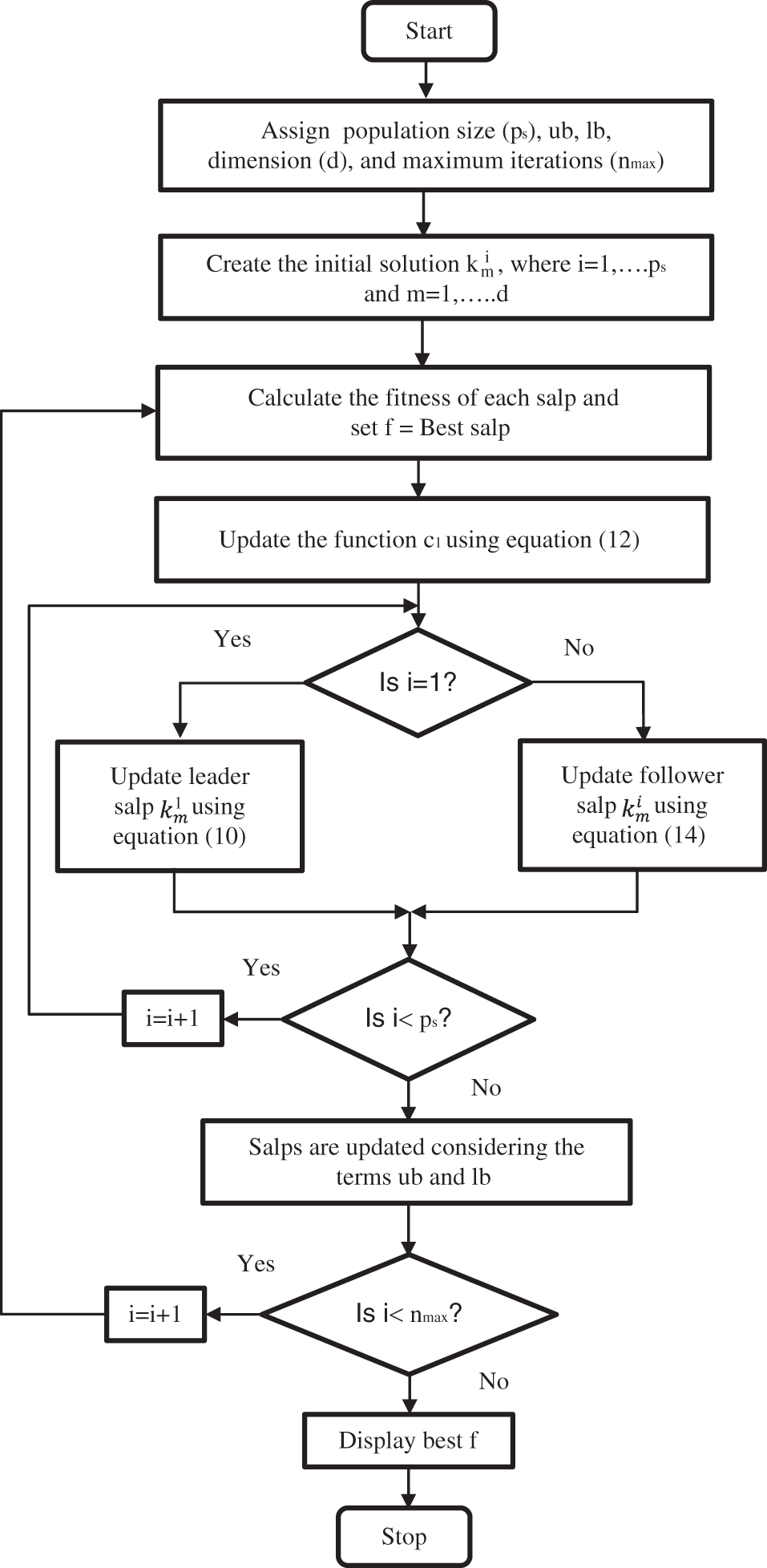
Figure 1: Flow chart of modified salp swarm algorithm

(1) In the actual SSA technique, the leader movement depends on the coefficient ( c1 ), the most significant parameter. It is slowly varied in earlier stages and rapidly in final stages which lowers the exploration capability of the SSA. The parameter c1 is calculated using the following equation,

c1=K1e−(4lL)2 (12)

where l and L represents the current iteration and the maximum no. of iteration, respectively. In the actual SSA algorithm, K1 represents the leader salp movement towards the food source, considered as 2. Higher value of K1 results in leader salp movement far off the food source. The value of K1 is set as 0.1 in the proposed MSSA. In the actual SSA, the variation of c1 is slow during start and fast during the last iterations which disappoints the normal process of any optimization algorithm. Also in SSA, the value of c1 is high during the end iteration compared to MSSA makes the leader position deviating widely from the food source. The other salps also face the same problem as they follow the leader salp. The above problems are solved during the final iteration with the new improved value of K1 .

(2) Also in SSA algorithm, the location of the follower salp is updated from its previous location as well as neighbourhood salp’s location as follows.

kmi=12(kmi+kmi−1)i≥2 (13)

where kmi and kmi−1 are the positions of ith and (i − 1)th salps in mth dimension. This eventually necessitates storing the position of ith and (i − 1)th salp after each iteration for calculating the next position of ith salp. It leads to extra computational time as well as additional memory requirement. It is to be noted that the location of any follower salp relies only on its previous location not on its neighbouring salp location. It has a direct impact on the exploitation ability of the algorithm. Consequently, Eq. (13) in the actual SSA algorithm is modified in such a manner that the successive position of the salp is always calculated from its previous location only as follows

kmi=14(kmi)i≥2 (14)

As the neighborhood follower salp’s location needs not to be saved, the modified equation reduces the execution time with minimum memory requirement. This in turn enhances the exploitation capability of the algorithm.

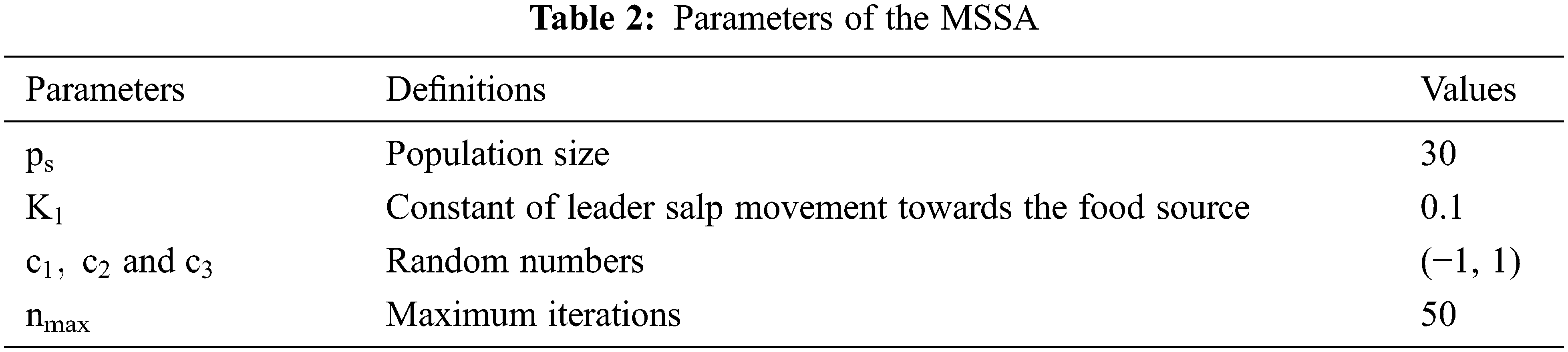
Though the global optimal of the optimization delinquent is unidentified, it can be presumed that the most satisfactory solution can be achieved through leader observation that travels towards the food source. Owing to this, the followers follow the assigned leader effectively. Consequently, as explained in the flowchart below, the salp chain attained supremacy to travel towards the global optimal circumstances but varying against diverse iterations [24]. The parameters of the MSSA are illustrated in Tab. 2 and MSSA algorithm is coded in MATLAB software environment and MATPOWER (an open-source software package) is used as a toolbox.

Considering the proposed methodology, this work targets the reliability assessment of the selected power system case studies, as illustrated in the following section.

2.4 Reliability Assessment Based MSSA Procedure

To evaluate the effectives of the proposed metaheuristic algorithm, the modified IEEERTS 79 test system extended with three feeder line IEEE 6 bus system shown in Fig. 2. It comprises 30 buses, 51 transmission lines, 36 generating units which are distributed among 17 generating stations with an installed capacity of 3735 MW, the committed capacity of 3127.5 MW, and the peak load demand of 3060 MW. The IEEE 6 bus system has three generating units, and they are considered renewable generations, namely Photovoltaic (PV), Wind turbine (WT), and Gas turbine (GT) connected in bus 1′, 2′ and 3′ respectively. Three tie lines are considered for individual integration with IEEERTS 79 system, as illustrated in Fig. 2.

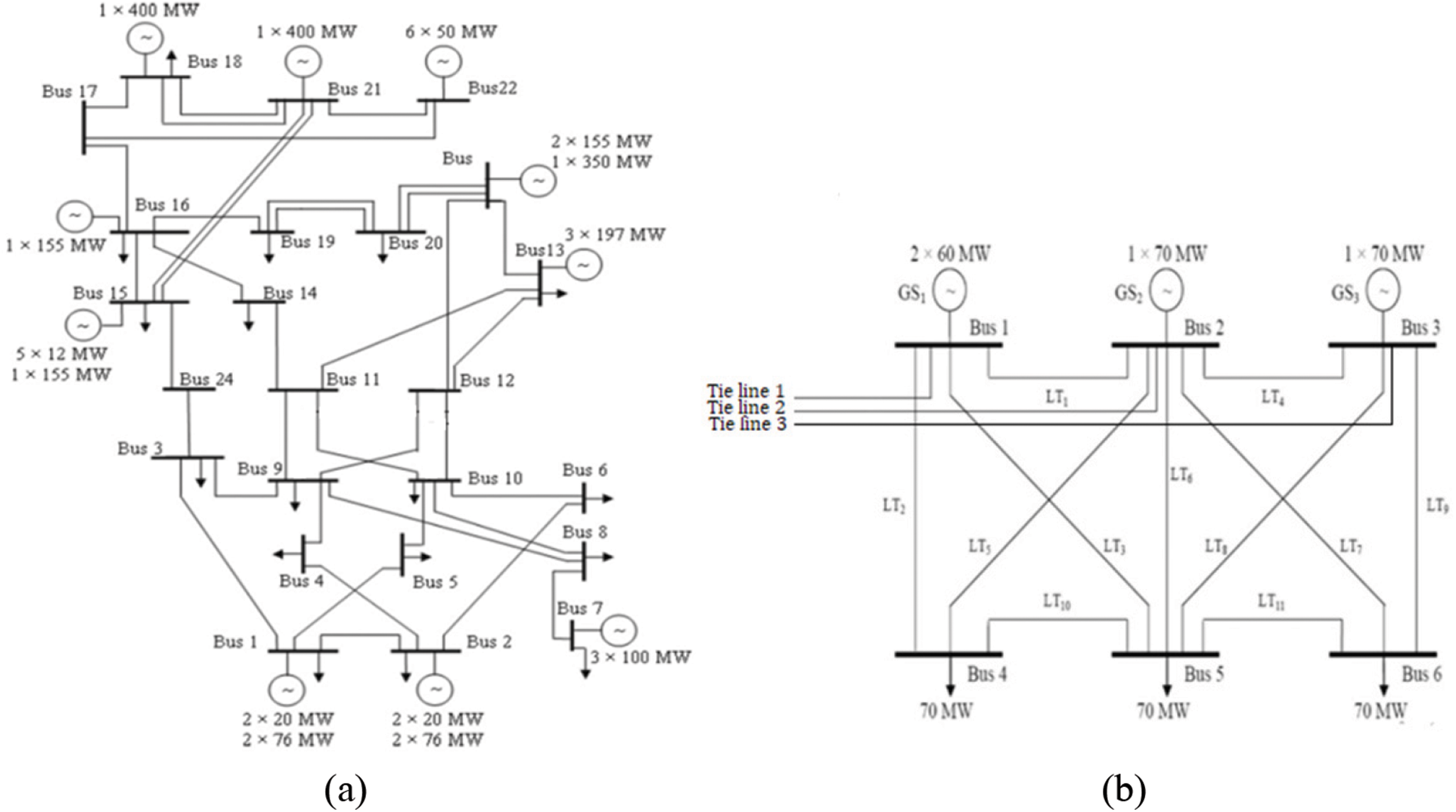
Figure 2: (a) IEEERTS 79 bus (b) 6 bus DG system

MSSA is a simulation procedure to consider the time sequence of the test system. This procedure dramatically reflects the randomness and uncertainty of the entire network [25]. According to the failure rate and repair rate of every part of the network, a random sample of each section is achieved, and then the haphazard failure and repair models are framed. So the entire power network’s operational sequence and their faults in the extended partition and the distribution network can be determined. The original status of the power network in each instant of the extended section and the distribution network is checked. Any component failure and its impact on each load section and the whole system will be arbitrated, and the component failure period will be determined. After 1000000 h of simulation, the reliability index of the load and the system can be found with the relevant equations. Finally, the calculation results of the Reliability assessment of the test system meet the requirement, and the simulation is the end.

The test system is modeled as a composite system designed with the help of MATPOWER tool, which includes the generation and transmission section. The composite section and distribution section are connected through the substation as a low voltage busbar. From the low voltage bus bar side, feeders are extended to connect the IEEE 6 bus system. From the original test system, IEEERTS 79 bus is now extended with IEEE 6 bus system; therefore, the size and level of complexity are increased. In this situation, the reliability assessment of a modified power network is calculated for with and without distributed generating units. After extending the system, the probability of every layer and the capacity is framed. The potential buses for extended integration can be identified using the least sensitivity factor (LSF).

Firstly, every component of the power network is sampled. Assuming the load demand (X) of the respective test system is the expected value (E(ζ)) of a haphazard variable (ζ). The number of sampling is carried out to confer the probability distribution function (ζ). The arithmetic mean value of the distribution function is expressed as,

ζ¯=1Nk∑i=1Nk⁡ζi (15)

when the value of (Nk) is the maximum number, it can get by the following expression.

P(limNk→∝⁡ζ¯=X)=1 (16)

Due to the law of large numbers, we can prove that ζ¯=E(ζ)=X . So, ζ¯ is used for an estimated value of (X). In the test system, the probability of each state is represented as P1, P2, P3 ….., PNk, and its respective frequency is represented as f1, f2, f3 ….., fNk. The time duration and capacity state can be obtained using the statistical method. The probability and the frequency of the (Z) states are expressed as,

Pz=TzTfor,Z=2,3,…,Nk (17)

fz=8760∗IzTfor,Z=2,3,…,Nk (18)

where T is the total simulation time.

Pz is the probability state of Z.

Tz is the time duration of state Z.

fz is the frequency state of Z.

Iz is the occurrence amount of state Z

In the sampling, the computer generates the haphazard number order and can’t be distributed evenly, so the dual sampling method is used to produce a negative association with each haphazard number as the succeeding sampling value to achieve a more accurate value. Let F(Z) be a test of the state z, the probable importance of the test results are as follows:

F(Z)=∑z∈Nk⁡F(z)Pz (19)

F^(Z)=1Nk∑i=1Nk⁡F(zi) (20)

where Nk represents the number of sampling represent the state value of (i) times.

F(zi) is the test results of zi .

F(Z) is an estimated value of F^(Z) .

The distribution section includes the main and lateral line section, distributed transformers, isolators, fuses, breakers with relay, and alternate power supplies (distributed generating units). Here line section and transformers can generally be represented by a 2-state model that is shown in Fig. 3. Here, the upstate represents that components are in the operating condition/state, and the downstate represents that components are not in operation due to failure.

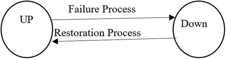
Figure 3: State-space diagram of component

The period when the component remains in the UP state is the Time to Failure (TTF) rate. The time, when the component remains in a downstate is the Time to Repair (TTR) rate. The transition process from upstate to downstate is the failure process, and the down state to up state is the Restoration process. These TTR and TTF are the random variables which are different probability distributions of parameters. The basic three load point reliability indices are average failure rate (λ), average outage period (r), and average annual unavailability or average annual outage time (U).

λi=Ni∑⁡Tui (21)

ri=∑⁡TdiNi (22)

Ui=∑⁡Tdi∑⁡Tui+∑⁡Tdi (23)

where ∑⁡Tui is Summation of all up state times Tu.

∑⁡Tdi is Summation of all the down state time Td.

Ni is the number of failures during the entire sampled year.

The reliability index such as System Average Interruption Frequency Index (SAIFI), System Average Interruption Duration Index (SAIDI), Customer Average Interruption Duration Index (CAIDI), Average Service Availability Index (ASAI), Average Service Un-served Index (ASUI), Expected Un-served Energy (EUE) and Average Expected Un-served Energy (AEUE) of the load and the system could be obtained.

2.5 Integrate Reliability Assessment of the Proposed Test System

The elementary reliability indices at a load point are calculated with the help of three parameters, namely average failure rate ( λi) , average outage time duration ( ri) and average annual outage time durations (Ui) . The integrated calculation of the composite and distribution section of the test system and its reliability indices can be computed using the following equations,

System Average Interruption Frequency Index (SAIFI)

SAIFI=FX=FC+FdX (24)

FC=fz∗Lc (25)

Fd=SAIFId∗X (26)

System Average Interruption Duration Index (SAIDI)

SAIDI=TX=TC+TdX (27)

TC=Tz∗Lc (28)

Td=SAIDId∗X (29)

Customer Average Interruption Duration Index (CAIDI)

CAIDI=SAIDISAIFI (30)

Average Service Availability Index (ASAI)

ASAI=8760∗X−(TC+Td)8760∗X (31)

Average Service Unavailability Index (ASUI)

ASUI=1−ASAI (32)

Expected Unserved Energy (EUE)

EUE=∑⁡LiUi (33)

Average Expected Unserved Energy (AEUE)

AEUE=∑⁡LiUiX (34)

where F is the customer load total interruption time duration in a year

X is the number of customers of a load point

FC is the upper grid (Composite section) side influence on the F

Fd is the lower grid (Distribution section) side influence on the F

T is the total time duration of customer interruption.

TC is the upper grid (Composite section) side influence on the T

Td is the lower grid (Distribution section) side influence on the T

Ui is the annual outage time duration

Li is the average load connected to load point

Lc is the total amount of interrupted customer

SAIFId is the System Average Interruption Frequency Index in the distribution section

SAIDId is the System Average Interruption Duration Index in the distribution section

fz is the frequency state of Z.

Tz is the time duration of state Z.

Here, SAIFId and SAIDId are the distributed side reliability indices, and these indices are not influenced from the composite section of the power network.

3  Results and Discussions

The effectiveness of the developed model is evaluated using IEEE RTS79 [26] integrated with IEEE 6 bus test system, which has the distribution generations in three buses, i.e., PV, WT, and GT at bus number 1′, 2′ and 3′ respectively. The case simulation study is performed using the MATPOWER tool and Modified Salp Swarm Algorithm on a MATLAB platform. The extended six bus system can be integrated with IEEE RTS 79 system in notably through sensitive nodes. Therefore, sensitive nodes for integration are evaluated using LSF and are buses 9 and 10. It is assumed that the capacity of the substation buses, i.e., buses 9 and 10 is the summation of the Peak load. The IEEE RTS 79 test system extended with the IEEE 6 bus test system consists of 30 buses, 51 branch circuits, and 36 generating units distributed among the 14 generating stations. The system’s installed capacity is 3735 MW, with the peak load of 3060 MW connected on 20 buses among 30 buses. Also, the node point of bus 9 and bus 10 is connected to a high voltage busbar of the step-down substation of 230 kV/138 kV. Notably, the summation of substation peak load is equal to 370 MW.

Further, the Expected Energy Not Supplied or Expected Unserved Energy (EENS or EUE) is calculated using the Variance coefficient. The time setting interval of the substation at low voltage bus bar maintained up to 5%, and the ranked capacity table comprises 21 statuses. Also, the simulation time for the assessment program is 1000000 h, and the variance coefficient of EENS is 0.0011093. The complete evaluation is carried out using 7 cases as illustrated below,

Case 1: Base case (no tie line with extended DG system)

Case 2: Combination: Tie line 1- bus no 9 and Tie line 2 – bus no 10.

Case 3: Combination: Tie line 1- bus no 9 and Tie line 3 – bus no 10.

Case 4: Combination: Tie line 2- bus no 9 and Tie line 1 – bus no 10.

Case 5: Combination: Tie line 2- bus no 9 and Tie line 3 – bus no 10.

Case 6: Combination: Tie line 3- bus no 9 and Tie line 1 – bus no 10.

Case 7: Combination: Tie line 3- bus no 9 and Tie line 2 – bus no 10.

3.1 Reliability Indices Evaluation

Case 1

In this case, a base case is simulated to identify the reliability indices of the existing system without the penetration of DGs into the system. The overall assessment is evaluated using MATLAB and the pictorial illustration of the results obtained from MATLAB is given in Fig. 4a. Additionally, the values of AUSI and EUE are derived and found to be 0.000765 and 19091.35 respectively.

Case 2

The penetration of DGs, i.e., PV, WT, and GT, is analysed in this case. As stated earlier, the potential location for DG penetrations is computed as bus 9 and bus 10. Therefore, Tie lines 1 and 2 are connected to bus no 9 and bus no 10, respectively. Further, the reliability assessment is carried out using indices after DG penetration, and the detailed values are illustrated in Fig. 4b. The other indices such as AUSI and EUE are found noble: 0.000798 and 21382.89 respectively. It is perceived that the penetration of DGs enhanced the overall system indices commendably compared with the existing base case, notably on SAIFI, SAIDI, and CAIDI indices. It is due to the fact of the line characteristics which is most optimistic in this case.

Case 3

Similar to case 2, the DGs penetration is performed with two buses. Tie line 1 and Tie line 3 are connected to bus no 9 and bus no 10, respectively. Again, the reliability assessment is carried out using indices, and the detailed scales are represented in Fig. 4c. It is observed that the overall system reliability indices are enhanced noticeably compared to the existing case but not great with case 2.

Case 4

In this case, the penetration of DGs, i.e., Tie line 2 and Tie line 1 are connected to bus no 9 and bus no 10, respectively. The reliability assessment indices display improved value compared with the existing system and case 3 but show less performance than case 2, as illustrated in Fig. 4d.

Case 5

The integration of DGs is performed using the same nodes as mentioned in previous cases but using different Tie lines, i.e., Tie line 2 and Tie line 3 are connected to bus no 9 and bus no 10, respectively. Owing to the indirect penetration of higher capacity through Tie line 2 and Tie line 3, the reliability assessment indices display some declined values compared with other cases discussed above except base system, as illustrated in Fig. 4e.

Case 6

This case analyzed the indices, similar configuration of case 3 but with interchanged Tie line connection. While comparing the observed results, it is found that the system indices are significantly greater than case 3, case 4, and case 5, but closer results with case 2: nonetheless, not higher than case 6 (Fig. 4f).

Case 7

In this case, Tie line 3 and Tie line 2 are connected with bus 9 and bus 10, respectively, replicating the configuration of case 5 but with interchanged tie line arrangements. Comparing with base system and case 5, this configuration shows improved indices, but not great with other cases, as illustrated in Fig. 4g.

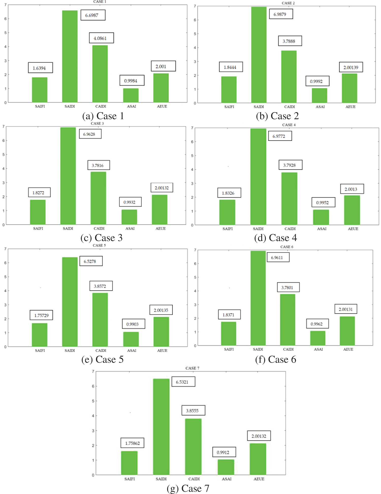
Figure 4: System indices for all the seven cases

3.2 Available Capacity on the Low Voltage Bus Side

The assessment of hierarchical capacity on low voltage bus bar can attain the same precision to reflect a characteristic of the test system veritably, and the corresponding calculated results are illustrated in Tab. 3. From the Table, the status probability shows that the available capacity at bus 9 and bus 10 (Case 2) is equal to 370MW, which is greater than 80%. Therefore, most of the time duration, the consumer load is met with sufficient capacity. In addition, the probability of every status decrease monotonically with the same degree of available capacity reduction is found. Between 185 and 18.5 MW, the probability of the status is zero.

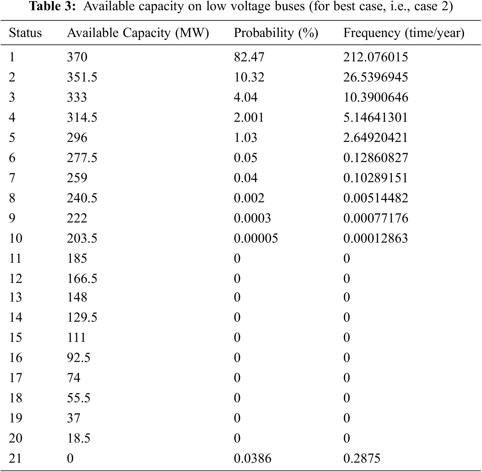
The probability of the 21st status is not zero because the trouble due to un-reasonable maintenance leads to the failure of the substation on the low voltage bus bar section.

4  Comparative Analyses

A detailed comparative study between all the cases is performed and illustrated in Fig. 5. Fig. 5a shows that the reliability indices SAIFI attained a percentage improvement of about 12.50% for case 2, which is commendably great compared with the existing system. It is owing to the penetration of higher DGs capacities through tie lines. Further, the indices SAIDI maintained a 4.32% improved value for case 2 compared with other cases, as described in Fig. 5b.

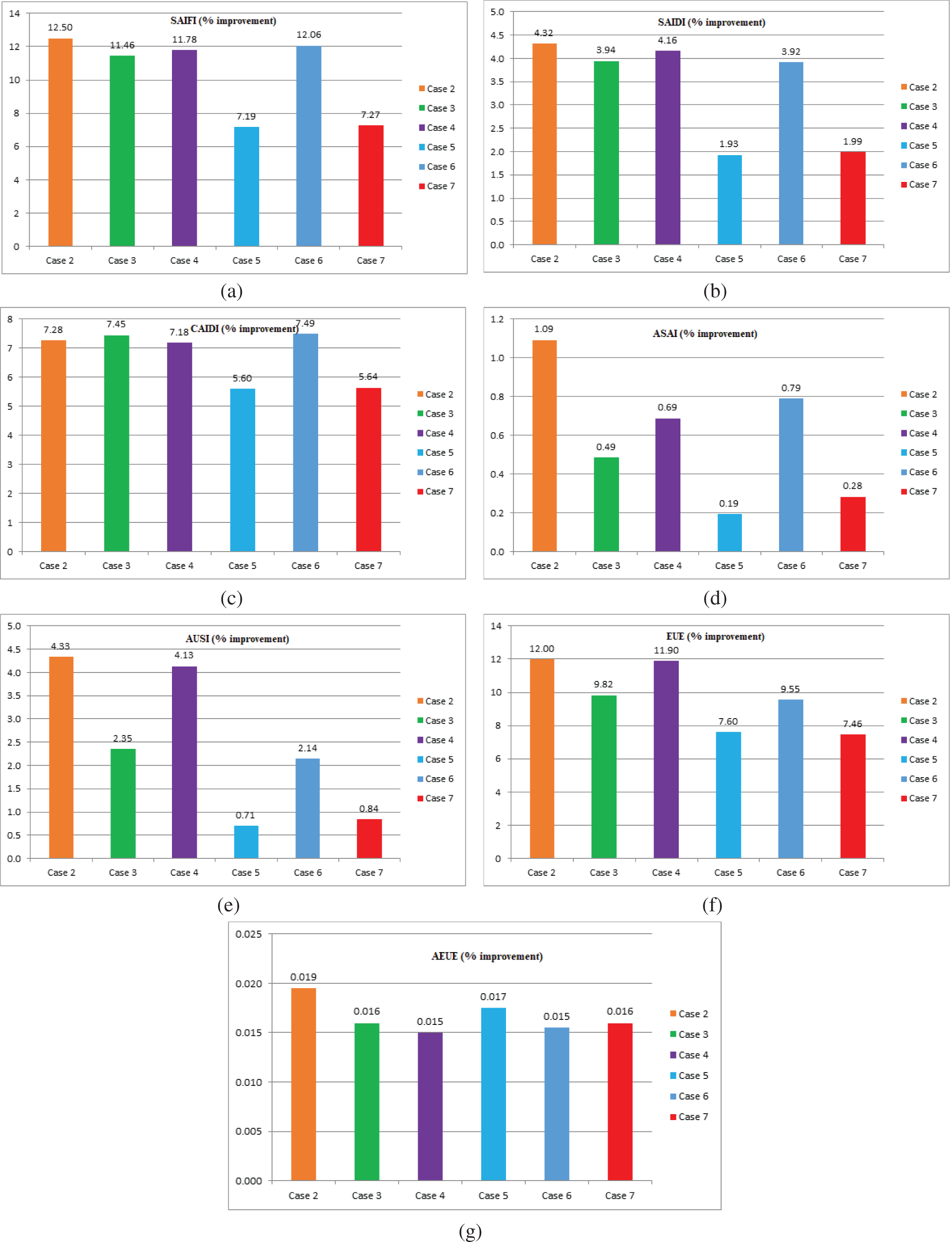
Figure 5: Percentage improvement of systems reliability indices (a) SAIFI (b) SAIDI (c) CAIDI (d) ASAI (e) AUSI (f) EUE (g) AEUE

Similarly, the other indices such as CAIDI, ASAI, AUSI, EUE, and AEUE display a superior enhancement scale of about 7.28%, 1.09%, 4.53%, 12.00%, and 0.19%, respectively for case 2, as illustrated in Figs. 5c–5g. Considering all these inferences from the observed outcomes, it is perceived that the case 2 configuration significantly enhances the existing system after DGs penetration through the tie lines.

Further, the effectiveness of the MSSA is compared with the conventional SSA for the best case attained in this work. It is noted that the proposed modifications in the MSSA helps to obtain better a reliability of the considered system using evaluation indices (Fig. 6). MSSA effectively improves the exploration ability of original SSA by modifying the constant value of k1 as 0.1, and avoids the local optima. Modified SSA technique reduces the execution time compared with SSA technique, in turn improves the exploitation ability of the algorithm.

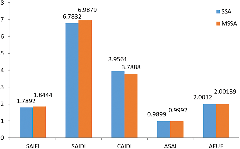
Figure 6: Comparison of MSSA with SSA

In a nutshell, the meta-heuristic algorithm effectively evaluates the reliability indices for all the considered cases that comprise different DGs penetration schemes through available tie-line possibilities. Also, the total run time of the algorithm is small, about 4.01 s for the existing case, and 5.02 s for integrated configurations, i.e., after DGs penetration. Also, run time of the system depends on system configuration and optimization level, it can be reduced by altering the weightage of the parameters. Consequently, this algorithm can be adapted for a large-scale system that could generate commendable results.

5  Conclusions

A reliability assessment and available capacity of extended system is studied in this work using modified salp swarm algorithm (MSSA). The wok procedure and their simulation results display some notable effects, as described follows: The proposed MSSA algorithm facilitated to assess the distribution section’s reliability indices considering the influence DGs penetration with existing system. There were seven different configurations considered to assess the superior Tie-line integration. Among these, case 2 that connects the Tie line 1 and Tie line 2 with bus 9 and bus 10, respectively displayed superior results in terms of indices and availability capacity. Further, the reliability indices of best case such as SAIFI, SAIDI, CAIDI, ASAI, AUSI, EUE, and AEUE exhibited better enhancement about 12.5%, 4.32%, 7.28%, 1.09%, 4.53%, 12.00%, and 0.19%, respectively. Also, the probable availability capacity at the low voltage bus side was found to be 82.47%. Furthermore, the frequency of the availability was measured to be 212.07 times/year. The total computation time of the algorithm was found to be small about 5.02 s after DGs penetration.

The above results warrant the effectiveness of the proposed meta-heuristic algorithm for extended system particularly for DGs integration. This proposed scheme can be adapted for any standard or real-time system, comprises large system dimensions. However, the computation time of the algorithm may increase accordingly that may cause a complexity in the computation process and this can be addressed in the future works.

Funding Statement: The authors received no specific funding for this study.

Conflicts of Interest: The authors declare that they have no conflicts of interest to report regarding the present study.

This work is licensed under a Creative Commons Attribution 4.0 International License, which permits unrestricted use, distribution, and reproduction in any medium, provided the original work is properly cited.