Computer Systems Science & Engineering DOI:10.32604/csse.2023.027239
Article

Time Delay Estimation in Radar System using Fuzzy Based Iterative Unscented Kalman Filter

T. Jagadesh1,2 and B. Sheela Rani3,*

1Faculty of Electronics Engineering, Sathyabama Institute of Science and Technology, Chennai, 600119, India
2Department of ECE, KPR Institute of Engineering and Technology, Coimbatore, 641407, India
3Sathyabama Institute of Science and Technology, Chennai, 600119, India
*Corresponding Author: B. Sheela Rani. Email: kavisheela66@gmail.com
Received: 13 January 2022; Accepted: 06 April 2022

Abstract: RSs (Radar Systems) identify and trace targets and are commonly employed in applications like air traffic control and remote sensing. They are necessary for monitoring precise target trajectories. Estimations of RSs are non-linear as the parameters TDEs (time delay Estimations) and Doppler shifts are computed on receipt of echoes where EKFs (Extended Kalman Filters) and UKFs (Unscented Kalman Filters) have not been examined for computations. RSs, certain times result in poor accuracies and SNRs (low signal to noise ratios) especially, while encountering complicated environments. This work proposes IUKFs (Iterated UKFs) to track online filter performances while using optimization techniques to enhance outcomes. The use of cost functions can assist state corrections while lowering costs. A new parameter is optimized using MCEHOs (Mutation Chaotic Elephant Herding Optimizations) by linearly approximating system non-linearity where OIUKFs (Optimized Iterative UKFs) predict a target's unknown parameters. To obtain optimal solutions theoretically, OIUKFs take less iteration, resulting in shorter execution times. The proposed OIUKFs provide numerical approximations which are derivative-free implementations. Simulation evaluation results with estimators show better performances in terms of reduced NMSEs (Normalized Mean Square Errors), RMSEs (Root Mean Squared Errors), SNRs, variances, and better accuracies than current approaches.

Keywords: Radar system; unscented kalman filter; extended kalman filter; optimized iterative unscented kalman filter; mutation chaotic elephant herding optimization; time delay estimation

1  Introduction

Target identifications/tracking, management of air traffic, and remote sensing are all common use of RSs [1,2] where transmitters send signal bursts, and receivers receive dispersed versions of those signals. The scattering of signals is measured using TDEs and Doppler shifts in received signals and the target’s range and radial velocities are computed. These measurements are employed as measurements in RSs [3]. The fundamental concept of Radars is similar to that of sound wave reflection. Radars detect and locate objects by using electromagnetic radiation bursts. Radars can be classified in a variety of ways but categorized into eleven groups based on their functionality and primary characteristics [4].

Generic pulse Radars play a prominent role in RSs where they emit a series of short-duration rectangular pulses in repeated patterns. Pulse Radars can be divided into two categories namely Radars with MTYIs (Moving Target Indications) and Radars with pulse-doppler. Both these types employ Doppler frequency shift, which works with incoming signals to find a moving target. The TDEs and Doppler shift are used to calculate measures like range and radial velocity based on these two kinds. Difficulties in calculating TDEs between received signals of the same transmitters are known as TDEs [5] where computing these parameters are critical for detecting targets with radar transmitters. These received echoes are referenced with signals by the usage of filters to estimate TDEs and assure target recognitions.

KLMSs (Kernel Least Mean Squares) are new approaches in non-linear estimation [6–8] that efficiently estimate TDEs and Doppler shifts. RKHSs (Reproducing Kernel Hilbert’s Spaces) use representer theorems and estimate nonlinearity between unknown parameters iteratively while returning signals using KLMSs estimators. The LMS method in RKHSs adaptively updates calculated parameters.

EKFs and UKFs are commonly used nonlinear estimators and have been evaluated for tracking targets in radar measurements [9,10]. Certain specific applications of synthetic aperture radars, Kalman filter’s version MCKFs (Modified Convolution Kernel Functions) [11] estimated parameters of returning LFMSs (Linear Frequency Modulated Signals). EKFs and UKFs have not been examined to estimate the TDEs and Doppler shifts in target tracking applications.

However, they approximate nonlinear systems with first-order linearization to produce linear models. In complicated environments with low SNRs and heavy-tailed clutter, they have poor accuracies and stability resulting in ambiguous Target identifications. Improved EKFs and UKFs evaluate systems with their true nonlinear forms, which helps in accurate parameter estimates even in a complicated context. However, the purpose of IEKFs is to iteratively search for improved linearization that is suited for severe nonlinearities, rather than to directly correct linearization mistakes. IEKFs are a natural extension of EKFs that combine NLSs (Nonlinear Least-Squares) with GNs (Gaussian Newton).

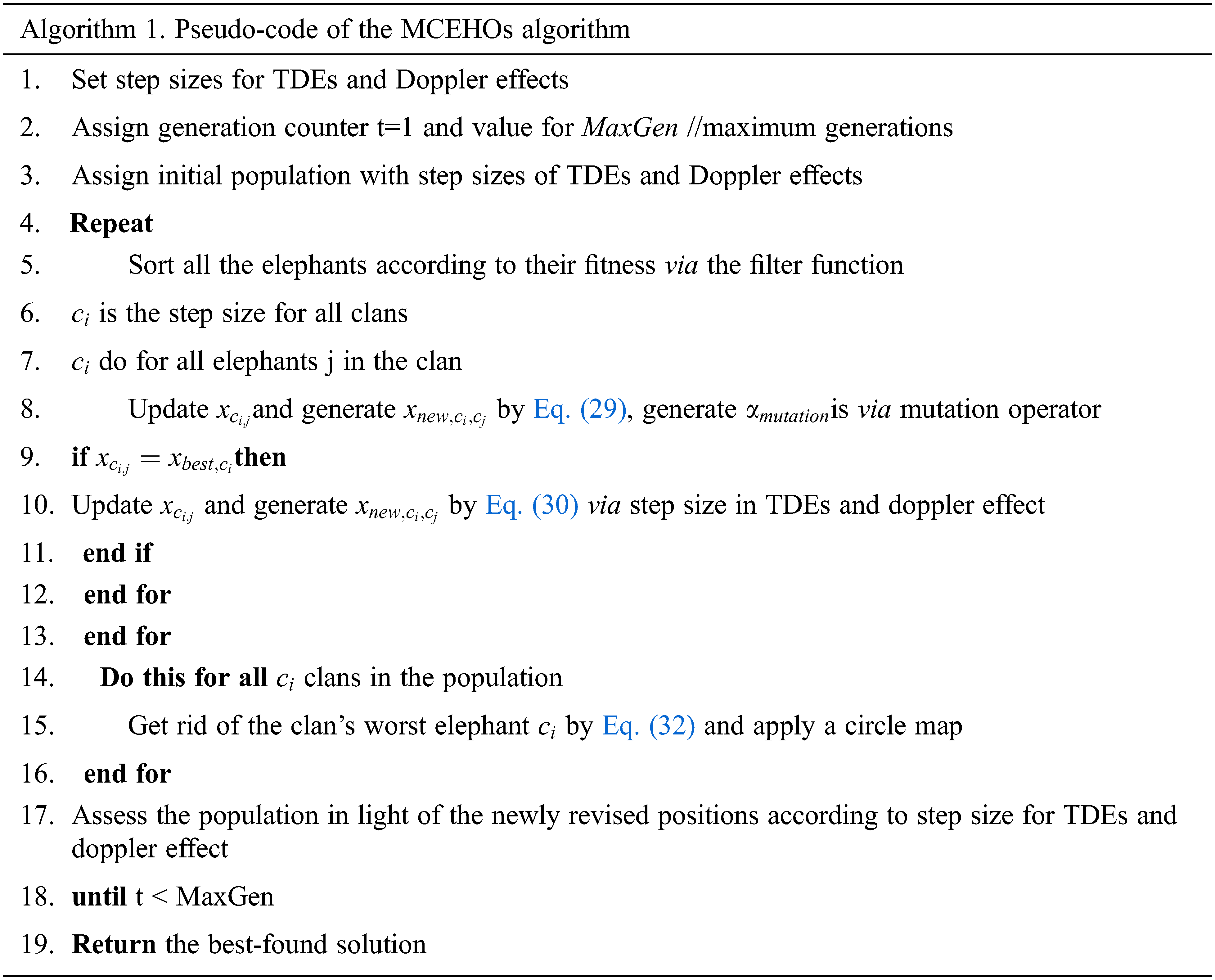
This study proposes OIUKFs for monitoring filter performances online and attempting to improve them using optimization techniques. The use of cost functions can monitor state corrections and lower costs. A new parameter is optimized using MCEHOs which approximates the system’s nonlinearity and OIUKFs which estimate a target's unknown parameters. The underlying cost functions are optimized using OIUKFs based on MCEHOs approach. This study achieves enhanced accuracies as demonstrated in its simulation results.

2  Literature Review

Singh et al. in their study proposed non-linear estimations based on sparse KLMSs (Kernel Least Mean Squares). Their scheme used adaptive kernel width optimizations for reducing computational complexities and easier implementations. The study used modulated and orthogonal frequency divisions multiplexed Radar signals where Cramer-Rao lower bounds were constructed for their proposed estimations. Target ranges were estimated by Singh et al. where unique iterative non-linear KLMSs estimations were used. Their scheme when compared with FTs (Fourier Transforms) based estimation in simulations showed KLMSs converged with reduced MSEs. KLMSs have significant limitations in assessments on characteristics including kernel widths, step sizes, and dictionary threshold values, and when these parameters are run on specified ranges, they yield suitable values.

Kulikov and Kulikova suggested Accurate Continuous-Discrete EKFs based on ODEs (Ordinary Differential Equations) with global error controls. They compared their proposed scheme with Continuous-Discrete Cubature and UKFs using seven-dimensional radar tracking where airplanes made coordinated turns. The study proved the worthiness of nonlinear filtering techniques in their tests by using them for actual target tracking however, their Accurate Continuous-Discrete EKFs were found to be versatile and resilient in their tests. It could successfully address air traffic control situations for diverse data and a variety of sample times without any manual adjustments.

Gu et al. suggested multi-component LFMSs parameter estimations based on MCKFs. The suggested scheme was quicker as there were no searching operations, reducing external influences, and lowering computing burdens. Furthermore, it was resistant to additive noises. Their suggested strategy was supported by simulated and real-world data. On the other hand, EKFs and UKFs have not been used to estimate the TDEs and Doppler shift for target tracking.

For global optimization issues, Ibrahim et al. [12] presented SKFs (Simulated Kalman Filters), population-based meta-heuristic optimizations based on Kalman Filter estimations. State estimations were treated as optimization issues where SKF agents were Kalman Filters. Nonlinear estimators based on KLMSs were proposed by Singh et al. [13] and they outperformed traditional estimators. KLMSs estimators have poor selections of system parameters and to overcome their limitations nonlinear estimators namely EKFs and UKFs were used in this study. EKFs were selected due to their ease in implementations, but suffered from inadequate representations of nonlinear functions for 1st order linearization, while UKFs outperformed EKFs by providing stableness by treating nonlinearities precisely. The suggested EKFs and UKFs-based estimators of the study enhanced accuracies, according to the study’s simulation findings.

Mishra et al. [14] investigated sub-Nyquist cognitive radars in which overall transmitting powers of multi-band cognitive waveforms were conventional equivalent to full-bands which lowered MSEs of single-target TDE estimates. To improve the accuracies of delay estimations, the study selected the best bands and distributed total power in the bands. Using Cramer-Rao limits, the study showed that in cognitive radars, equal width sub-bands resulted in superior delay estimations than conventional radars. Cognitive radar performed effectively in terms of low SNRs in their investigation utilizing Ziv-Zakai bounds.

Roemer et al. [15] examined the challenge in predicting unknown delay(s) as systems receive linear combinations of multiple delayed copies of known broadcast waveforms. This issue was noticed in a variety of applications, including timing-based localizations and wireless synchronizations. To reduce hardware complexities, the study suggested a compressed sensing-based system design that measured values below Nyquist rates, and yet delay estimates were accurate. The study’s design of kernels for measurements with frequencies showed optimal numerical choices and outperformed functions that were randomly chosen for estimating delays.

Cobos et al. [16] suggested a sub-band technique for the estimation of TDEs to increase traditional GCC (Generalized Cross-Correlation) algorithms. Their suggested method used sliding windows to extract numerous distinct correlations amongst the cross-power spectrum’s frequency bands of the phase. Their key contributions could be summed up as 1) GCC sub-band representations of cross power spectrums which have lower temporal resolutions and estimate TDOAs (Time Difference of Arrival) 2) When signals are without noises their matrix representations exploited scenarios for achieving robust and accurate GCCs; 3) designing low-rank approximations for processing GCC sub-band matrices resulting in improved TDOA estimates and source localization performances. To show the validity of their suggested technique, their scheme was tested with a large number of experiments.

Li et al. [17] introduced a new approach for exploiting space-frequency features to estimate DOAs (Direction-of-Arrivals) and TDEs of multi-path OFDM (Orthogonal Frequency Division Multiplexing) signals. The study’s scheme combined array structures and frequencies to generate extended virtual arrays. The study reduced impacts of multi-path by constructing extended channel frequency response matrices which were smoothened.

Compressed Sensing which reach high resolutions were exploited by Li et al. [18] to estimate signal parameters based on the signal’s sparseness. Their approaches used high resolutions after l0-norm Optimizations. Generalized filter outputs or ambiguous functions result in sparse representations where prior studies used sparse representations for channel responses. The study deconvolved outputs of generalized matching filters using greedy optimizations and bayesian methods for two-dimensional estimations of Doppler shift and TDEs. Their simulations showed that their technique outperformed other sparse representations of channel data in low SNRs.

3  Proposed Methodology

The main aim of this study is to predict TDEs and Doppler shifts (radial velocities) of signals. These estimations are based on non-linear estimation approaches namely OIUKFs and EKFs. To obtain theoretical optimal solutions, OIUKFs consume less iteration, resulting in shorter running times, and are useful for estimating the target’s properties accurately even in complicated contexts. This study’s suggested estimators showed lower errors and variances in simulations.

3.1 Signal Model Formulation

This section derives radar return signals by connecting radar return and required unknown parameters like TDEs and Doppler shift where mono-static LFM radars [3] were used to keep radars static. Radar’s transmitters emit LFM pulses at baseband frequencies with LFM pulses separated by set periods called PRIs (Pulse Repetition Intervals). Received signals get dispersed from their initial broadcasting signals. This scattering occurs due to two factors namely TDEs (signal transmissions between antennas and targets and Doppler shifts which occur due to radial velocities of targets.

The LFMSs (vLFM(t)) can be depicted as in Eq. (1)

vLFM(t)={aexp⁡(jπγt2);0≤t≤To0;T0<t<TPRI (1)

where, a - amplitude, γ - sweep rate’s frequency, To - duration of pulses, and TPRI - PRIs. The frequency of LFMSs varies with time where the immediate frequency is computed using fi(t)2=γt . mth pulse when MLFM pulses burst can be represented as time-shift forms of LFMSs and shown in Eq. (2),

vj(t)=v(t−nTPRI)for0≤t≤To (2)

where, n∈[0,1,...,N−1] and N represents total pulses count in a burst. vj(t) gets modulated by high-frequency carrier signals where modulations can be represented mathematically as Eq. (3),

v(t)={vj(t)}exp⁡(j2πfct) (3)

where, fc -carrier signal’s frequency. Returning signals pm(t) are time delayed variants of v(t) where τm stands for TDEs of the mth pulse when Eq. (4) is satisfied,

τm=τo−2C{vmTPRI} (4)

where τo -first pulse’s TDE, v - radial velocity, and c – light’s velocity. For maintaining generality of target’s time (N pulses) v is considered constant or constant Doppler shifts are assumed. Then Time differences 2/c { vm TPRI} in time shifts of return signals when targets change positions over nTPRI results in subsequent changes to pn(t) and given by Eq. (5),

pn(t)={vj(t−τn)}exp⁡(j2πfc(t−τn))+km(t) (5)

where, km(t) - additive thermal noises Returning signals, pn(t) , of basebands when depicted mathematically, form Eq. (6),

pm(t)={vj(t−τn)}exp⁡(−j2πfcτn)+km(t) (6)

This implies Pn(f) can be written as Eq. (7),

Pn(f)=|VLFM(f)|2exp⁡(−j2πfcτn)exp⁡(−j2πfτn)+km(f) (7)

Where, VLFM(f) represents Fourier transforms LFMSs Sampling frequency l=[0,1,..,L−1] with interval Δf and dividing by |VLFM(lΔf)|2 yields the following Equation

p(n,l)=exp⁡(−j2πfcτn)exp⁡(−j2πΔfτn)+k(n,l) (8)

where k(n, l) represents thermal noise’s discrete samples. Substituting τn from Eq. (4) results in Eq. (9),

p(n,l)=exp⁡(j2πnfdTPRI)exp⁡(−j2πlΔfτo)exp⁡(j2πfdml(TPRIΔffc))+k(n,l) (9)

Where fc= 2vfc/c represents unknown Doppler shifts caused by the target’s radial velocities. From Eq. (9), it can be noted that returning signals, r(m, l), are nonlinearly and exponentially related to TDEs ( τo and fd ) which are estimated from returning signals r(m, l) using EKFs and UKFs. Gaussian filters were used instead of particle filters as result in acceptable estimation with low processing costs. The suggested EKFs and OIUKFs for estimating TDEs are Gaussian filters. The LFM radar system’s states assessment model was developed using the Bayesian framework followed by EKFs and OIUKF estimations for τo and fd .

This study uses notations for mathematical representations where constants are in upper cases, Vectors are boldfaced upper cases, superscript representations are: ( T transposes. H complex conjugate transposes of matrices and * scalar complex conjugate operations), statistical expected outcomes are represented by E[⋅] . R denotes real numbers while C stands for complex numbers where R (·) implies real parts and I (·) stands for imaginary parts.

3.2 States Assessment Models for RSs

This work’s proposed state assessments include measurements models where the states are measured using mathematical links. TDEs ( τo and fd ) form the state, while the observed values (returning signals p(n,l)) constitute measurements and variables declared included x=[τofd]T and y=[R(r(m,l))I(r(m,l))]T . The state-space model defined in Eq. (9) rise consistently in intervals and TDEs due to the assumed constancy of radial velocities. Errors arising from this study’s assumptions of constants are treated as process noises. The modeled state can be depicted mathematically as Eq. (10),

yk+1=f(yk)+ηk = yk + Δy + ηk (10)

where k∈{1,2,…,K} , K=ML stands for discretized sample counts of signals returned, and Δx=[ToK,0] represents shifts between successive returning signals. ηk is the noise that are additive and assist in modeling error compensations. Based on Eq. (9), measurements ( xk+1 ) can be depicted as Eq. (11),

xk+1=c(xk+1)+dk+1=[R(exp⁡(j2πnyk+1(2)TPRI)exp⁡(−j2πlΔfyk+1(1))exp⁡(j2πyk+1(2)ml(TPRIΔffc)))I(exp⁡(j2πnyk+1(2)TPRI)exp⁡(−j2πlΔfyk+1(1))exp⁡(j2πyk+1(2)ml(TPRIΔffc)))]+vk+1 (11)

where dk stands for noises measured. These measurements help mitigate signal errors that occur while collecting/processing them. ηk , vk represent Gaussian filter’s assumed zero means with covariance Qk and Rk. This study considers the additive impacts of process/measurement noises.

3.3 Bayesian Filters

Bayesian filtering is a two-step operation using predictions and updates:

3.3.1 Predictions

This phase creates the PDFs (Probability Distribution Functions) of states one-time step forward (relation to the available observations) by utilizing Chapman–Kolmogorov equation [19] given as Eq. (12),

P(yk|x1:k−1)=∫P(yk|yk−1)P(yk|x1:k−1)dyk−1 (12)

where P(·) stands for PDFs and P(yk|x1:k−1) stands for prior PDFs.

3.3.2 Update

PDFs are reconstructed in this step when new measurement values from Bayes rule [19] yk are received and depicted as Eq. (13),

P(xk|y1:k−1)=P(xk|y1:k−1,yk)=1/ckP(yk|xk)P(xk|y1:k−1) (13)

ck=P(yk|y1:k−1)=∫P(yk|xk)P(xk|y1:k−1)dxk (14)

where P(yk|xk) stands for likely measures achieved using Eq. (11) and ck represents constant for normalizations. The use of Bayesian filtering results in the construction of posterior PDFs P(xk|y1:k).

3.4 TDE Estimations Using EKFs

The estimations of TDEs ( τo and fd ) from returning signals, r(m, l) of the investigated RSs using Eqs (10) and (11) are simplified from states assessment as estimations of x k from known y k measurements where EKFs are analytical simplifications of Bayesian frameworks and where conditional PDFs in Bayesian frameworks Eqs. (12)–(14) are assumed to be Gaussians as shown in Eq. (15),

P(xk|k−1)∼N(xk|k−1;x^k|k−1,Pk|k−1) (15)

P(xk|k)∼N(xk|k;x^k|k,Pk|k) (16)

where, real Gaussian distributions are represented as N, xk|k−1 stands for mean values while Pk|k−1 implies covariance of xk|k−1 and similarly xk|k implies mean values and Pk|k covariance of xk|k . xk|k−1 and Pk|k−1 are predicted while xk|k and Pk|k are updated as detailed below:

3.4.1 Prediction

In this step, prior PDFs ( xk|k−1 and Pk|k−1 ) result when Jacobian (Fk) of f(xk) [19] is used and depicted as Eq. (17),

Fk=∂f(x)∂x|x= x^k−1|k−1=[1001] (17)

3.4.2 Update

In the initial part of this step, measurements (y^k|k−1) are predicted along with error covariance ( Pk|k−1YY ) using Jacobian (Hk) of h(·) [19] which results in new measurements yk . Subsequently, posterior estimates and covariances, x^k|k−1 , and Pk|k , are obtained using Kalman filter gains ( Kk ) where posterior estimations x^k|k=[τ^okf^dk]T results desired TDEs and Doppler shift outcomes.

3.5 Optimized Iterative Unscented Kalman Filter (OIUKF)

The calculation of an IUKF using the Fisher estimation framework is described in [20], and it entails minimizing the following cost function in the filter’s measurement update phase.,

y^t|t=argminy⁡Z(y)=argminy⁡12fT(y)f(y) (18)

f(y)=[Rt−12(yt−h(x))Pt|t−1−12(x^t|t−1−x)] (19)

Hi=(Pixy)TP−1 (20)

It presupposes, like the IUKF version, that the measurement function is affine in the vicinity of x and x i, and therefore that h x' (x)=h x' (x i)= H i. The Jacobian H i is not explicitly computed in the UKFs, but the fact that Pxy = PHT in the linear case may be used to infer a stochastic linearization. As a result, the equation provides a fair estimate of H i in the IUKF (20),

When P’s symmetry has been exploited and Pxy implicitly incorporates second-order transformation effects [21]. The state iteration in IUKF may be utilized to generate the following equation using the preceding stochastic linearization approach (21),

xi+1=x^+Ki(y−y^i−(Pixy)TP−1(x^−xi)) (21)

Ki=Pixy(Piyy)−1 (22)

y^i=∑kW(k)Yi(k) (23)

It can be utilized as a starting point in the IUKF It’s worth noting that y = y (t|t − 1) remains constant. The projected measurement y i must still be determined. The equation can be used to express two different natural alternatives (23),

y^i∗=Yi(0) (24)

i.e., the converted center sigma point, represented by the superscript * in this case. Two somewhat different interpretations of the cost function by equation result from the two options (25),(26).

V(x)=(yt−E[h(x)])TRt−1(yt−E[h(x)])+(x^t|t−1−x)TP(t|t−1)−1(x^t|t−1−x) (25)

V∗(x)=(yt−h(x))TRt−1(yt−h(x))+(x^t|t−1−x)TP(t|t−1)−1(x^t|t−1−x) (26)

both depict different approximations of costs where corrections to states can result in decreased costs i.e., V(xi+1)<V(xi) . If this is not the case a step size parameter α by Eq. (27).

yj+1=yj+αj(y^−yj+Gj(x−x^j−Hi(x^−xi))) (27)

MCEHOs are used to compute the step sizes where EHOs (Elephant Herding Optimizations) use both global and local searches [22]. Local searches, on the other hand, aim to locate better step sizes in smaller search spaces with smaller promising approximate predictions of time and Doppler flaws. Elephant’s herding behaviors are characterized as elephant populations (with varying step sizes) split into clans. Generations have males which leave their clans for optimal selections of step sizes. Clans represent local searches in the algorithm through the optimum selection of step sizes, but male elephants leaving clans are global search implementations through step sizes. Matriarchs are solutions (elephants) in the clan with the best fitness values for TDEs. Moving male elephants, on the other hand, are solutions τo and fd with the worst fitness function of RSs. MCEHOs approach divides Elephant population into k clans which are D-dimensional solutions created randomly in search spaces by using lower bounds xmin and upper bounds xmax of TDEs and using Eq. (28),

x=xmin+(xmax−xmin+1)rand (28)

where, rand implies random numbers between (0,1). New solutions get generated in generations when clan members (j) from clan (ci)with best fitness values get attracted by solutions ( xbest,ci ) [22]:

xnew,ci,cj=xci,cj+αmutation(xbest,ci−xci,j)rand (29)

where, xnew,ci,cj - j’s new solution in clan ci for optimal selection of steps size in TDEs and doppler effects, xci,cj - previous generation’s solution, αmutation - generated parameter via mutation operator and algorithm’s parameter is set correspondingly for TDEs and doppler effect. If the mutated value is worse than the new value that is created via the new mutated value. rand∈[0,1] random numbers between (0,1) in uniform distributions. Scaling factor α influences best TDEs and doppler effect values with their step sizes and these positions in clans get updated based on Eq. [22] given below:

xnew,ci=βxcenter,ci (30)

where [0,1] is the second algorithm parameter, which determines the clan center’s effect. xcenter,ci for TDEs and doppler effect. Clan center is defined by Eq. (31) [22],

xcenter,ci,d=1nci∑l=1ncixci,l,d (31)

where 1 ≤ d ≤ D represents the dth dimension and nci is the number of reduced TDEs and doppler effect in clan ci . In each clan, nci solutions with the worst fitness values for TDEs and doppler effect of the clan ci are chosen to be replaced by the following Eq. (32) [23],

xworst,ci=xmin+α(xmax−xmin+1)rand (32)

where xmin and xmax represent lower and upper bounds of search spaces for TDEs and doppler effects in the interval rand ∈ [0,1] TDEs and the doppler effect was used to represent a random integer from uniform distributions where they use two separate one-dimensional maps, circles, and sinusoidal maps, to generate random numbers. The circular maps [23] can be described by Eq. (33),

yg+1=[yg+a−b2πsin⁡(2πyg)]mod1 (33)

where the produced chaotic sequence is inside b = 0.5 and a = 0.2 (0, 1). The equation for a sinusoidal map is (34) [23],

yg+1=byg2sin⁡(πyg) (34)

where for b = 2.3 and y0 = 0.7 the following simplified form.

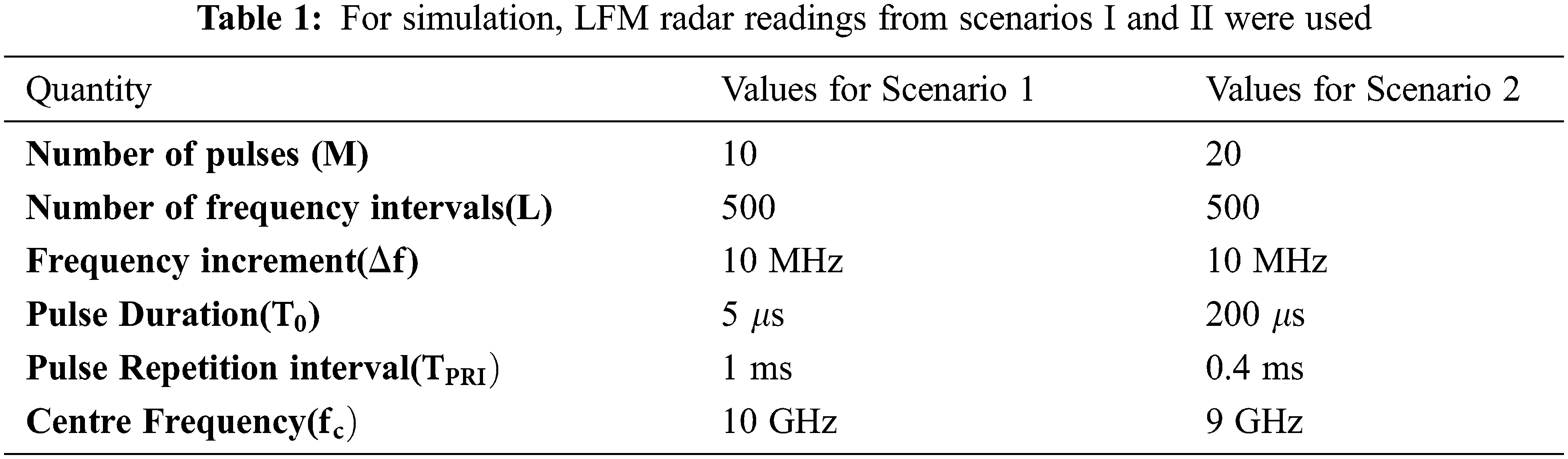
The proposed scheme using EKFs and OIUKF estimations was tested with MATLAB simulations and compared with other non-linear estimators based on UKFs, KLMSs, and Modified NCs. Two mono-static RSs with different parameter values were studied and listed in Tab. 1 for Scenarios 1 and 2 which refer to the two RSs [24]. Scenario 1 depicts realistic LFM RSs where parameter values differ from Scenario 2’s RSs. These scenarios are generated using a radar toolbox in MATLAB.

For both Scenarios 1 and 2 estimators based on EKFs and OIUKFs [25], Rk=σv2I (where σv2 is obtained according to specified SNRs defined as relative strengths of signals with respect to noises in this work

SNR=c(yk+1)Tc(yk+1)/nσv2 (35)

TDEs and Doppler shift were estimated for SNR of 20 dB; however, a comparative study is presented for SNRs ranging from 30 to 20 dB. For UKFs and both Scenarios 1 and 2, =0.5 were evaluated with 5 sigma points in simulations taking 2n +1. (where n is the dimension or 2 in this study) [22].

Fig. 1 shows that EKFs and OIUKF-based estimating procedures achieve the final NMSE around the 3000th iteration, UKFs-based estimation around the 3500th iteration, and KLMS Modified NC around the 4500th iteration. Furthermore, OIUKF achieves a substantially lower final NMSE than the other approaches. As a result, whereas estimators based on EKFs, UKFs and KLMSs Modified NC require longer to converge, the OIUKF-based estimator converges quickly and achieves a substantially lower final MSE than previous approaches. Fig. 1 shows that the proposed OIUKF-based estimation has a lower NMSEs of 0.0032, whereas other approaches such as EKFs, UKFs, and KLMS Modified NC have higher NMSEs of 0.42, 0.029, and 0.012, respectively, for 5000 iterations in scenario 1 in Estimation of TDEs.

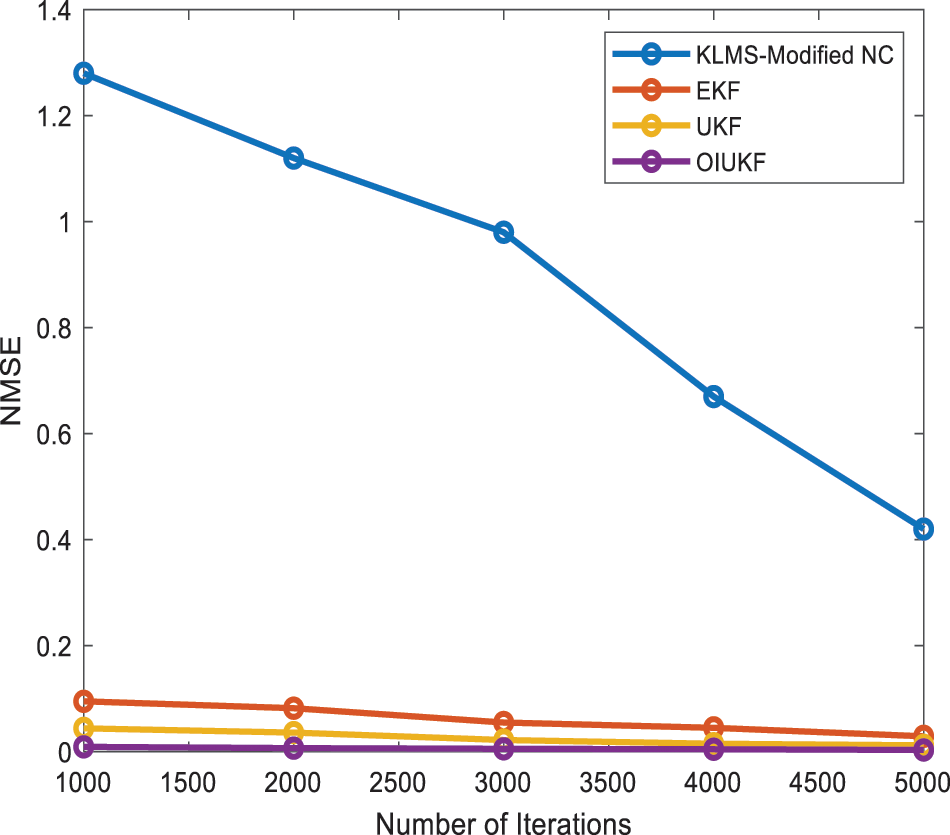
Figure 1: Comparison of NMSE for time delay estimation for scenario 1

In Doppler shift estimation, the proposed OIUKF-based estimation yields a decreased NMSE value of 0.00094, whereas other approaches such as EKFs, UKFs, and KLMS Modified NC give higher NMSE values of 0.36, 0.045, and 0.0092 respectively, after 5000 iterations in scenario 1 as shown in Fig. 2.

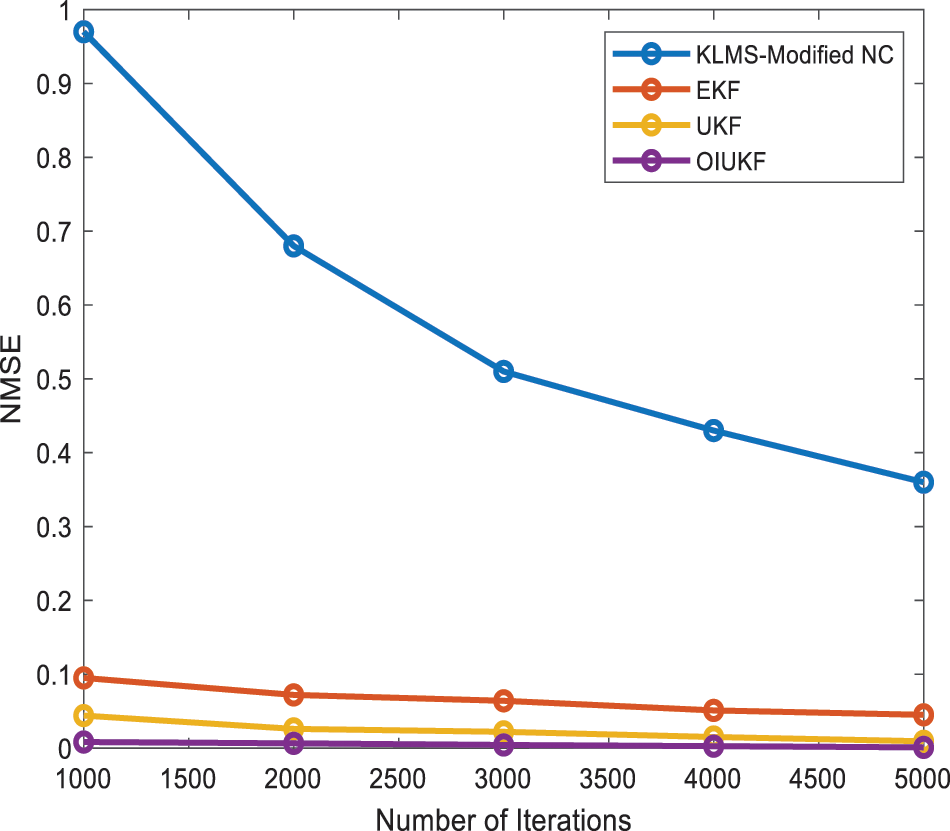
Figure 2: Comparison of NMSE for Doppler shift estimation for scenario 1

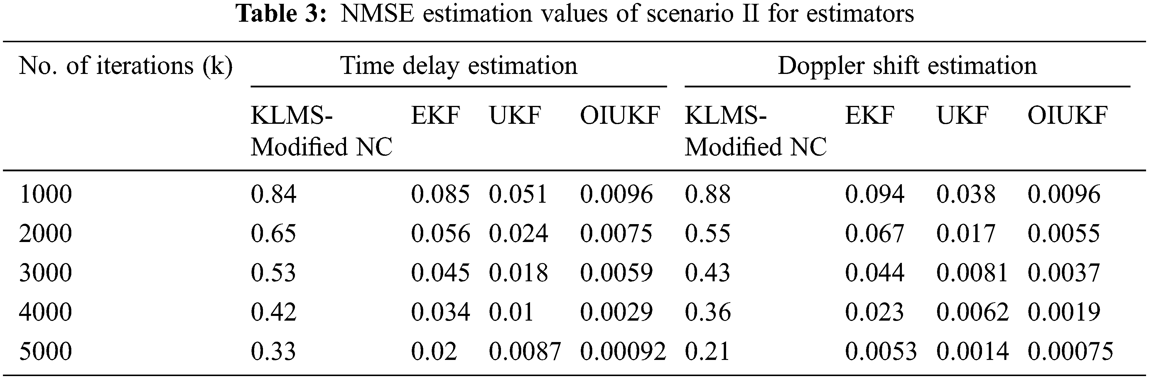
Fig. 3 shows that the proposed OIUKF-based estimation has a lower NMSE of 0.00092, whereas other approaches such as EKFs, UKFs, and KLMS Modified NC have higher NMSEs of 0.33, 0.020, and 0.0087 respectively, after 5000 iterations in scenario 2 in Estimation of TDEs.

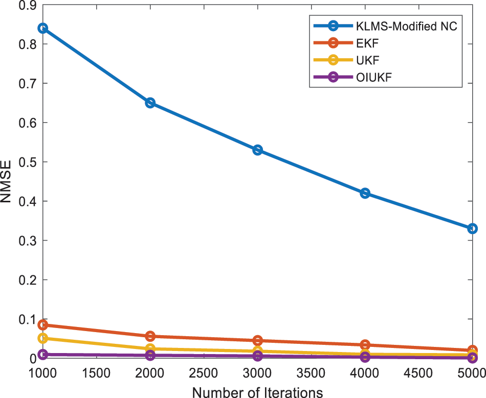
Figure 3: Comparison of NMSE for time delay estimation for scenario 2

According to Fig. 4, the suggested OIUKF-based estimation has a lower NMSE value of 0.00075, whereas other approaches such as EKFs, UKFs, and KLMS Modified NC have higher NMSE values of 0.21, 0.053, and 0.0014, respectively, at 5000 iterations in Doppler Shift estimation [25]. With the suggested estimate methodologies, the decreased NMSE results in better accuracy in TDEs and Doppler shift estimation. Fig. 5 demonstrates the variations acquired from the EKFs, UKFs, KLMS-Modified NC, and suggested OIUKF based estimations. When compared to the KLMS-Modified NC, the variances achieved with the EKFs and UKFs are closer to the attainable OIUKF estimation, as seen in the figures. Furthermore, the statistics show that the UKF’s is somewhat more accurate than the EKFs.

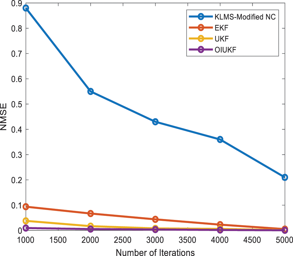
Figure 4: Comparison of NMSE for Doppler shift estimation for scenario 2

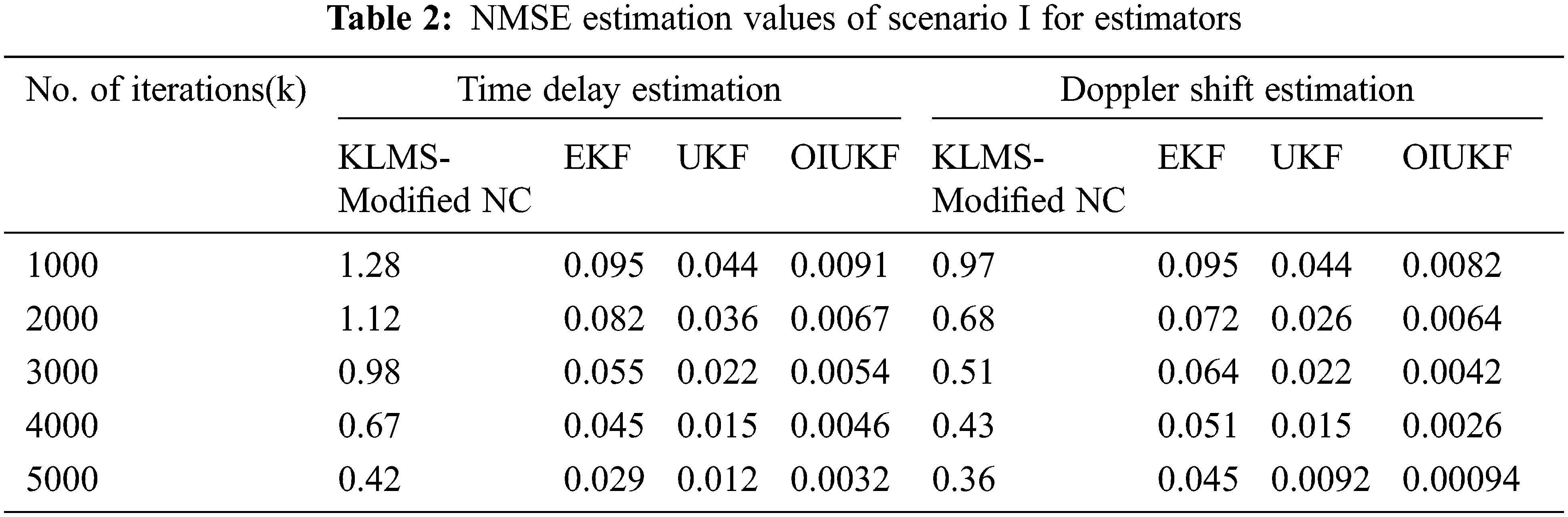
In Fig. 5, established approaches such as KLMS Modified NC and UKFs are compared to EKFs and OIUKF-based estimating methodologies. Furthermore, the variance achieved by the OIUKF-based estimate is much smaller than the variance obtained by the other approaches. At 5000 iterations in scenario 1, the proposed OIUKF-based estimation yields a decreased variance value of 0.00018, whereas other approaches such as EKFs, UKFs, and KLMS Modified NC give increased variance values of 0.92, 0.11, and 0.00089, respectively. The comparison of NMSE for the scenario I and scenario II were discussed in Tabs. 2 and 3 and shows that OIKUF has a minimum mean square error.

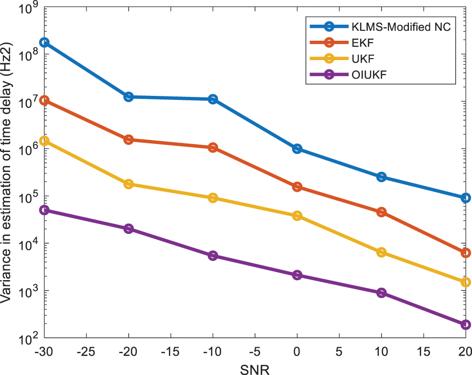
Figure 5: Estimate strategies for scenario 1 variance in time delay estimation based on KLMS-Modified NC, UKFs, EKFs, and OIUKF

4  Conclusion and Future Work

TDEs and Doppler shifts are used in RSs to derive measures like ranges and radial velocities. The proposed OIUKFs and the EKFs are two unique nonlinear estimation approaches that can overcome the estimator’s limitations and with enhanced outcomes for TDEs and Doppler shifts. Nonlinearity is regarded as the genuine nonlinear model for estimation in the proposed OIUKF system. MCEHO is used to optimize a new parameter using a cost function. The OIUKF system uses a numerical approximation to provide a derivative-free implementation. It is more stable than the EKFs since it is implemented without derivatives. EKFs are favourable because of their ease in implementations, but they suffer from inadequate representations of nonlinear functions by first-order linearization, whereas the proposed OIUKFs outperform EKFs while having better stability due to precise treatment of the system’s nonlinearity. As a result, the OIUKFs outperform EKFs in terms of stability and yield estimates that are similar in accuracy. In actuality, however, clutter, which is frequently represented as non-Gaussianity, is common. As a result, future research into the nonlinear form of the Kalman filter capable of dealing with non-Gaussianity to deal with the effects of clutter will be possible. The tracker also requires range, radial velocity, and angle information for accurate tracking.

Funding Statement: The authors received no specific funding for this study.

Conflicts of Interest: The authors declare that they have no conflicts of interest to report regarding the present study.

References

 1.  H. You, X. Jianjuan and G. Xin, Radar data processing with applications. John Wiley & Sons, China, pp. 1–560, 2016. [Google Scholar]

 2.  D. You, P. Liu, W. Shang, Y. Zhang, Y. kang et al., “An improved unscented kalman filter algorithm for radar azimuth mutation,” International Journal of Aerospace Engineering, vol. 1, no. 3, pp. 1–10, 2020. [Google Scholar]

 3.  M. A. Richards, J. A. Scheer and W. A. Holm, “Principles of modern radar,” SciTech Publishing, vol. 1, pp. 1–962, 2010. [Google Scholar]

 4.  N. P. Bhatta and M. Geetha Priya, “Radar and its applications,” International Journal of Circuit Theory and Applications, vol. 10, no. 3, pp. 1–9, 2018. [Google Scholar]

 5.  M. Boutkhil, A. Driouach and A. Khamlichi, “Detecting and localizing moving targets using multi-static radar system,” Procedia Manufacturing, vol. 22, no. 3, pp. 455–462, 2018. [Google Scholar]

 6.  M. Longbrake, “True time delay beam steering for radar,” in IEEE National Aerospace and Electronics Conf. Dayton USA, pp. 246–249, 2012. [Google Scholar]

 7.  U. K. Singh, R. Mitra, V. Bhatia and A. K. Mishra, “Target range estimation in OFDM radar system via kernel least mean square technique,” in Proc. Int. Conf. on Radar Systems, United Kingdom, pp. 1–5, 2017. [Google Scholar]

 8.  G. Y. Kulikov and M. V. Kulikova, “The accurate continuous-discrete extended kalman filter for radar tracking,” IEEE Transactions on Signal Processing, vol. 64, no. 4, pp. 948–958, 2015. [Google Scholar]

 9.  W. Liu, J. C. Principe and S. Haykin, Kernel adaptive filtering: A comprehensive introduction. Vol. 57. John Wiley & Sons, China, 2011. [Google Scholar]

10. I. Santamaria, “Kernel adaptive filtering: A comprehensive introduction,” IEEE Computational Intelligence Magazine, vol. 5, no. 3, pp. 52–55, 2010. [Google Scholar]

11. M. karasalo and X. Hu, “An optimization approach to adaptive Kalman filtering,” Automatika, vol. 47, no. 8, pp. 1785–1793, 2011. [Google Scholar]

12. Z. Ibrahim, N. H. A. Aziz, N. A. A. Aziz, S. Razali and M. S. Mohamad, “Simulated kalman filter: A novel estimation-based meta-heuristic optimization algorithm,” Advanced Science Letters, vol. 22, no. 10, pp. 2941–2946, 2016. [Google Scholar]

13. U. K. Singh, A. K. Singh, V. Bhatia and A. K. Mishra, “EKF and UKF based estimators for radar system,” Frontiers in Signal Processing, vol. 1, pp. 1–11, 2021. [Google Scholar]

14. K. V. Mishra and Y. C. Eldar, “Performance of time delay estimation in a cognitive radar,” in Proc. 2017 IEEE Int. Conf. on Acoustics, Speech and Signal Processing (ICASSP), New orleans, LA, USA, pp. 3141–3145, 2017. [Google Scholar]

15. F. Roemer, M. Ibrahim, N. Franke, N. Hadaschik, A. Eidloth et al., “Measurement matrix design for compressed sensing based time delay estimation,” in Proc. 24th European Signal Processing Conf. (EUSIPCO), Hungary, pp. 458–462, 2016. [Google Scholar]

16. A. Chehri, P. Fortier and P. Tardif, “Time delay estimation for UWB non-coherent receiver in indoor environment, from theory to practice,” EURASIP Journal on Wireless Communications and Networking, vol. 1, no. 1, pp. 1–11, 2018. [Google Scholar]

17. X. Li, W. Cui, H. Xu, B. Ba and Y. Zhang, “A novel method for DOA and time delay joint estimation in multipath OFDM environment,” International Journal of Antennas and Propagation, vol. 2020, no. 3952175, pp. 1–11, 2020. [Google Scholar]

18. X. Li and X. Ma, “Joint doppler shift and time delay estimation by deconvolution of generalized matched filter,” EURASIP Journal on Advances in Signal Processing, vol. 1, no. 1, pp. 1–12, 2021. [Google Scholar]

19. I. Veshneva and G. Chernyshova, “The scenario modeling of regional competitiveness risks based on the Chapman-Kolmogorov equations,” in Journal of Physics: Conf. Series, Russia, IOP Publishing, vol. 1784, pp. 1–13, 2021. [Google Scholar]

20. M. A. Skoglund, G. Hendeby and D. Axehill, “Extended Kalman filter modifications based on an optimization view point,” in Proc. 18th Int. Conf. on Information Fusion (Fusion), Washington, USA, pp. 1856–1861, 2015. [Google Scholar]

21. F. Gustafsson and G. Hendeby, “Some relations between extended and unscented kalman filters,” IEEE Transactions on Signal Processing, vol. 60, no. 2, pp. 545–555, 2011. [Google Scholar]

22. G. G. Wang, S. Deb, X. Z. Gao and L. D. S. Coelho, “A new meta heuristic optimisation algorithm motivated by elephant herding behaviour,” International Journal of Bio-Inspired Computation, vol. 8, no. 6, pp. 394–409, 2016. [Google Scholar]

23. E. Tuba, R. Capor-Hrosik, A. Alihodzic, R. Jovanovic and M. Tuba, “Chaotic elephant herding optimization algorithm,” in IEEE 16th World Symp. on Applied Machine Intelligence and Informatics (SAMI) Kosice, New Jersey, pp. 00213–00216, 2018. [Google Scholar]

24. P. P. Gandhi and S. A. Kassam, “Optimality of the cell averaging CFAR detector,” IEEE Transaction on Information Theory, vol. 40, no. 4, pp. 1226–1228, 1994. [Google Scholar]

25. J. Yan, D. Yuan, X. Xing and Q. Jia, “Kalman filtering parameter estimation techniques based on genetic algorithm,” in IEEE Int. Conf. on Automation and Logistics, China, pp. 1717–1720, 2008. [Google Scholar]

This work is licensed under a Creative Commons Attribution 4.0 International License, which permits unrestricted use, distribution, and reproduction in any medium, provided the original work is properly cited.