Computer Systems Science & Engineering DOI:10.32604/csse.2023.027399
Article

A Highly Accurate Dysphonia Detection System Using Linear Discriminant Analysis

Anas Basalamah1, Mahedi Hasan2, Shovan Bhowmik2 and Shaikh Akib Shahriyar2,*

1Department of Computer Engineering, Umm Al-Qura University, Makkah, Saudi Arabia
2Department of Computer Science and Engineering, Khulna University of Engineering & Technology, Khulna, 9203, Bangladesh
*Corresponding Author: Shaikh Akib Shahriyar. Email: akib.shahriyar@cse.kuet.ac.bd
Received: 17 January 2022; Accepted: 14 March 2022

Abstract: The recognition of pathological voice is considered a difficult task for speech analysis. Moreover, otolaryngologists needed to rely on oral communication with patients to discover traces of voice pathologies like dysphonia that are caused by voice alteration of vocal folds and their accuracy is between 60%–70%. To enhance detection accuracy and reduce processing speed of dysphonia detection, a novel approach is proposed in this paper. We have leveraged Linear Discriminant Analysis (LDA) to train multiple Machine Learning (ML) models for dysphonia detection. Several ML models are utilized like Support Vector Machine (SVM), Logistic Regression, and K-nearest neighbor (K-NN) to predict the voice pathologies based on features like Mel-Frequency Cepstral Coefficients (MFCC), Fundamental Frequency (F0), Shimmer (%), Jitter (%), and Harmonic to Noise Ratio (HNR). The experiments were performed using Saarbrucken Voice Database (SVD) and a privately collected dataset. The K-fold cross-validation approach was incorporated to increase the robustness and stability of the ML models. According to the experimental results, our proposed approach has a 70% increase in processing speed over Principal Component Analysis (PCA) and performs remarkably well with a recognition accuracy of 95.24% on the SVD dataset surpassing the previous best accuracy of 82.37%. In the case of the private dataset, our proposed method achieved an accuracy rate of 93.37%. It can be an effective non-invasive method to detect dysphonia.

Keywords: Dimensionality reduction; dysphonia detection; linear discriminant analysis; logistic regression; speech feature extraction; support vector machine

1  Introduction

The introduction of Machine Learning (ML) in the healthcare system allows different types of diseases to be easily detected. Chronic conditions and emergencies can be diagnosed using modern techniques of ML. Dysphonia is a kind of voice disease that deals with changes in the pitch, vocal cord quality, and loudness of the voice. About 10% of the population suffers from this issue [1], which is caused by bad social habits and other voice abuses. Additionally, some other diseases like puberphonia, cocal fold nodules, or chorditis are also caused by problems with the vocal folds and can be tracked by examining speech feature values. A change in voice quality is the first sign of any kind of voice pathological disorder. Despite revolutionary changes in medical science, there is still some room for improvement in voice disease detection.

Digital processing of voice signals is a non-invasive technique and can be considered as an objective diagnosis to assess voice disorders in a research setting. Many invasive techniques such as stroboscopy and laryngoscopy are employed by physicians for voice impairment diagnostics which can be uncomfortable for patients. Consequently, automatic acoustic analysis can be very useful as an alternative tool for the diagnosis of voice disorders. In our research, non-invasive acoustic analysis can efficiently provide diagnostic quantitative data.

This research aims to evaluate the process and improve the accuracy of the dysphonia detection system. In general, short-time and long-time methods are applied as two categories for feature extraction from the speech signal. Two widely accepted methods, namely Short Time Energy (STE) and Zeros Crossing Rate (ZCR) [2,3], are used as short-time feature extraction methods. In our research however, we used different long-time parameters, such as Fundamental Frequency (F0), Shimmer (%), Jitter (%), Harmonic-to-Noise Ratio (HNR), and MFCC [1,4,5], to evaluate vocal tract health. We present a novel approach to detect the pathological voice sample from a healthy sample by applying Linear Discriminant Analysis (LDA) as a preprocessing step in addition to other ML algorithms for dysphonia detection.

We investigated different algorithms for voice disorder classification and finally developed an efficient structure to improve recognition rate and computational complexity. We have developed a process to improve the accuracy of distinguishing pathological voices from healthy voices by examining different voice features. Our major contributions are:

•   Our research is the first to introduce LDA to dysphonia detection providing a 70% increase in processing speed compared to PCA (see Section 6.7).

•   We analyzed the performance of our proposed algorithm using SVM with both Polynomial and RBF kernel and demonstrate an accuracy of 95.24%, which is a 12.87% increase in performance compared to current state-of-the-art models.

•   We modeled Logistic Regression and K-NN and demonstrate that the proposed model’s accuracy remains in the region of 94.5%, maintaining stability and reliability of the detection accuracy when maximum MFCC features are considered.

•   We utilized a private dataset of voice samples and predicted pathologies of those voices by applying ML models trained by our SVD dataset and had an accuracy of 93.5% using SVM.

This article is organized as follows. Sections 2 and 3 contain the related works and some necessary preliminary discussions on different ML techniques. Section 4 describes our proposed methodology. Section 5 contains a detailed explanation of the experimental studies. Section 6 discusses the results of the experiment. Section 7 shows a brief conclusion of our work.

2  Related Work

With the development of speech and language processing technology, voice analysis is one of the most promising areas of research. Voice features are very effective to identify different vocal diseases. Some common voice features are Fundamental Frequency (F0), Shimmer, Jitter and MFCC (see Section 4). These characteristics have been used for voice pathology diagnosis in many works.

Audio features are used in several studies for voice-related analysis. Speech disability was identified using the MFCC feature matrix as a prerequisite for providing standard telecommunication services by Jhawar et al. [6]. MFCC, Perceptual Linear Prediction (PLP), and Relative Spectral Transform-PLP (RASTA-PLP) are three different cepstral coefficients with five supervised ML models which were applied for discriminating different patients with neurological disorders [7]. Indeed, researchers used signals from 36 pathological patients and 36 healthy patients and successfully determined the relationship of depression with voice features by using MFCC with 78% sensitivity and 86% specificity [8]. Bennane et al. [9] synthesized a pathological voice by employing a DDS-based synthesizer to analyze the effect of Shimmer and Jitter on voice quality. Shimmer and Jitter are also used for Parkinson’s disease detection [10]. Daly et al. [11] further described MFCC, PLP, Shimmer, and Jitter for voice analysis.

Different voice diseases were measured using voice features and by applying various ML algorithms. SVM was exercised for voice disease detection based on MFCC features using only Radial Basis Kernel (RBF) and a small dataset achieved 95% accuracy [12]. The dataset sample was composed of 173 pathological and 53 healthy voices selected from the MEEI database. While the accuracy is high, a small dataset was used and the generalization capability is poor. A mixture of kernels can be useful for better extrapolation [13]. The MEEI database was also used to classify voice pathology using Deep Neural Network (DNN) for 462 voice samples [14]. Nakai et al. [15] measured abnormal prosody in word utterances of children using ML based voice analysis and speech therapy. Parkinson’s disease was also diagnosed using a supervised classification based DNN [16]. A popular voice database, Saarbrucken Voice Database (SVD), was used by Verde et al. [1]. They selected a total of 1370 voice samples of vowel /a/ and considered F0, Shimmer, Jitter, 13-MFCC, First and second derivatives of cepstral coefficient, and HNR parameters. They selected SVM, Logistic Model Tree (LMT), Decision Tree (DT), and Bayesian Classification (BC) as classification techniques. Among them, the best accuracy (85.77%) was achieved by the SVM classifier considering all parameters. They used Principal Components Analysis (PCA) for significant feature selection. Similar research was performed by Dankovičová et al. [17] where 1560 speech features were used to detect dysphonia. Apart from SVM, Logistic Regression is widely used in health-related issues and performs better than other regression models for statistical data [18]. KNN also functions well in health-related classification and signal analysis [19].

Clearly, MFCC is a major voice feature for finding different characteristics of an individual voice. Furthermore, other features are also used for recognizing different voice diseases. The ML approach was exploited for different voice disorder findings of vocal folds, and a deep learning approach was also applied. Dimensionality reduction was done as a preprocessing step and PCA was used. Based on our in-depth look at the current literature, where vocal disease analysis was done and voice features were used as attributes, we can conclude that voice disease was studied on a small scale and the detection accuracy lies below 90% for the larger datasets. Also, most works did not concentrate specifically on dysphonia rather they focused on voice diseases at large. Moreover, the effect of minimum and maximum MFCC features was not studied in the case of dysphonia detection. Considering these findings, we aimed to develop a more accurate (greater than 90%) and robust ML model for finding dysphonia in a non-invasive way. In our work, we used SVM with two different kernels (RBF and Polynomial) not only for MFCC, but also for other features as well, and worked with all features combined. We used both kernels for SVM because it works better for normalized data while applying it to numeric data [20]. In addition to SVM, we also used Logistic Regression and KNN for identifying dysphonia. Our proposed work, based on these three algorithms, outperforms other works related to dysphonia detection. Moreover, we completed our work based on large datasets (approximately 14000 voice signals) with different important voice features like F0, Shimmer, Jitter, HNR, and MFCC. These features have good score level fusion compared to other features [21], and consequently responded well in our experiment.

3  Preliminaries

To classify the pathological voice samples from normal voice samples, SVM, Logistic Regression, and K-NN are used to train the dataset, and therefore the performance of these models is evaluated. These are supervised ML models. For an exhaustive comparison, we have chosen these three different ML algorithms. As previously described in Section 2, SVM kernel functions, RBF and Polynomial, have not been deployed in dysphonia detection. We also explained the motivation behind the preference of selecting Logistic Regression and K-NN algorithms in our study, as both respond better in health-related statistical data prediction. Moreover, these models are widely recognized in classification, especially in binary classification [22], and can be easily deployed in end-to-end devices [23]. We do not need any high-configuration end devices to run these algorithms due to their light computation requirements. In the next subsections, we will briefly discuss the three algorithms.

3.1 Support Vector Machine

This is a binary classifier defined by a separating hyperplane that divides data into different classes. To differentiate the two classes of data points, several feasible hyperplanes that can be chosen. The goal is to achieve a plane with maximum margins, i.e., the largest distance of data points from both classes. Hyperplanes are a decision boundary that help differentiate data points. For detecting voice disease, SVM is a very useful classifier with good accuracy, but it does not work for more than two dimensions. Consequently, we used proper reduction technique to improve classification accuracy by changing different kernel functions. In our experiment we used RBF and Polynomial kernels to train the dataset for our desired output [24]. The kernel functions are given in Eqs. (1) and (2).

RBFk(xi,xj)=exp(||xi−xj||2σ2) (1)

Polinomialk(xi,xj)=(xi.xj+1)p (2)

In Eqs. (1) and (2) xi and xj are two feature vectors. In Eq. (1), σ is a free parameter, and in Eq. (2) p is the degree of the polynomial function. p can be of 0,1, 2, 3,… and so on.

3.2 Logistic Regression

This is a statistical model that uses a logistic function to model the binary dependent variable. This model works well on linear separable groups, which is primarily used where a binary classification problem has a chance of occurring [25], such as the probability of an event occurring. We used the default solver “liblinear” and multiclass “ovr” as the parameters for this model. The following sigmoid function in Eq. (3) is used successfully in our research which takes any real input t (t ð R) and outputs a value between zero and one for the logit.

σ(t)=11+exp−t (3)

The logit function can be described as in Eq. (4) where P is the probability of a positive event.

Logit(P)=log11−P (4)

3.3 K-Nearest Neighbour

One of the simplest but most powerful methods is K-NN. In this model, the class label of a test element is determined according to the class label of the adjacent training data elements [25]. In our work, the similarity between the two elements was measured using ‘Minkowski’ distance. It is a generalization of the Euclidean and Manhattan distance. We empirically chose the value of ‘k’ equals 5, the number of nearest neighbors that must be considered. The Minkowski distance (Dij) of order two, between two input feature vectors (Xi, Xj), is given by Eq. (5) where k = 1, 2, 3, …, n.

Dij=∑k=1n(Xik−Xjk)2 (5)

4  Proposed Dysphonia Detection System

The overall working procedure of our research can be inferred from the following flow chart (see Fig. 1). We collected voice samples containing both healthy and pathological (dysphonia) voices from a well-balanced public database named Saarbrucken Voice Database (SVD) [1,26]. We collected a total of 13992 voice samples of 1166 persons having both voice signals of male and female from SVD. The voice samples were resampled in 48 kHz and the format was in “.wav”. After collecting the voice samples, 13 MFCC feature values were extracted and split into five folds. In each fold, there was an equal number of features inserted. We understand that signals and feature values may consist of exact values as well as some outliers because of the environment and other factors. Thus, we have followed multiple preprocessing steps before applying ML algorithms on those voice features. After splitting into folds, feature scaling was used to normalize the values. Then we reduced the dimensionality of the feature matrix by LDA. After that, we added some other features like Fo, Shimmer (%), Jitter (%), and HNR. These features were selected based on previous studies that leveraged these features specifically to recognize dysphonia [1]. The description of the features are as follows:

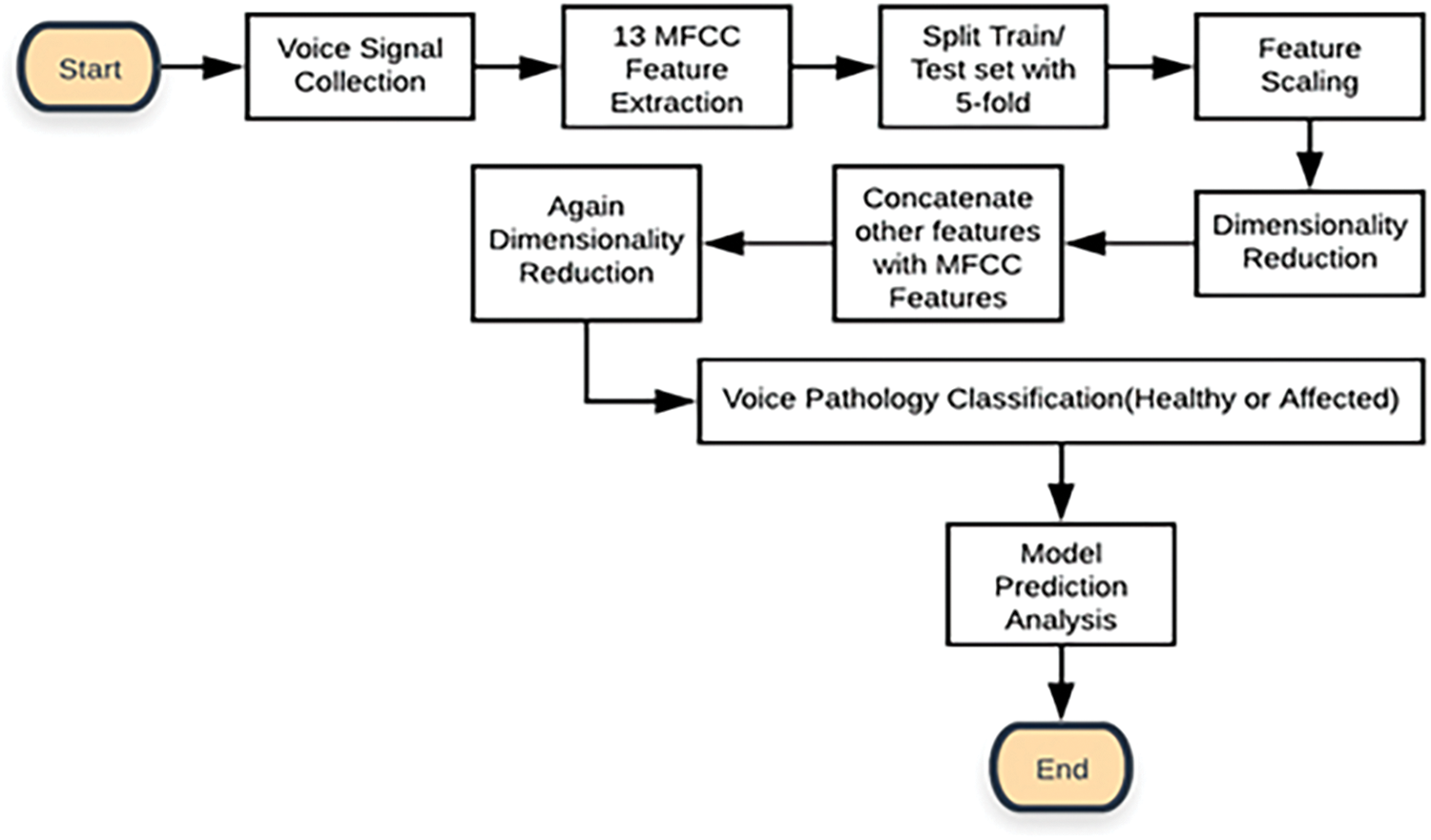
Figure 1: The flowchart of the proposed voice pathology (Dysphonia) detection system

Fundamental Frequency (Fo) is the lowest frequency of a waveform that represents the rate of vibration of the vocal folds forming a special index of laryngeal function.

Jitter (%) mainly describes the unstable oscillation of the vocal folds, measuring cycle-to-cycle changes in fundamental frequency.

Shimmer (%) delineates the unstable oscillation of the vocal folds, measuring cycle-to-cycle changes in fundamental amplitude.

Harmonic to Noise Ratio (HNR) measures the ratio of harmonic sound over noise due to turbulent airflow resulting from an incomplete vocal fold, reasonable for voice pathologies.

Mel-Frequency Cepstral Coefficients (MFCC) are used in the analysis of voice pathologies because they represent the envelopes in the vocal tract. MFCC can help to measure the damage of the vocal folds, the main cause of voice disease. We used 13 MFCC coefficients in our work.

These voice features, F0, Shimmer, and Jitter, can be understood better when by visually analyzing the acoustic audio files of the voice sample [27]. We measured these values using “PRAAT” which is usually used to generate speech reports and for analysis of different speech features [28]. The MFCCs are numeric values of a voice signal and different frames have different numeric values. These values and their dimensionality reduction process is described in Section 5. Fig. 2, generated from “PRAAT”, illustrates the parts of a single voice waveform that are selected to determine voice features like F0, Shimmer, Jitter, and HNR.

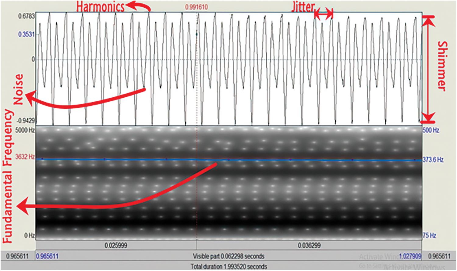
Figure 2: Fundamental frequency, shimmer, jitter, and HNR analysis of an audio file in PRAAT

The fundamental frequency of a voice signal is indicated by a blue signal in the lower portion of Fig. 2 with the value in blue. It denotes the lowest frequency of a particular voice that determines the vibration rate of a voice signal. Similarly, the right upper portion of Fig. 2 indicates which parts are called Shimmer and Jitter of a speech waveform. Cycle to cycle variation in frequency (horizontal difference) signifies Jitter, and a higher percentage of which is a major indicator of voice pathology. The Shimmer is the cycle-to-cycle variation of amplitude (vertical difference), and correlates with noise leakage and the inspiration of a voice. These features are symbolized by red indicators. Finally, HNR is the fraction of the melodic to the coarse part of a speech signal. Since it is the estimation of periodic to non-periodic sound, the highest vibration of a cycle is divided by the previous cycle’s lower vibration to measure the efficiency of the voice. The left upper portion of Fig. 2 exactly shows the harmonic and noisy points of a voice signal which are also specified by a red-colored gauge.

After the concatenation of these features with the MFCC feature values, the overall dimensionality of the features again became high, so dimensionality reduction was reapplied. In this stage, the dataset preprocessing was done successfully. Then we applied the SVM, Logistic Regression, and KNN to build our desired prediction model to detect dysphonia. Since we used the K-fold cross-validation technique, each fold was used both as a training dataset as well as a test dataset in different iterations. After building the models, we checked both using public as well as private data for prediction purposes.

5  Experimental Studies

This section reviews the experimental outcome of our work and how we cascaded the overall task through the setup, database, MFCC feature values, cross-validation, feature scaling, dimensionality reduction, and concatenation.

5.1 Experimental Setup

For our experimental study, we used a desktop computer with a Core-i7-9750H processor (12 M Cache, up to 4.50 GHz) and 8 GB of RAM running Windows 10. The code was developed in Anaconda Package’s IDE “Spyder3” and the scripting language was “Python 3.6”. We used “PRAAT” to extract some acoustic features like F0, Shimmer, Jitter, and HNR.

5.2 Database

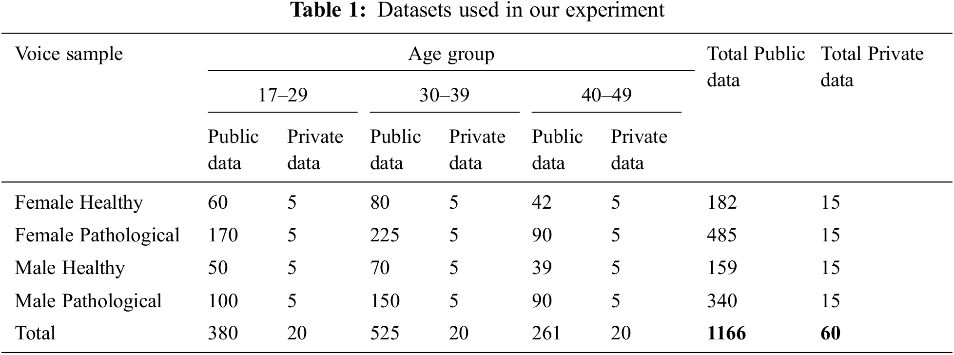
To perform our experimental test on a well-balanced database, we selected 13992 vocalizations from 1166 persons from Saarbrucken Voice Database (SVD) [1,29]. The database contains both healthy and pathological voice samples. This includes four types of voice samples (/a/i/u/a-i-u) of each person. Each voice type has three different levels (low/low-high-low/high). So, there are 12 (3 × 4 = 12) different voice samples for a single person. The voices were sampled at 48 kHz and at a 16-bit resolution. Though the original voices were sampled at 50 kHz, we resampled it into 48 kHz because this is a very common standard sampling rate of voice signals. There are other standard sampling rates such as 44.1, 88.2, or 96 kHz [30]. Among them, 96 kHz sampling rate is considered studio level high-quality voice signal. By selecting 48 kHz, we are inspecting our voice samples to be approximately half of the studio-quality voice signals. The voices were in “.wav” format. We also utilized a private dataset of voice samples provided by ENT Head-Neck Cancer Hospital & Institute [31] to test the stability of our experimental work. We considered the same 12 voice samples (/a/i/u/a-i-u, four types of voice signals with three different levels low/low-high-low/high) from each person. The private dataset contained voice samples from 60 people. These voices were also sampled at 48 kHz and 16-bit resolution. The accumulated voice samples were from three different age groups and two genders. The private voice samples were labeled based on selective measurement, where half of had voice pathologies. After labeling, they were matched with the predicted result. The overall voice signals taken for our research are stated in Tab. 1.

5.3 MFCC Feature Extraction and Matrix Formation

MFCC is a key feature of voice disease analysis. We calculated these feature values by evaluating the discrete cosine transform and the log compression of the voice samples in the frequency domain by using python’s library “librosa” [32]. The MFCC calculation [33] was done as in Eq. (6).

Cm=∑k=1M(log(Sk)∗cos[m(k−0.5)π/M]) (6)

Here, M = total band number, k = i-th band number, Sk = energy of frequency, and m = number of frequency. As the voices were in the “.wav” format, voice samples were variable in length. The MFCC value was calculated for each time frame since MFCC has different length coefficients. These coefficients indicate spectral details of a voice. Based on the sampling rate and bit, the standard coefficient values range from 12–20 [34]. We took 13 MFCC feature values for each audio signal since the 13 MFCC filters can represent the vocal tract envelopes of the human vocal system. In the voice samples, the highest time frame was 208 and the lowest time frame was 7. We created a maximum MFCC feature matrix (13 × 208) taking the highest time frames and a minimum MFCC feature matrix (13 × 7) taking the lowest number of time frames. For the maximum MFCC feature matrix, we used zero paddings for other smaller length values so that there is no N/A in the matrix box. It is found that all the voice samples pronouncing a/i/u start from the beginning of each recording and voice frequency was almost the same for all the recordings. The MFCC values were also near about the same in each case. To analyze whether a small time frame produced good accuracy, we followed the following procedures by taking minimum MFCC feature values as well.

5.4 K-Fold Cross-Validation

After extracting the MFCC feature matrix for all the voice samples, data was split into five folds using the K-fold cross-validation method. This is a statistical method used to estimate the skill of ML models. This approach was used primarily to stabilize the dataset for a proper ML model development [33,35]. In a K-fold cross-validation technique, each fold is used as a training set as well as a testing set in different iterations. Fig. 3 shows the splitting of the dataset into the five folds.

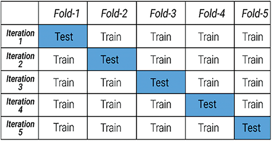
Figure 3: 5-Fold cross-validation

5.5 Feature Scaling

Feature scaling is a method adopted to standardize the range of independent variables or features of data, also known as normalization. The MFCC values were abruptly high for some filters, but to streamline smoothly the computation and reduce the computation load, it is better if the values are smaller. It is also helpful to find the correlation between the MFCC values for the audio signals. Thus, we have used this normalization technique to make the MFCC values smaller.

5.6 Dimensionality Reduction

Dimensionality reduction is the process of reducing the number of random variables under consideration by obtaining a set of principal variables. We reduced our dataset’s dimension by using Linear Discriminant Analysis (LDA) which uses the between-class scatter and within-class scatter for reducing the dimensionality [36]. Whereas PCA has been widely used in image analysis, LDA is rarely used in image classification [37–39]. Nonetheless, LDA works better in acoustic analysis because of the multiplication of within-class and between-class metrics after converting the dataset into 1-D vectors [40]. LDA uses the following two formulas for the between-class scatter SB and within-class scatter SW as stated in Eqs. (7) and (8).

SB=∑classesc2Nc(μc−μ)(μc−μ)T (7)

SW=∑classesc2∑j∈cno. of voices(xj−μc)(xj−μc)T (8)

Here, c = number of classes in the experiment, Nc = size of each class, µc = mean of a particular class, µ = overall mean, xj = feature vector, and T is the degree of the equation. In our study, each MFCC feature matrix (i.e., 13 × 7 and 13 × 208) for a single voice signal was reduced to a 1 × 1 feature matrix.

5.7 Concatenation

After reducing the MFCC feature matrices to 1 × 1, next we merged the other features with the MFCC feature for each voice signal in all the folds, changing the feature matrix to 5 × 1. It was further reduced to the final 1 × 1 feature matrix using the same dimensionality reduction. The overall dimensionality reduction and concatenation procedure are illustrated in Fig. 4.

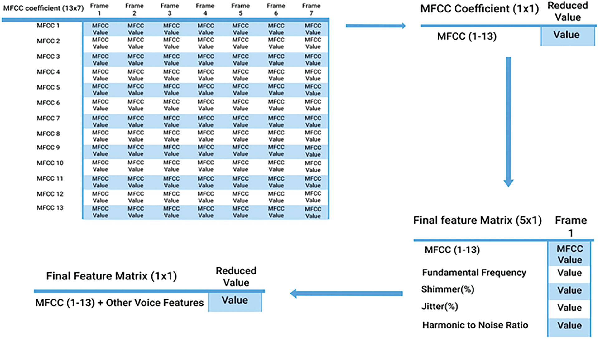
Figure 4: Dimensionality reduction and concatenation workflow

5.8 Fitting into Machine Learning Algorithms

As we collected the voice samples from a valid public database, the class labels were defined in the SVD whether a voice is healthy or disordered. We assigned class labels along with the feature matrix for each voice sample and then fit the training dataset using our earlier mentioned ML algorithms.

6  Experimental Analysis

In this Section, three machine learning algorithms are thoroughly evaluated. We compared these algorithms based on some specific criteria and verified our research work performance by experimenting with two criteria, with and without five-fold cross-validation. We took the features based on two conditions: all features with the maximum (13 × 208) and minimum (13 × 7) MFCC feature matrices. This creates a total of four different results for our research work.

•   True Positive (TP): The voice is pathological, and the algorithm recognizes this successfully.

•   True Negative (TN): The voice is healthy, and the algorithm recognizes this successfully.

•   False Positive (FP): The voice is healthy, but the algorithm recognizes it as pathological.

•   False Negative (FN): The voice is pathological, but the algorithm recognizes it as healthy.

We evaluated the ML models by their accuracy, recall (sensitivity), specificity, precision, F1 measure, and the Area Under the Curve (AUC). These evaluation metrics are well known in binary classification as well as in ML model validation. We have computed all measurements to compare the performance of the different model based on overall SVD and the private dataset. The performance metrics are discussed briefly in the following subsections.

6.1 Accuracy Measurement

Accuracy measurement represents the overall exactness of a model. The Eq. (9) presents the Percent Accuracy computation formula.

Accuracy(%)=(TP+TN)(TP+TN+FP+FN) (9)

6.2 Recall (Sensitivity) Measurement

Recall measurement denotes the classifier’s performance based on false-negative values, also known as sensitivity. In our experiment recall (%) was measured among all the pathological voices, to calculate the number of voices recognized correctly by our algorithms. The formula is provided in Eq. (10) as follows:

Recall(%)=TP(TP+FN) (10)

6.3 Specificity Measurement

Specificity measurement is another measurement technique that was applied in our study. Among all the healthy voices, the percentage of voices detected as healthy can be determined using Eq. (11).

Specificity(%)=TN(TN+FP) (11)

6.4 Precision Measurement

Precision measurement depicts the correct pathological voices based on false positive cases in our experiment. The formula is shown in Eq. (12).

Precision(%)=TP(TP+FP) (12)

6.5 F1 Score Measurement

Additionally, we also calculated the F1 score since our dataset was not completely balanced. F1 score is the harmonic expected value of sensitivity and precision. The formula is given in Eq. (13).

F1Score=2∗Recall∗PrecisionRecall+Precison (13)

6.6 AUC Measurement

Finally, we also calculated the AUC for more acceptance of our model. The AUC portrays the balance between the True Positive Rate (TPR) and the False Positive Rate (FPR). It represents a region under these two values in a 2-D graph. We calculated it in our experiment using sklearn.metrics.auc with a threshold value of one [41]. The overall performance of our experiment is presented in Tab. 2.

6.7 Result Analysis

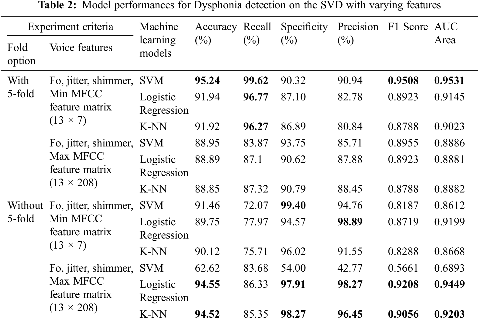
Based on the working process described in the previous section we evaluated our work based on distinct criteria and achieved a very promising result. From the results of Tab. 2, it is apparent that our proposed model fits well to the datasets. We have obtained efficient performance while applying SVM to the minimum MFCC feature matrix along with other features. The recall, specificity, and precision results look encouraging as well, which indicates that our model can successfully discern voice pathologies compared to false-negative and false-positive results. Outside of these measurements, an F1 score of 0.9508 specifies that this model is also performing well in this non-linear unbalanced dataset.

We have also reached a high AUC area close to one, similar to the F1 score. This result indicates our work is sophisticated and that the model is well suited for the desired output. Except for SVM, other algorithms also worked well for both criteria of with and without cross-validation with both maximum and minimum MFCC feature value matrices. Each model achieved high accuracy, recall, specificity, precision, F1 score, and AUC. Our evaluation metrics had an maximum average of 85% to 90% efficacy in predicting dysphonia. F1 and AUC values were, on average, greater than 90%. In all but one case, the work ran smoothly without any complexity.

Previously, in some research, only a single vowel /a/ was used for prediction [1,17], which may result in less accurate predictions. In our work, we selected voice samples of three vowels (/a/i/u/) from separate .wav audio files since some people may pronounce ‘/a’ without difficulty but suffer more when pronouncing ‘/i’ or ‘/e’ or ‘/u’. Therefore, if we take more syllables, it will represent a more real-world scenario. Using three vowels for our experiment helped to generalize the overall working capacity of our model. Therefore, if any person has a problem with a single vowel, utterances of other vowels can help him/her to accurately determine the voice pathology.

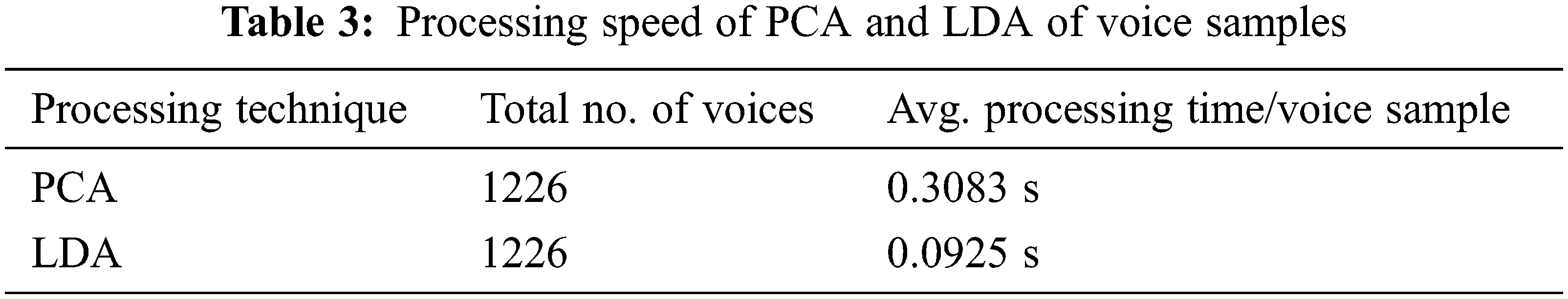
Additionally, PCA was used for dimensionality reduction of extracted voice features using LDA [1,17]. LDA works well when the dataset is large, and it holds the class value more precisely with larger datasets [42]. The usage of LDA for dimensionality reduction helped us to reserve the main component values without any perceptible error. Both SVD and the private dataset had a moderately large number of voice samples in each class. Since PCA performs well when the number of samples per class is low, LDA is particularly advantageous. We have generated a scatter plot for the most significant two features of both PCA and LDA on SVD. Fig. 5 portrays the scatter plot and shows that LDA could easily separate the two classes. Whereas PCA fails to separate the two classes and the features overlap significantly. The average processing times of PCA and LDA on the total 14712 voice samples are shown in Tab. 3. As Tab. 3 suggests, LDA has a gain of 70% in processing speed when compared with PCA. In the real-world application, where diagnosis time of symptoms is crucial, the reduction in the processing time of voice samples gained by the LDA gives our proposed dysphonia detection system beneficial.

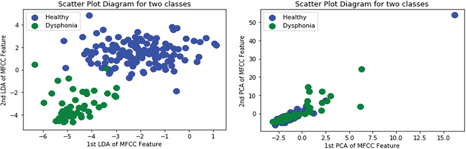
Figure 5: Scatter Plot Diagram for PCA and LDA Features

Moreover, we used the logistic regression model for this research work. It helped us analyze the voice-related pathology concerning other models with good accuracy. While other previous experiments did not use logistic regression, we found that it gave more than 90% accuracy with high recall, specificity, precision, F1 score, and AUC. Again, K-fold cross-validation is also new in this work. Previously only training and test data split operation was done. So, it gives our model more validity and justifies its performance.

Our model depicted great performance in detecting positive diseased results as well as healthy voice samples. However, considering MFCC, F0, Shimmer, Jitter, and HNR, our best result is 95.24%, with the previous best being 82.37% [1] on the SVD database. Among the 12 models, only one model performed poorly, the SVM model without cross-validation with feature matrix size 13 × 208. We assume the support vector was not properly fitted to that particular case’s feature space. The graphical representations of the accuracy of our models are drawn in Figs. 6 and 7.

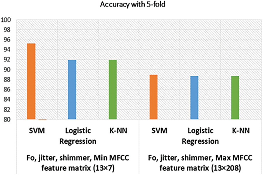
Figure 6: Accuracy of models with cross-validation

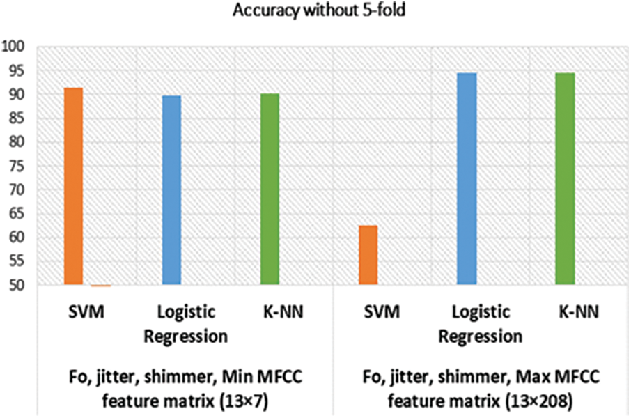
Figure 7: Accuracy of models without cross-validation

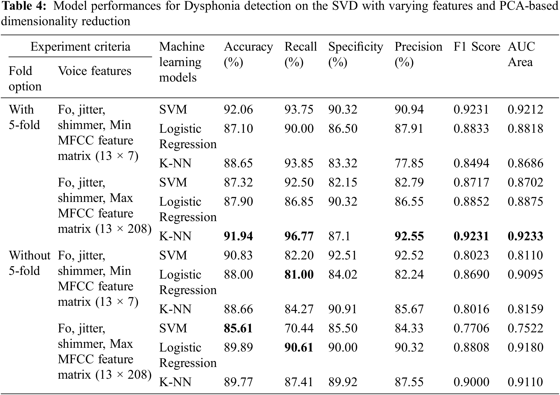
Compared to LDA, we have also tested the performance of the same 12 models leveraging the PCA-based dimensionality reduction technique. The performance of these models is shown in Tab. 4. Overall, the PCA-based models have lower performance metrics than their LDA counterparts except for two cases. Firstly, K-NN performed better (91.94%) when cross-validation and maximum MFCC features were considered. Secondly, SVM performed better (85.61%) when only maximum MFCC features were considered without cross-validation. We suspect this performance gain was due to the creation of higher dimensional hyperplanes by SVM on the maximum MFCC features. Nevertheless, the PCA-based models are still undermined by the LDA-based models.

In this study, we took many voice samples and fitted different features and class labels using prominent and simple to use ML algorithms to build a dysphonia detection model. We have availed different variations of low-high-low frequency level voices which were taken for different vowels from SVD. Nonetheless, a portion of voice was taken from a private dataset consisting of voice samples from people with and without dysphonia and received very promising results.

As previously mentioned, our selected voice features have good score level fusion [21], meaning these selected features are more useful features for voice pathology detection. The utilization of these features helped improve accuracy and performance based on the three ML algorithms. One can easily utilize our proposed ML models either by desktop application or by deploying them at edge devices such as a smartphone or tablet. The model can be incorporated into an application and end-users can easily use the application for early detection of dysphonia without even going to the hospital. Overall, our proposed model can help users make an informed decision to improve their vocal health using the correct treatment plan.

In the case of privately collected data, the performance of SVM trained on our proposed method is compared with our earlier performance on the SVD dataset in Figs. 8 and 9. The accuracy of SVM on the private dataset dropped 1.87%. The recall, specificity, precision, F1 score, and AUC values also follow a similar trend. The private dataset closely resembles voice recordings collected in real-world scenarios in contrast with SVD voice samples, which were collected in a lab setup. Thus, 93.34% accuracy on the private dataset is quite a notable result which signifies our model’s performance stability in real-world voice diagnostic scenarios.

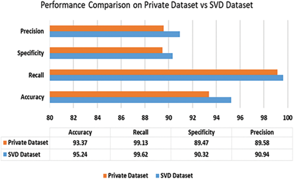
Figure 8: Performance of SVM (ours) on private dataset vs. SVD dataset

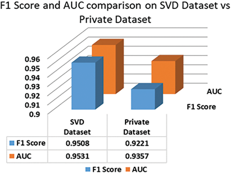
Figure 9: F1 Score and AUC area comparison of SVM on private dataset vs SVD dataset

7  Conclusion

Dysphonia is a voice disease that deals with changes in the pitch, vocal cord quality, and loudness of the voice. Currently, the detection speed and accuracy of the available dysphonia detection systems are unsatisfactory. This motivated development of a process to improve the accuracy of distinguishing pathological voices (voices that have dysphonia) from healthy voices by examining different voice features. We tested our proposed method to predict and analyze voice pathologies from both a standard dataset (SVD) and a private dataset. Our proposed method performed well in both datasets with 95.24% and 93.37% accuracy, respectively. We used LDA for dimensionality reduction and trained SVM, logistic regression, and K-NN classifier to classify and predict voice pathologies. Among them, the SVM model worked best without using DL and only using a lightweight ML algorithm, and our proposed LDA-based training method’s result overcomes the previous low accuracy in this voice disease identifying works. Our prime objective was to develop an ML model that would achieve better accuracy with faster processing speed. Our study has some limitations. We did not utilize other ML classification algorithms like Decision Tree, Naïve Bayes, or Logistic Model Tree. Also, we did not apply DL algorithms. The performance of our proposed methods on the private dataset can be improved if we had collected more voice samples. Additionally, dysphonia is not the only detrimental disease, but there are other diseases of the voice. Thus, further study is needed in this research area. Our future work will focus on applying other prominent ML algorithms along with different DL algorithms, such as Artificial Neural Network (ANN) and Long Short-Term Memory (LSTM) Network. We also plan to use a hybrid DL model to accurately classify voice pathology for not only binary classification, but also for other different classes of voice pathology. Apart from these shortcomings, our proposed model worked comparatively well for detecting dysphonia using LDA with more effective results. We developed a more relevant and efficient process that can detect voice pathology faster and more accurately than previous works. Furthermore, our research work can be deployed to edge devices or as applications. Patients can use this model to diagnose voice pathology in a non-invasive way.

Acknowledgement: We would like to cordially thank the executive committee members of the ENT and Head-Neck Cancer Hospital & Institute for providing us access to their private dataset and helping us to test our developed models.

Funding Statement: The authors received no specific funding for this study.

Conflicts of Interest: The authors declare that they have no conflicts of interest to report regarding the present study.

This work is licensed under a Creative Commons Attribution 4.0 International License, which permits unrestricted use, distribution, and reproduction in any medium, provided the original work is properly cited.