Computer Systems Science & Engineering DOI:10.32604/csse.2023.027612
Article

Human and Machine Vision Based Indian Race Classification Using Modified-Convolutional Neural Network

Vani A. Hiremani* and Kishore Kumar Senapati

Department of Computer Science & Engineering, Birla Institute of Technology, Mesra, Ranchi, 835215, Jharkhand, India
*Corresponding Author: Vani A. Hiremani. Email: vani.hiremani@gmail.com
Received: 21 January 2022; Accepted: 06 April 2022

Abstract: The inter-class face classification problem is more reasonable than the intra-class classification problem. To address this issue, we have carried out empirical research on classifying Indian people to their geographical regions. This work aimed to construct a computational classification model for classifying Indian regional face images acquired from south and east regions of India, referring to human vision. We have created an Automated Human Intelligence System (AHIS) to evaluate human visual capabilities. Analysis of AHIS response showed that face shape is a discriminative feature among the other facial features. We have developed a modified convolutional neural network to characterize the human vision response to improve face classification accuracy. The proposed model achieved mean F1 and Matthew Correlation Coefficient (MCC) of 0.92 and 0.84, respectively, on the validation set, outperforming the traditional Convolutional Neural Network (CNN). The CNN-Contoured Face (CNN-FC) model is developed to train contoured face images to investigate the influence of face shape. Finally, to cross-validate the accuracy of these models, the traditional CNN model is trained on the same dataset. With an accuracy of 92.98%, the Modified-CNN (M-CNN) model has demonstrated that the proposed method could facilitate the tangible impact in intra-classification problems. A novel Indian regional face dataset is created for supporting this supervised classification work, and it will be available to the research community.

Keywords: Data collection and preparation; human vision analysis; machine vision; canny edge approximation method; color local binary patterns; convolutional neural network

1  Introduction

Inter-class classification problems like classifying Indian face vs. Chinese face [1] are pretty feasible than intra-class classification problems like Indian face vs. Indian face [2]. This problem is more apprehensive in a highly populated and diversified country like India, where every region epitomizes different cultures and traditions. Over the years, humans have showcased clever proficiency in judging age, gender, behavior, state of mind, and race by face, even under many obstacles [3–6]. The human brain processes visual statistics in semantic space by extracting the semantically imperative features such as contour information, line segments, edges which are hard to detect by computers. In contrast, machines process them in data space obtained by the strongly detectable but less informative features like texture patterns and chromatic information [7]. Knowing how a human extracts the features can empower diversified artificial intelligence applications employing human-like performance. To explore this, we have proposed an AHIS involving untrained identifiers selected at random in a fine-grained race classification problem to evaluate the potential of human vision. The interrogation of identifiers on given regional face images showed the influence of local conventional facial features like face shape, skin tone, eyebrows, the shape of eyes, orientation of mouth, shape of the nose, and non-conventional features like the style of dressing, vermillion color, and style, draping sari as per regional tradition, physic, mustache, accessories like jewelry and regional amulet thread. This rich feature set will be a reference input set to train neural models for solving computer vision problems. The insight of non-conventional features definitely would suffice the absence of conventional features. Augmentation of these symmetric features can bring tangible gain in classification. The experimental results of human visual analysis have shown an accuracy of 88% when both identifiers and persons in the image are from different regions [8]. 96% accuracy is achieved when both are from the same region [9]. This familiarity of faces [10] reinforced improved performance in classification. The proficiency of humans in underlying classification problems is systematically measured, and the derived discriminative features are characterized through computer vision algorithms using a novel face database. This work emphasizes the strength of CNNs since they have achieved commendable success in image classification on large-scale datasets for a long time [11]. CNN’s are made up of neurons that have learnable weights and biases. They compare the image patch by patch, typically 3 × 3 or 5 × 5 matrices. Each neuron receives some inputs performs a convolution operation between a 3 × 3 patch of image and 3 × 3 filters. The strength of CNN is that they learn local patterns of images rather than global patterns like densely connected layers do. ConvNets learn spatial hierarchies of patterns progressively from abstract to complex features layer by layer. Since patterns are translation invariant, the neuron in a layer is only connected to a small portion of the layer ahead of it. This mechanism reduces the number of computing parameters. Upfront the success of the AlexNet has tremendous influence in the classification process employing sinking filter size [12] or escalating the network deepness [13]. CNN model training is a global optimization problem. We proposed different variations to improve the traditional CNN model to achieve the best fitting parameters by three aspects: Inception module, spectral pooling, and leaky ReLu activation function. The comparative analysis of proposed M-CNN against conventional computational models has shown approximately 92.98% accuracy. Alongside to explore the perceptual annotation of individual feature influence in the overall face, face contour information is obtained from the canny edge detection approximation method and characterized through the CNN model. To this end, a large set of regional face database is created to address the scarcity of region-wise labeled Indian face databases. This database is made public for further research work in addition to relatively available few datasets [14,15] of Indian faces with no regional information.

The main contribution of the paper is as follows:

•   We have developed an automated human intelligent system incorporating 120 identifiers to estimate human vision proficiency. Both conventional and non-conventional features are recorded, which will be prospected as a reference input set to train neural models for solving computer vision problems.

•   We propose variations to the conventional CNN model based on the empirical experiments by including the Inception module, spectral pooling, and leaky ReLu activation function. The statistical hypothesis testing and comparative analysis have shown that the proposed M-CNN model outperformed other conventional models in accuracy and execution time.

•   We present the substantial perceptual annotation of individual features influence in the overall face by obtaining face contour information through canny edge detection approximation method and characterized through CNN model.

•   We have developed a novel Indian regional face database consisting of 2895 faces acquired from north, east, west, and south via online and offline mode. It is labeled database emphasizes a supervised classification problem. It will be available for the research community.

The rest of the paper is organized in the following sections: Section 2 details the proficiency of both humans and machines in race classification in the past. A broad elaboration of materials and methods used in this research work is in Section 3. Section 4 explains the evaluation metrics and analysis of results attained from both humans and machines. Section 5 concludes our work to an extent and details the scope of future work.

2  Related Works

Geographical regional faces do have a stereotyped structure with many discriminative features. Humans and machines systematically process them, applying learning experience and computational logic. In 2009, the racial classification of Caucasian, Black, and Asian abrasive races and gender [16,17] was performed precisely using computer vision. In [18], silhouetted face profiles are given to human identifiers exhibiting a lot of ethnicity information, and based on shape and color, gender is decided. Classification problem becomes handy with subtle feature variations, i.e., finer grained race such as Chinese/Japanese/Korean [19], Chinese sub-ethnicities [20], and Myanmar [21]. In this section, the different inter and intra-class classification problems are discussed, and how human vision has always been influential on machine intelligence in solving computer vision problems is seen. Classification of coarse races such as Caucasian/Black is performed at both human and machine sides with 70%–80% accuracy. Humans can reliably judge the region of a person based on skin complexion, the way the person behaves, facial makeup, accessories, or fashion sense like dressing style and hairstyle. Like humans visualize the input image, divide it into distinct regions, extract the area of interest out of the whole image and validate positioned face, the machine also pursues the image in the same way. It visualizes low-resolution images using low pass filters, segments them into the distinct region using a segmentation algorithm, and extracts a region of interest (ROI) from the image using an object detecting algorithm. Finally, the given face image is verified [22]. In [23], Caroline E. Harriott et al. have proven that more or less human and machine practices the same tactics to do a job by pairing human-machine and human-human participants to find a suspicious thing in an artificial setup. In [24], Kun Yu et al. have developed a human-computer interaction system to help physically challenged people. The way human learns face gestures based on facial features a set of interactive gestures are designed using Face++ to train a machine to achieve interaction with the computer. In [25], Zhihao Shen et al. have trained the machine to boost human-robot communication by inferring the human traits such as eyesight, body gesture, energy, pitch, and Mel-Frequency Cepstral Coefficient (MFCC) through human-robot interaction. In current intelligent manufacturing systems, the human-machine interaction process has become the most crucial aspect, extending to autonomous systems where human trust dynamics can be utilized to improve the human– machine interaction process. Computational models like Local binary patterns, Gabor filters bank, and wavelets are feature extraction schemes performed with excellence like humans [26]. Features play a very vital role in computer vision problems. Selecting the most informative features yields radical improvements in the classification rates. Artificial intelligence is explored to mimic the tasks of human brains in solving science and engineering problems [27]. CNN is being used on a large scale to train machines with massive samples for feature learning. CNN is at the top and outperformed other computational models in classifying Chinese, Korean and Japanese faces.

The survey has described the influence of human intelligence in solving computer vision problems like face recognition, gender classification, object detection, sentiment analysis, and many more. However, these problems fall under inter-class problems where umpteen numbers of features exist to classify the input. The state-of-the-art unveils scarcity of intra-class classification where limited discriminant features are available. This work has encouraged us to address this challenge by proposing a model incorporating humans and machines in racial classification.

3  Materials and Methods

The human and machine-centric face classification architecture is depicted in Fig. 1. It consists of 3 principal parts: (1) Database creation, (2) Automated human intelligence system, and (3) Machine intelligence system (MIS).

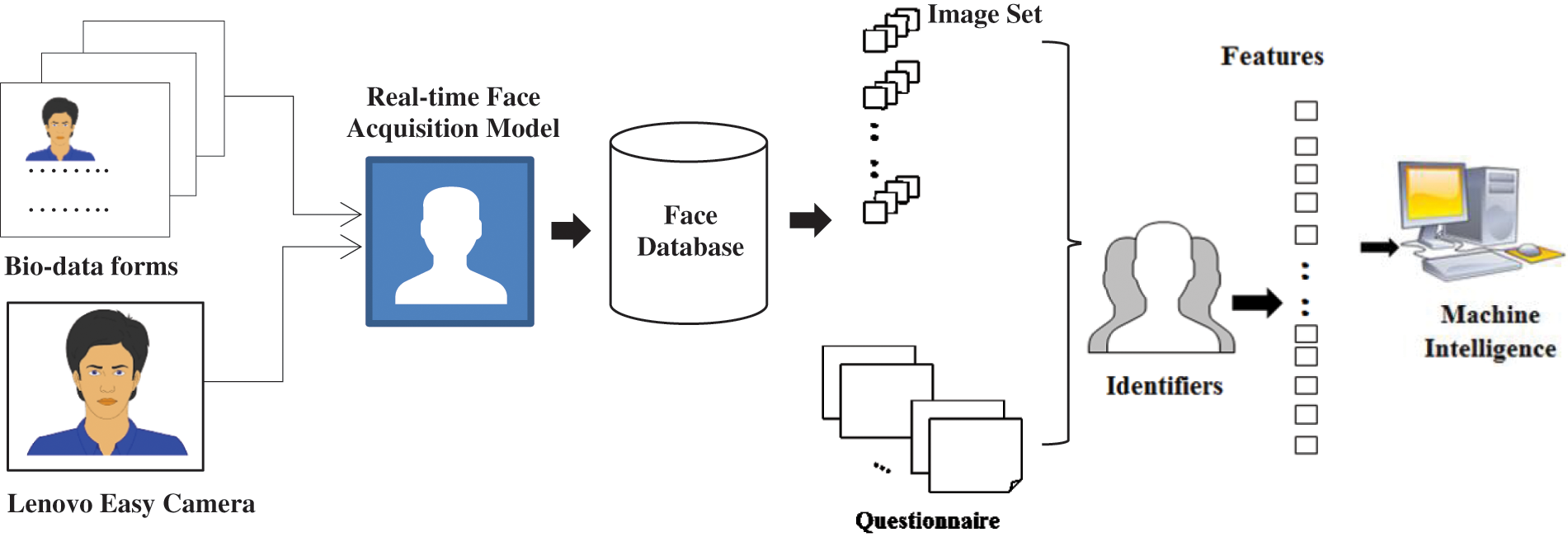
Figure 1: The proposed model describes three parts: 1. Face images are acquired through static and dynamic mode to create Indian face database. Pre-processing is handled at this stage (only cropping is performed under pre-processing). 2. Each identifier is interrogated against a set of 10 face images along with questionnaire form. 3. Computational models are used to characterise the feature and the approach used by human to classify human face to particular region

3.1 Data Pre-processing and Annotation

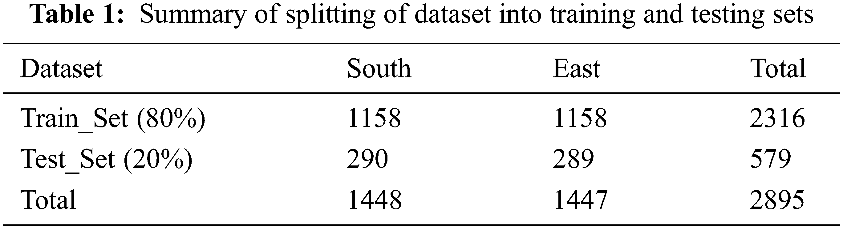
A novel Indian color face database is created to mitigate the scarcity of regional and labeled face images for the underlying supervised classification process. We have sought permission from many universities running in the east and south regions. After receiving the consent, the face images of faculties, staff, students, and their family members are collected through two modes: online (real-time user interface model) and offline (Bio-Data forms with consent disclaimer). The face images are acquired from various states belonging to the east and south regions. An automated face acquisition model is developed to capture real-time face images under candidates’ consent. To capture images, we have used a Lenovo Easy Camera of 2 mp with an aspect ratio of 1.33 and a resolution of size 640 × 480. The candidate is positioned in front of the Lenovo easy camera, the undecorated room wall being in the background. The region of interest (ROI) is detected through the Viola jones algorithm and captured to the size 250 × 350. In offline mode, the scanned Bio-data forms containing candidate photos with minimal information are collected from various universities. These segmented images are then browsed through the automated face acquisition model where the unnecessary background and labeled information are removed, and only ROI is captured to the size of 250 × 350. Around 2010, images acquired from these modes are stored with the primary key as Region_Number (e.g., EAST_01). Images are pre-processed beforehand instead of direct feeding to CNN. A one-hot encoded vector is generated from the categorical name of images. The dependent variables, i.e., labels, are encoded for machine understanding as the dataset consists of categorical names (i.e., SOUTH_01 and EAST_01). The dataset consists of varying size images, so the different resolution images are reduced to the size 50 * 50 pixels and converted into grayscale [28] images to curtail processing speed. 80% of images are considered for training, and the remaining 20% for testing. The following Tab. 1 shows the summary of the dataset split. The Train_Set and Test_Set images are reshaped to size (−1, 50, 50, 1) to fit in TensorFlow.

3.2 AHIS Model: Classification Task

This section describes an empirical examination carried on humans to analyze and understand which features they considered to classify given faces to their regions. Let S be a human intelligence system consisting of input image Ii (picked from I2895 (face database)), questionnaire Q (set of 9 questions, i.e., Q = {q1……… q9}), feature vector Fe (Fe = {f1, f2…….… fL}) [8] extracted by human identifiers, answer A (the subset of features Fe in terms of answers, A ⊆ Fe), and C the result of binary classification (w1 and w2). The representation of AHIS(S) is described as S = {Ii | Ii € I2895, Q, Fe, A, C}. For the given classification task of C and unknown patterns represented by feature vector Fe, we computed conditional probability P as P (wi | Fe), where i represents two classes. After all instant represents the probability that the unknown pattern belongs to the respective class wi, given that the feature vector incorporates the features from Fe. Let’s say w1 and w2 are the two classes consisting of expected patterns. The priori probability P (w1) and P (w2) are estimated from the available training feature vectors. Suppose N is the total available training pattern and instance N1, N2 ⊆ N. If (N1, N2) belong to (w1, w2) respectively then, P (w1) ≈ N1/N & P (w2) ≈ N2/N. The classification now can be stated as,

If P (w1 | Fe) > P (w2 | Fe), Fe is classified to w1

If P (w1 | Fe) < P (w2 | Fe), Fe is classified to w2

Let R1 be the region of the feature space which we decide in favor of w1 and R2 be the corresponding region for w2. Then error is made if F € R1, although it belongs to w2, or if F € R2, although it belongs to w1. That is,

Pe = P (F € R2, w1) + P (F € R1, w2)

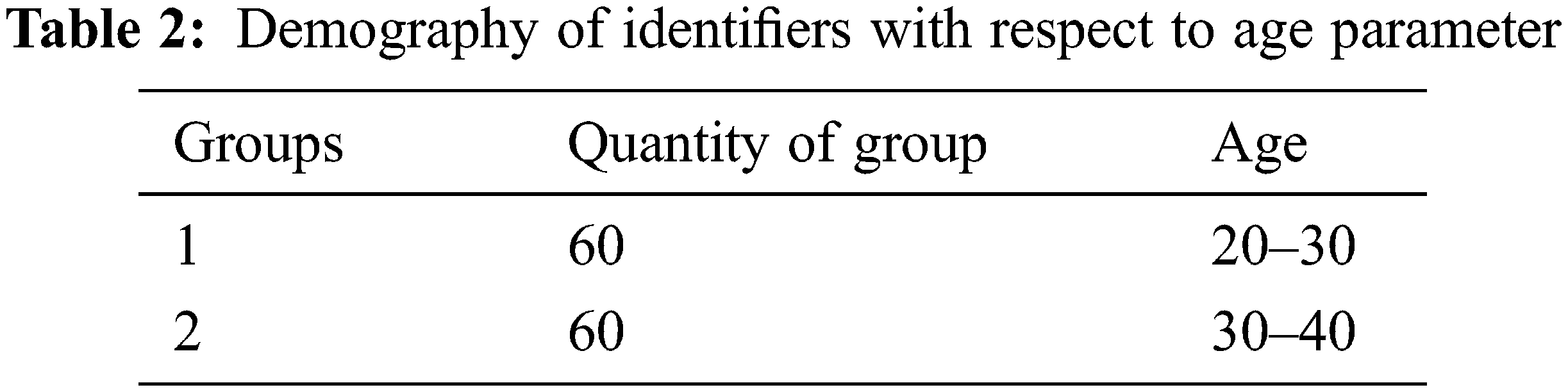
Pe is the joint probability of the P (F € R2, w1) and P (F € R1, w2) events. Fe’s outstanding features are utilized for training the model for further classification. In AHIS, a sample of 120 (shown in Tab. 2) untrained identifiers is selected randomly from various regions of India. Each candidate knows the motto of their contribution beforehand the interrogation to upholding ethical and participatory research.

3.2.1 Human Interrogation

During this phase, the randomly considered identifiers are questioned to their intellect. As shown in Fig. 1, around 2316 images among 2895 are arranged in 122 sets. Each identifier is given a set consisting of ± 19 images. Each identifier is interrogated with a set of fundamental questions [8] and images. The questions are framed to record how the identifier perceives an image, the gender, the discriminating features, and any additional factors those favored identifiers to guess the region.

3.2.2 Feature Analysis

The digitally signed filled forms are meticulously evaluated in this phase. Every identifier has found images adequate for identification, despite challenging images. Despite the absence of any regional accessories, identifiers still decided the correct region looking upon facial features like light complexion, space between eyebrows with small eyes, lightly shaded eyebrows, and marginally sunken cheekbones in case of extreme east regions face. Each identifier’s 10 questionnaire forms are evaluated thoroughly and recorded in an excel sheet incorporating identifiers region, information of images given to them, identified facial features, area of the image identified, its validation, and overall accuracy. The records collectively revealed many facts to human proficiency in identifying the Indian regional people. Two significant observations are made: 1. Identifiers have observed not only conventional face features but also considered non-conventional features. 2. The factor of belonging to the same region played a significant role [9]. 3. The identifiers who mentioned face shape as a promising feature to classify were unable to express what they meant by face shape. Few answers suggested that it is not the shape but the face’s aura or depiction of look that classifies them to a particular region.

To address this limitation at human side the machine vision is explored to characterise this face shape.

3.3 MIS Model: Classification Task

This section describes the computational models like Color local binary pattern (CLBP) and CNN. We improved the feature extraction scheme, Local Binary Patterns (LBP), by adding color factor to it. CLBP is used to comprehend the features observed by identifiers. According to [27], neural networks are best suited for mimicking human intelligence. Therefore we have built two CNN models, CNN-FC and M-CNN. The CNN-FC model is trained with 2316 contoured images obtained from the canny edge approximation method. The M-CNN model also trained with 2316 standard face images to characterize the overall features drawn at the human side.

3.3.1 Color Local Texture Features Extraction

Feature extraction is a crucial step in every computer vision problem. Due to discriminative power and computational simplicity, the LBP texture operator is considered a more stature feature for face recognition. The critical application of the LBP operator is its robustness to monotonic grayscale changes caused (i.e., illumination variations). This LBP operator is applied to the color face image to transform it into a CLBP image. The CLBP image is blocked into 256 cells (16 × 16), i.e., each cell consists of 8 × 8 pixels resolutions. Initially, the space structure of the face is reserved. Then for each square, the LBP histogram is calculated to statistically reflect the edge sharpness, flatness of region, existence of unique points, and variety of local region attributes. Then to each block of the color image LBP function is applied [28]. The LBP feature vector is the concatenated serial of all 16 × 16 intensity values computed from the histogram generated using Y, R, G, and B color components of individual instances of the images. Therefore, the LBP feature is a statistical texture description of the image consisting of a series of histograms of blocked sub-images. The feature dimensions are determined by blocking number and the sampling density. Hence, the size of the template for 100 users is 10000 × 256. During the construction of the LBP feature vector, the bilinear interpolation method is adopted on the LBP grid to estimate the values of neighbors that do not fall precisely on pixels. Since the correlation between pixels decreases with distance, more texture information is obtained from local neighborhoods. We have considered a 300 face image dataset consisting of 5 different images of 60 people from the east and south region. 4 images out of five are trained, and one is tested. The global features are also preserved to retain ample scale information of the image to avoid deformation of images of a person. The CLBP features of trained images are matched against CLBP features of a testing image using Manhattan distance-based algorithm.

3.3.2 CNN-FC

CNN’s are the type of feed-forward Artificial Neural Networks. The output of such a neural network for any input pattern zp is calculated with a single forward pass-through network in Eq. (1). For each output Ok, we have (assuming a few hidden layers in between the input layer and output layer),

Ok,p=fOk(netOk,p)            =fOk(∑j=1J+1.wkjfyj(netyj,p))            =fOk(∑j=1J+1.wkjfyj(∑i=1I+1.vjizi,p)) (1)

where fOk and fyj are the active functions for output Ok and hidden layer yj, wkj is the weight between output Ok and vji. zi, p is the value of input zi, the (I+1)th input unit and the (J+1)th hidden unit are bias units representing the threshold values of neurons in further layer to adjust the weight.

The essential components of CNN-FC are (1) Convolutional Layers, (2) ReLU Layers, (3) Pooling Layers, (4) Fully connected layers, and (5) Dropout layer. Fig. 2 represents the architecture of CNN-FC.

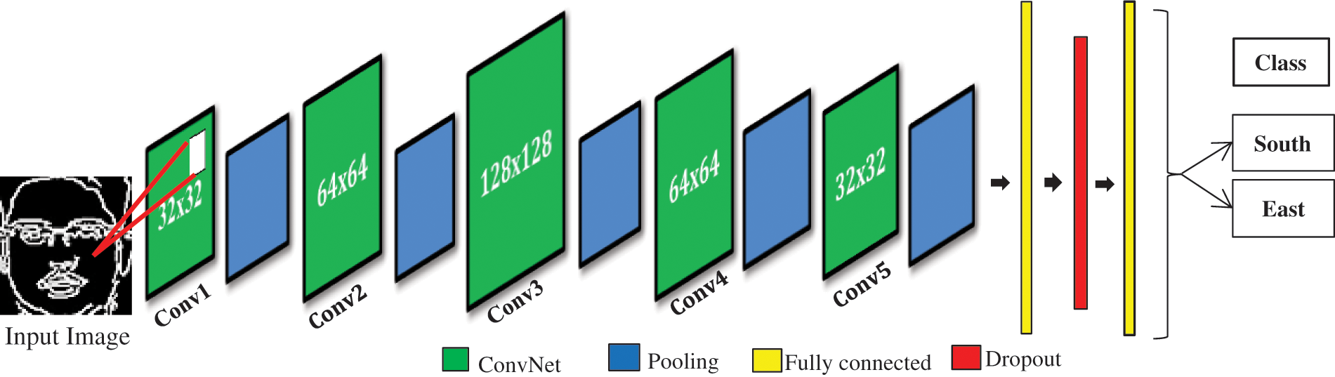
Figure 2: Constellation of CNN-FC architecture used to classify countered face images to region

Convolution Layers

In Fig. 2, the CNN-FC model has five convolutional layers. The first layer consists of 32 × 32 filters, the second layer of 64 × 64 filters, the third layer of 128 × 128 filters, the fourth layer of filter size 64 × 64, and the fifth layer of 32 × 32 filters. The traditional CNN has a fixed size of filters at different levels, and usually, filter size tends to decrease. Here we have used different filters of sizes 32 × 32, 64 × 64, then 128 × 128 with stride five, because filters are generally related to feature maps that will be flattened at the end to distinguish more shapes and textures. It is good practice to use filters of multiples of 2. It provides better RAM organization and batch size. At (m, n) location in the xth feature map of yth layer, zli, j, k, the feature value is calculated by Eq. (2).

Zm,n,yy=wxyTXm,ny+bxy (2)

where wxy and bxy are the weight vector and bias term of the xth filter of the yth layer, respectively and Xm,ny is the input patch cantered at location (m, n) of the yth layer.

ReLu (Rectified Linear Unit) Layers

CNN adapts to learn non-linear data. Most of the real-world data samples learned are primarily non-linear. Since the convolution layer is linear in operation, the ReLu layer helps convert the linear process to non-linear. ReLU transformation function f(x) is used to activate the nodes if the input (x) is above the threshold value, while if the input is below zero, then the output is zero. It showed a linear relationship with the dependent variable as in Eq. (3).

f(x)={0ifX<0XifX≥0 (3)

It has removed every –ve values from the filtered image and turns them to 0’s. Its non-saturation of gradient quality makes it a good choice in CNNs.

Pooling Layers

In this layer, we performed shift-variance by reducing the images obtained from the ReLu layer into a smaller size. After every layer, the feature map is halved without compromising the information. The feature map of each pooling layer is associated with the preceding layers corresponding feature map. Eq. (4) computes the pooling function pool (·) for each feature map.

ym,n,kl=pool(am,n,kl),∀(m,n)∈Ri,j (4)

where Ri, j represents a local neighborhood around (i, j) location. We have used 5 max pooling layers with 5 × 5 windows.

Fully Connected Layers

These are the final layers where the high-level reasoning takes place. The filtered and shrunken images are put in a single list. Two fully connected layers are used: one is of 1024 neurons, and the other is of 2 neurons.

Dropout Layer

This regularization technique is used for avoiding overfitting by preventing co-adaptations on Train_Set. A single dropout layer is added with a key probability of 0.8 (p = 0.8), followed by a dual-node decision layer. The output of this layer is denoted as in Eq. (5).

O=bv∗a(WZi) (5)

where i = [i1,i2,…,in]Z is considered input to fully-connected layer, W ∈ Mp×q denotes weight matrix, and bv represents a binary vector of size q being a Bernoulli distribution with parameter p, i.e., ri ∼ Bernoulli(p) as a source of every element. Finally, to reduce cross-entropy loss, the Adam optimizer is used with a learning rate α = 0.001.

This model is now trained with contoured face images obtained by the given algorithm.

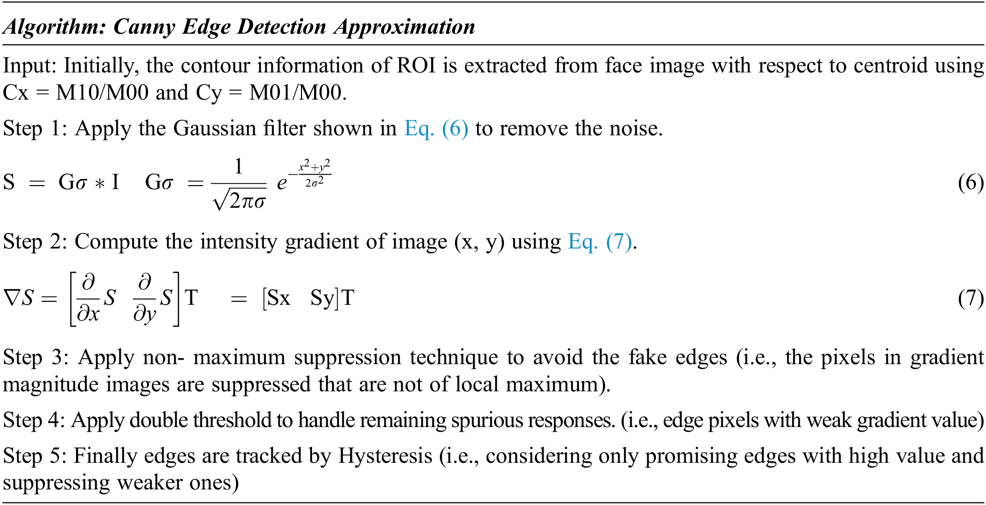
The contour approximation method ensured that all the image points were stored, keeping the original image intact.

3.3.3 M-CNN

Based on the empirical experiments, we have proposed variations to the CNN model by incorporating: The inception module, spectral pooling, and leaky ReLu activation function.

Inception Module

In conventional CNNs, convolution filter is a generalized linear model (GLM) representing the input image area. It is more suitable for the samples where abstract features are linearly separable. Here we propose an improved inception module to enhance its representation ability. These are used in CNN’s to reduce computational complexity and decrease the deeper network’s dimensionality with stacked 1 × 1 convolutions. Instead of having either 3 × 3 or 5 × 5 filters or a pooling layer, this model suggests having all of them. As shown in Fig. 3, the new architecture incorporates all 1 × 1, 3 × 3, 5 × 5 filters, and mixed pooling layers. The convolutional operation is performed on every output of the previous layer. The concatenated output from all filters passed as an input to the next layer. This process allowed the increase in depth and width of CNN without increasing the computational complexity.

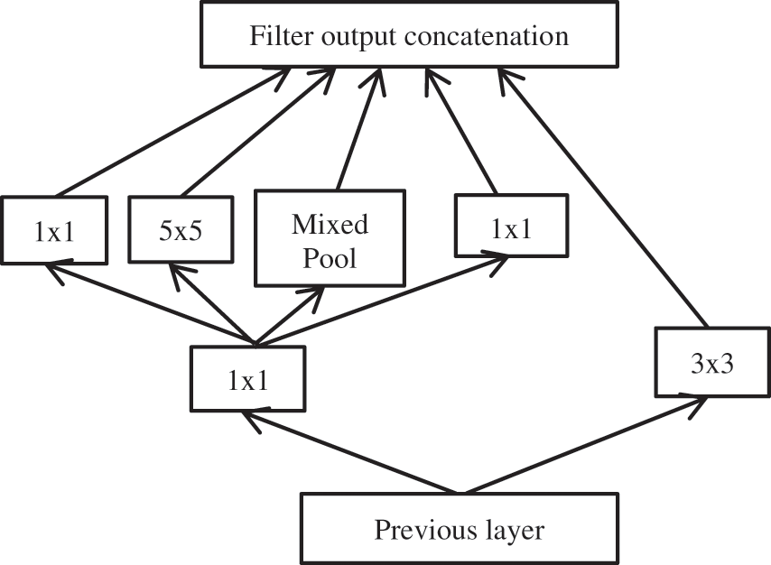
Figure 3: Improved inception model

In the first step, we have applied 128 filters of different sizes 1 × 1 and 3 × 3 on an input image. The feature map obtained from this step is fed to the second step so that all filters of different sizes 1 × 1,3 × 3 and 5 × 5 and mixed pooling should perform on the same image. Padding is kept identical to maintain the same output and input shape of Conv2D operation. So the outcome of each filter is the same. It helps in concatenating the output of each filter to get the output of the inception module. Such modules can solve the computational expense and overfitting issues.

Mixed Pooling

The function in Eq. (8) represents the mixed pooling technique. Here we have combined both max pooling and average pooling to have a better solution for the overfitting problem instead of applying alone of them.

Yi,j,k,=λ(m,n)€Ri,jmaxam,n,k+(1−λ)1|Ri,j|∑amn,k (8)

where λ = {0, 1} indicates the choice of max pooling or average pooling, respectively, the two-dimensional window runs over each channel of an input image, and a filter covers the features lying within the region. A feature map (FM) of dimension MxNxK gets a new size shown in Eq. (9) after the pooling layer.

FM=(M−f+1)sx(N−f+1)sxK (9)

where M and N are the height and width of the feature map, respectively, K is the number of channels, f is the size of the filter, and s is stride length.

Activation Function

A potential disadvantage of ReLU function Xm, n, k = max (ym, n, k, 0) found in CNN-FC is that the gradient turned to be zero whenever the unit was inactive. This disadvantage causes the problem of gradient-based optimization for weight adjustment. The training process is downturned because some idle units have never been active due to the persistent zero gradients. We incorporated leaky ReLu (Fig. 4) defined in Eq. (10) to alleviate this problem.

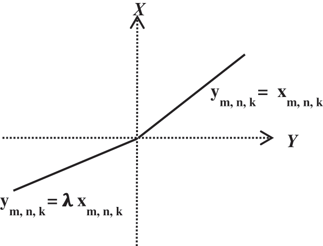
Figure 4: Leaky ReLu function, λ is default parameter value ranges between 0 and 1

Xm,n,k=max(ym,n,k,0)+λmin(ym,n,k,0) (10)

Unlike ReLU, the negative part in Leaky ReLU is compressed rather than mapping it to constant zero, which results in yielding a small and non-zero gradient while the unit is idle.

Loss Function Regularization and Optimizer

The underlying binary classification (where the number of classes C = 2) found that the cross-entropy loss shown in Eq. (11) is more suitable since it measures the classification model performance whose likelihood output value falls between 0 and 1.

Loss=∑i=12⁡yilogpi=−[ylog(p)+(1−y)log(1−p)] (11)

where yi is positive information ranging within 0 and 1 and pi is ith class Softmax probability. We have flattened the output to a 1-D array of neurons fed to two fully connected layers one is of 1024 neurons, and the other is of 2 neurons corresponding to two classes (decision layer). Overfitting occurred by preventing co-adaptations on Train_Set is reduced using the dropout regularization technique. A single dropout layer with 0.8 (p = 0.8) key probability is added, followed by a dual-node decision layer. Finally, the model is compiled with Adam optimizer to update weights iterative based in Train_Set with learning rate α = 0.001. The feature vector for each face consists of 1024 features.

4  Evaluation Metrics and Result Discussions

Development Environment

We have used Microsoft Windows 10 operating system as a primary system requirement with 2 GHz CPU processing speed and 4 GB of RAM. We installed Anaconda Navigator, an open-source distribution of python to implement computational models. The CNN and M-CNN models are developed in Spyder (the scientific python development environment. Additionally, we used TensorFlow with a GPU notebook provided by Google colaboratory on a Linux-based hosted machine.

4.1 Analysis of AHIS and MIS

We estimated the proficiency of identifiers rigorously on two Indian databases and compared the performance of computational models on the proposed database. The similar correlations are obtained for the two datasets (r = 0.68 ± 0.05 for Set 1, r = 0.61 ± 0.02 for Set 2; correlation in Set 1 > Set 2 in 885 of 1000 random samples). Set 1 and Set 2 have achieved 58% and 59.4% accuracy, respectively, based on assumptions made on regions. The main limitations with available relative databases are that they do not consist of region-wise labeled faces and are not adequate for supervised learning. The proposed database addresses this issue. The performances, including precision, recall, and F1 score of the proposed M-CNN model, are evaluated based on True Positive (TP), False Positive (FP), and False Negative (FN) metrics for the novel labeled dataset. All the metrics calculated are as follows:

Precision=TPTP+FP,Recall=TPTP+FN,F1=2∗precision∗recallprecision+recall

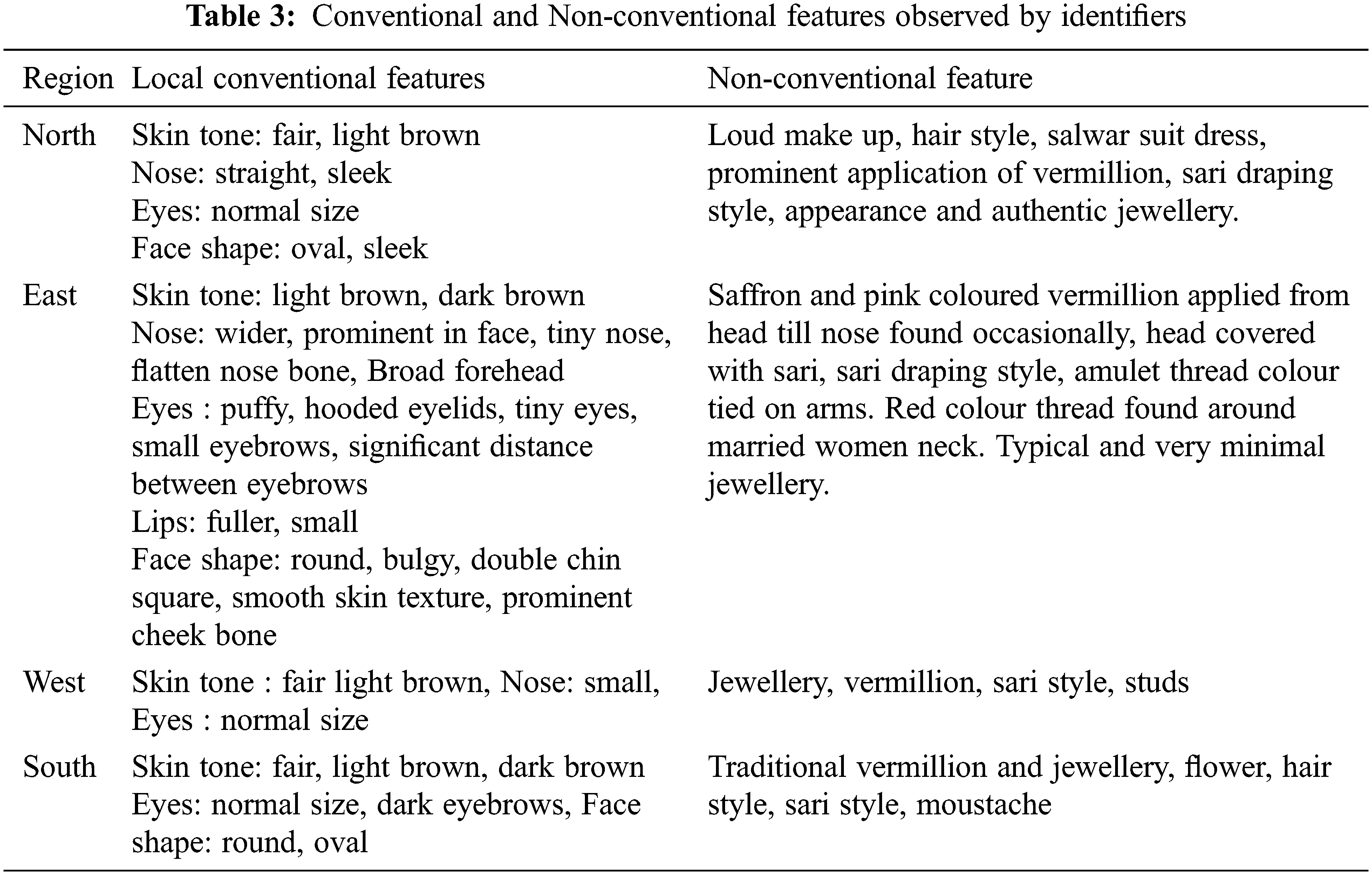
According to the Mann-Whitney U test, the probability of samples correctly classified from the South population is more remarkable than samples from the East population and is different (larger or smaller) than the probability of samples from the East exceeding the samples from the South; i.e., P (South > East) ≠ P (East > South) or P (South > East) + 0.5 · P (South = East) ≠ 0.5. Since the south region faces have more accurately classified (with correlation r = 79.5%) than the East (approximately r = 74.3%). The M-CNN model has shown a high stratified rate for shabby images (overall 77.9%) compared to a single featured based classifier and traditional CNN (61% and 65%, respectively). Tab. 3 presents a rich feature set drawn from the analysis of human visual response. It comprises both conventional and non-conventional facial features.

The accuracy of the proposed model is measured using the Genuine Acceptance Rate (GAR) and False Acceptance Rate (FAR) [28] performance evaluation metrics as stated in Eqs. (12) and (13) below:

GAR=CorrectlyclassifiedfacesTotalfaceimages×100% (12)

FAR=WronglyclassifiedfacesTotalfaceimages×100% (13)

4.2 Comparative Analysis of M-CNN against Conventional CNN using Statistical Hypothesis Test

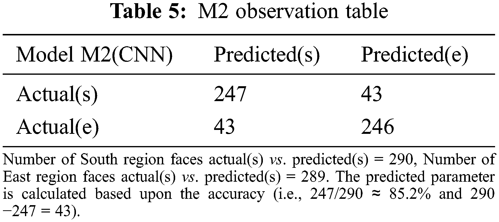
This section performed a comparative analysis based on the proposed Indian regional face dataset. The performance of the proposed M-CNN model against the conventional CNN model is measured using the Chi-Square statistical hypothesis testing. Let’s say M-CNN represents M1 and CNN is M2. Tabs. 4 and 5 presents the confusion matrixes of both M1 and M2.

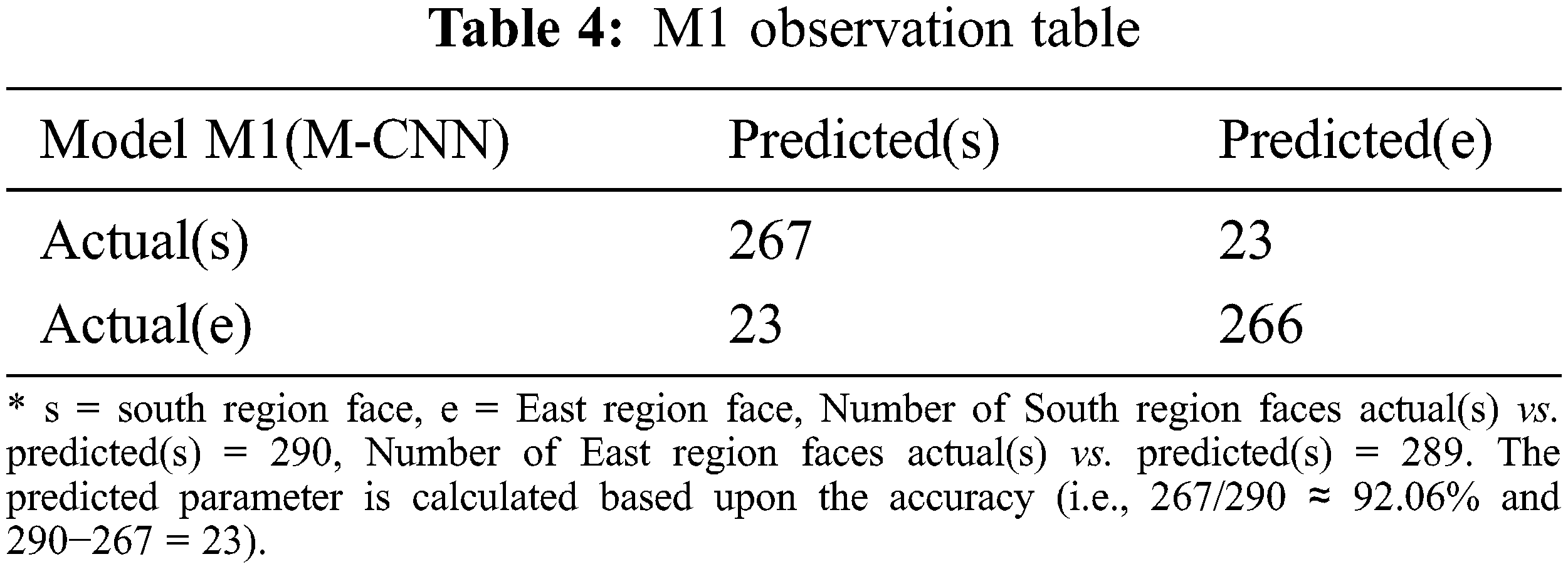
Chi-square test for evaluating M-CNN

According to the M1 observation table, the probability of data instances belonging to South is ± 92.06% and a ± 7.9% chance of East otherwise. In chi-square tests, we extract the expected values from observations. M1 (M-CNN) labels 290 instances as South. If M1 is randomly guessing, we can expect approx. 7.9% of those instances to be of East. Since there is 7.9%, the chances are that a test data instance is East. Hence according to the law of independent probability given in Eq. (14),

P(Predicted=sandActual=e)=P(Predicted=p)xP(Actual=a) (14)

We can derive the value of P (Predicted = s and Actual = e). P (Predicted = s) = 290/100 = 2.9

P(Predicted=sandActual=e)=2.9x0.079=0.23

So, 23% of the total data instances are likely to be classified as East face. Therefore, the number of East faces = 23% of 100 = 23. The following Fig. 5 shows the chi-square distribution with degree of freedom (DOF = 1).

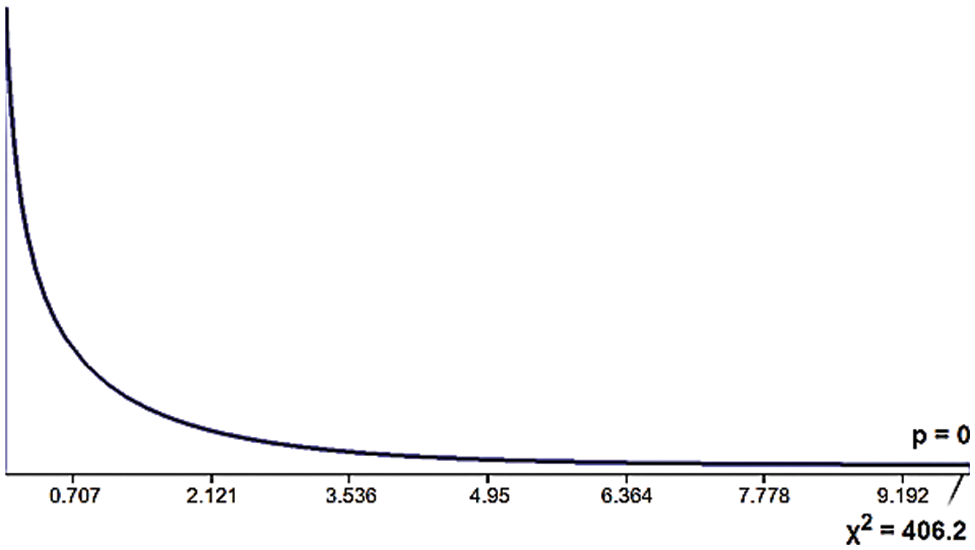
Figure 5: Chi-square distribution (DOF = 1) for Chi-square statistic = 406.26 P value = 2.4e-90

The chi-square distribution graph shows that the chi-square statistic is exceedingly high, and the probability (p-value) of a null hypothesis is insignificant compared to the alpha (0.05). Thus, we can claim that M1 is not a random predictor and better fits the data.

Comparing M-CNN against CNN using Matthew Correlation Coefficient (MCC)

We have used MCC statistics to evaluate the M1 and M2 models performance. Based upon the confusion matrices of M1 and M2 shown above, we have calculated the critical classification metrics such as 1.Accuracy (how suitable M1 is at prediction). 2. Sensitivity (how often M1 chooses the positive class when the observation is in the positive class). 3. Precision (how often an M1 is correct when it predicts the positive class). 4. Specificity (how often M1 chooses the negative class when the observation is a negative class). Tab. 6 presents the performance of M1 and M2 based on the metrics mentioned above.

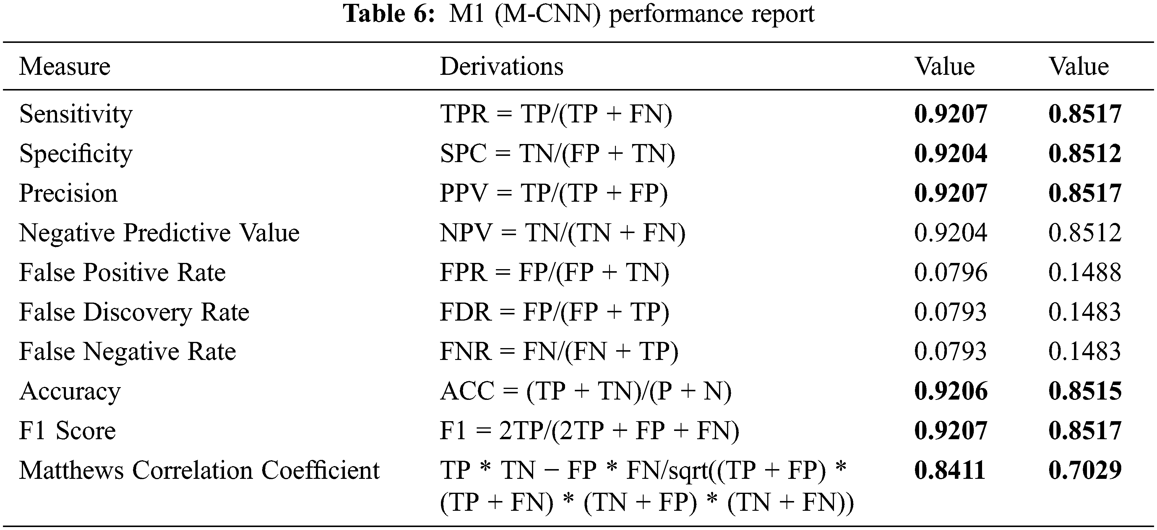
The recorded values against different metrics show that M1 significantly outperforms M2, the conventional CNN used in phase 3.3.2 in terms of accuracy, sensitivity, specificity, F1-score, and Matthew correlation coefficient. The Tensorboard graphs shown in Fig. 6 depict the accuracy and loss of model M1 (M-CNN). Fig. 6a chart shows the accuracy of 89.07% against the testing set. Fig. 6b shows the validation of the model as 92.98% against the training set. Fig. 6c demonstrates the cross-entropy loss estimation.

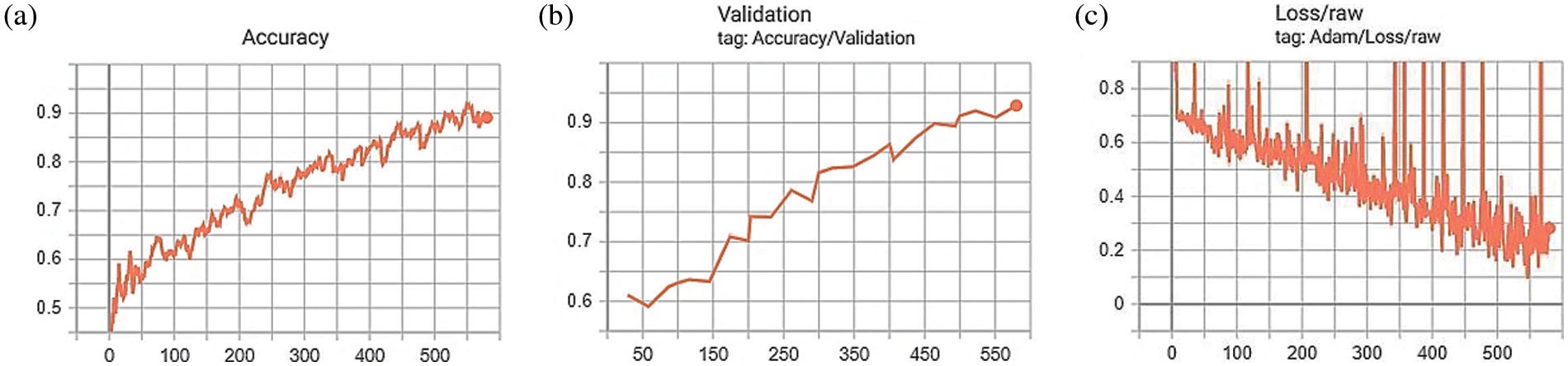
Figure 6: Visualization of feature mapping of training set images to testing image set using Tensorboard graphs. (a) Accuracy of model drawn from training the training set images with respect to image batch, (b) Validation of model with respect to testing image set and, (c) Loss by cross entropy

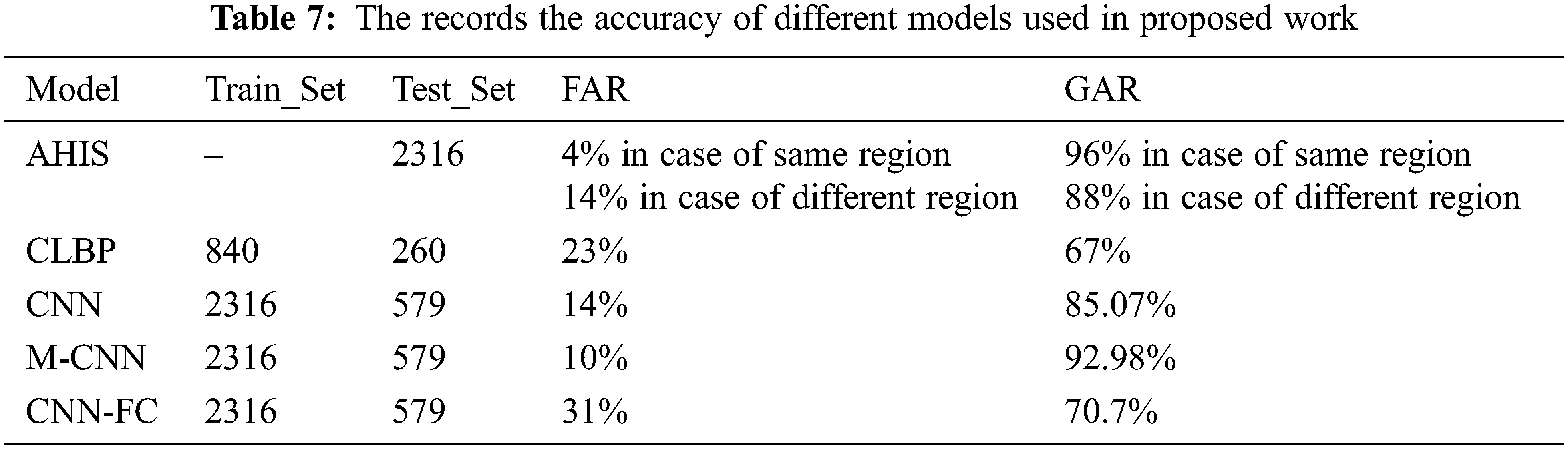
Tab. 7 presents the cumulative performance of human vision and the different computational models discussed in this work.

5  Conclusion

This research investigated human and machine intelligence performance under the Indian race classification problem involving human identifiers and computational models like CNN, M-CNN, CNN-FC, and CLBP. This work has shown the significance of customizing Deep Learning models for specific applications and projects. For intra-class face classification problems, the proposed M-CNN is highly recommended compared to the traditional CNN model. The CNN-FC model trained with contoured face images has characterized the influence of face shape among other facial features. This model would be prospected to explain the impact of face shape information. We have developed a novel Indian regional face database to mitigate the scarcity of labeled databases for underlying supervised classification problems. The experimental outcome showed the high proficiency of humans (96%) compared to machine vision algorithms (92.98%).

Acknowledgement: The authors acknowledge BIT Mesra, Ranchi for providing necessary tools and journal access in need. We are grateful to the renowned universities for providing help in data collection.

Funding Statement: The authors received no specific funding for this study.

Conflicts of Interest: The authors declare that they have no conflicts of interest to report regarding the present study.

This work is licensed under a Creative Commons Attribution 4.0 International License, which permits unrestricted use, distribution, and reproduction in any medium, provided the original work is properly cited.