DOI:10.32604/csse.2023.027647
| Computer Systems Science & Engineering DOI:10.32604/csse.2023.027647 | |
| Article |
Computer Vision and Deep Learning-enabled Weed Detection Model for Precision Agriculture
1Department of Information Technology, M.Kumarasamy College of Engineering, Karur, 639113, India
2Department of Computer Science and Engineering, K. Ramakrishnan College of Technology, Tiruchirapalli, 621112, India
3Department of Electronics and Instrumentation, Easwari Engineering College, Tamil Nadu, 600089, India
4Pondicherry University, Puducherry, 605014, India
5Department of computer science and engineering, The Oxford college of Engineering, Bangalore, 560068, India
6Department of Computer Science Engineering, Saveetha School of Engineering, Saveetha Institute of Medical and Technical Sciences, Saveetha University, Chennai, 602105, India
7Department of Computer and Information Science, Faculty of Science, Annamalai University Chidambaram, 608002, India
*Corresponding Author: S. P. Balamurugan. Email: spbcdm@gmail.com
Received: 22 January 2022; Accepted: 06 March 2022
Abstract: Presently, precision agriculture processes like plant disease, crop yield prediction, species recognition, weed detection, and irrigation can be accomplished by the use of computer vision (CV) approaches. Weed plays a vital role in influencing crop productivity. The wastage and pollution of farmland's natural atmosphere instigated by full coverage chemical herbicide spraying are increased. Since the proper identification of weeds from crops helps to reduce the usage of herbicide and improve productivity, this study presents a novel computer vision and deep learning based weed detection and classification (CVDL-WDC) model for precision agriculture. The proposed CVDL-WDC technique intends to properly discriminate the plants as well as weeds. The proposed CVDL-WDC technique involves two processes namely multiscale Faster RCNN based object detection and optimal extreme learning machine (ELM) based weed classification. The parameters of the ELM model are optimally adjusted by the use of farmland fertility optimization (FFO) algorithm. A comprehensive simulation analysis of the CVDL-WDC technique against benchmark dataset reported the enhanced outcomes over its recent approaches interms of several measures.
Keywords: Precision agriculture; smart farming; weed detection; computer vision; deep learning
Presently, several smart agriculture tasks, namely crop yield prediction, plant disease detection, weed detection, water and soil conservation, and species identification, are comprehended by using computer vision (CV) technique [1]. Weed control is a significant method for improving crop production [2]. Significant research has presented accurate variable spraying methods to avoid herbicide residual issues and waste created by the conventional full coverage spraying [3]. To accomplish accurate variable spraying, the main problem that needs to be resolved is how to understand realtime accurate recognition and classification of weeds crops [4]. In traditional agriculture settings, herbicide is employed at uniform rate to the entire field although distribution of weed is patchy. It causes environmental pollution and leads to higher input costs for farmers [5]. In contradiction of this, Precision Agriculture (PA) purposes necessity-based on site-specific application [6].
Adapting PA practice for using herbicides needs precise weed mapping by categorizing host plants and weeds [7]. Classification of plants is a tedious process due to spectral resemblances among distinct kinds of plants. The current mapping method assumes that host plant is planted in rows. The line detection approach is utilized for categorizing plants in a row as host plant, and plant that falls out of seeding line as weeds. The interline method failed to identify weed plants positioned inside crop lines and host plant falls out of crop line [8]. Method to realize weed recognition through CV technique primarily consist of deep learning and conventional image processing. Once weed recognition is implemented by using conventional image-processing technique, feature extraction, namely color, shape, and texture, of the image and combined with conventional machine learning (ML) approaches like Support Vector Machine (SVM) or random forest, for weed detection is needed [9]. This method needs to develop features automatically and have higher dependence on image acquisition method, pre-processing method, and the quality of feature extraction. Due to the development in computing power and the growth in data dimensions, DL approaches could extract multi-scale and multi-dimensional spatial semantic feature data of weeds by using Convolution Neural Network (CNN) because of improved data expression capability, avoiding the drawbacks of conventional extraction method. Hence, they have received growing interest towards the authors [10].
Lottes et al. presented a novel crop-weed classification model which depends on fully convolutional networks (FCN) with encoding-decoding infrastructure and incorporates spatial data with assuming image sequence [11]. The exploitation the crop arrangement data that is noticeable in the image orders allows this technique for robustly estimating pixel-wise labeling of images as to crop and weed, for instance, a semantic segmentation. The RGB color images of seedling rice are taken from paddy fields, and ground truth (GT) images are attained by manually labeling the pixel from the RGB image with 3 distinct types such as weed, rice seedling, and background [12]. The class weight co-efficient is computed for solving the problem of unbalance of the amount of classification type. The GT as well as RGB
A software is established, Pynovisão that with utilize of superpixel segmentation technique SLIC is utilized for building a robust image data set and classify image utilizing the method training by Caffe software [13]. For comparing the outcomes of ConvNets, SVMs, AdaBoost, and RF are utilized in conjunction with group of shape, color, and texture feature extracting approaches. A novel method is developed which combined different shape features for establishing a pattern for all varieties of plants. For enabling the vision system from the detection of weeds dependent upon its patterns, SVM and ANN are utilized [14]. Four species of general weed from sugar beet field are considered. The shape feature fixed contained Fourier descriptors and moment invariant feature. Pereira et al. [15] presented the automatic identification of any species using techniques of supervised pattern detection approach and shape descriptor for composing an adjacent future expert method to automatic application of correct herbicide. The experimentally utilizing several recent approaches have demonstrated the robustness of utilized pattern detection approaches.
The major contributions of the study are discussed as follows. This study presents a novel computer vision and deep learning based weed detection and classification (CVDL-WDC) model for precision agriculture. The proposed CVDL-WDC technique intends to properly discriminate the plants as well as weeds. The proposed CVDL-WDC technique involves two processes namely multiscale Faster RCNN based object detection and optimal extreme learning machine (ELM) based weed classification. The parameters of the ELM model are optimally adjusted by the use of farmland fertility optimization (FFO) algorithm. A comprehensive simulation analysis of the CVDL-WDC technique against benchmark dataset and the results are examined under diverse dimensions.
The rest of the study is organized as follows. Section 2 elaborates the working of CVDL-WDC technique and the experimental results are offered in Section 3. Lastly, Section 4 concludes the study.
This study has developed a new CVDL-WDC technique for proper discrimination of plants and weeds in precision agriculture. The proposed CVDL-WDC technique encompasses a series of subprocesses namely WF based pre-processing, Multi-scale Faster RCNN based object detection, ELM based classification, and FFO based parameter optimization. The proposed model properly identified the weeds among crops, reduce the usage of herbicide and improve productivity. Fig. 1 illustrates the overall prcoess of CVDL-WDC technique.
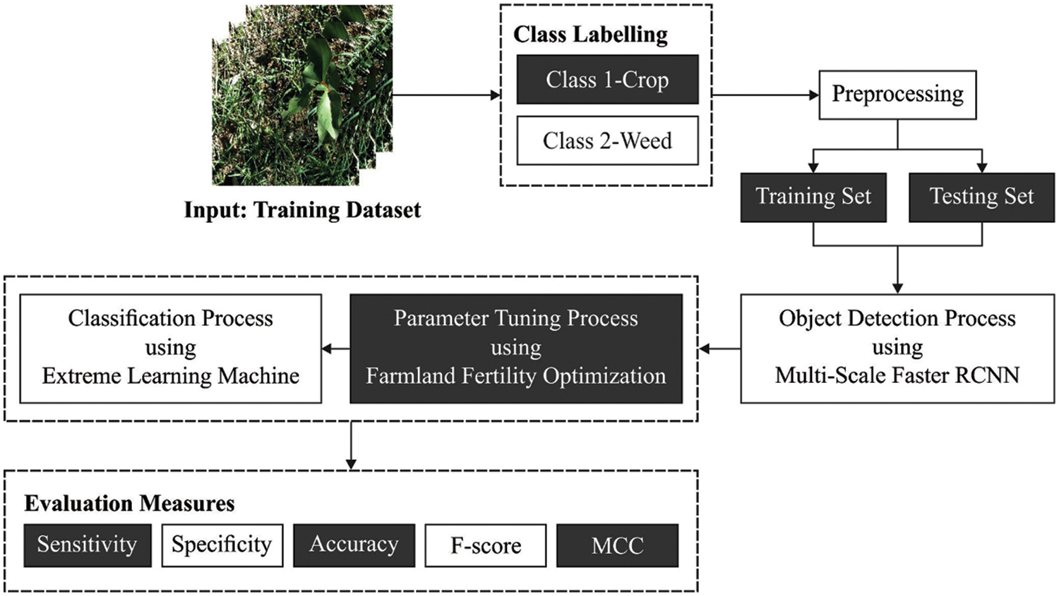
Figure 1: Overall process of CVDL-WDC technique
2.1 Pre-processing Using WF Technique
At the initial stage, the WF approach can be utilized for eradicating the noise that exists in the image. Noise removal is an image pre-processing approach proposed to optimize the feature of the image corrupted by noise [16]. A certain instance is adoptive filtering whereby the denoising is typically performed according to the noise content existing in the image. Consider the corrupted image is described as
when the noise variance through the image is equivalent to zero,
When
2.2 Multiscale Faster RCNN Based Object Detection
During object detection process, the multiscale Faster RCNN model is applied to identify the weeds as well as plants. Indeed, the recognized object is smaller in size and lower in resolution. The earlier models (i.e., Fast RCNN) has better recognition performance for larger objects cannot efficiently identify smaller object in an image [17]. The primary reason is that this model depends on DNN which makes the image evaluated with downsampled and convolution for obtaining high-level and more abstract features. Every downsampling causes the image to be minimized by half. When the object is analogous to the size of object in the PASCAL VOC, the object detailed feature is attained by using this downsampling and convolution. But, When the recognized object is on a smaller scale, the last feature might be left 1-2 pixels afterward several downsampling. Consequently, some characteristics could not completely determine the features of the object and the current recognition technique could not efficiently identify the smaller target object. The deep the convolutional process, the more abstract the object feature could denote the higher-level feature of object. The shallow convolutional layer extracts the lower-level feature of object. However, for smaller objects, the lower-level feature ensures effective object features. For getting higher-level and abstract object features and ensuring that there is sufficient pixel to determine smaller objects, we combined the feature of distinct scales for ensuring the local detail of the object. Simultaneously, focus more interest on the global features of the object depending upon the Fast RCNN.
The multiscale Faster RCNN method is separated into four portions: the initial one is the feature extraction that contains 2 pooling layers, 3
Whereas X represents the original vector from , , and layers,
Whereas
2.3 Optimal ELM Based Weed Classification
At the time of weed classification, the features are received by the ELM to classify into distinct classes. Huang et al. presented ELM for improving the network trained speed, afterward extensive the concept of ELM in neuron hidden node to another hidden node [18]. The trained instances are signified as
where
where
Usually, orthogonal projection is utilized for solving the generalization inverse
In order to boost the classification efficiency of the ELM model, the FFO algorithm is applied to it. A metaheuristic is a type of model-free method to resolve different kinds of optimization issues which are newly exploited in a wide-ranging application. The FFO approach involves six major portions which are described below [19]:
1. Initialization: here, the possible solution and the number of sections for (n) in the farmland are determined. Regarding, the population (N) is modeled by the following equation:
Whereas
Whereas,
2. Evaluate the quality of soil in each section of the farmland: this phase directs the farmland decision variable in the section. Calculate the cost function values for the decision variable. Likewise, the soil quality was attained as follows:
3. Update the memory: here, the local and global memories are upgraded. The optimal solution of the farmland is saved in the local memory and the solutions amongst them are taken into account as global memory. For determining the amount of optimum local and global memories, the subsequent formulas are utilized:
Whereas,
4. Soil quality difference for all the sections: define the quality of section and store the optimal one in the local memory. Moreover, the optimal solution is saved in the global memory. To improve the worst-case result, they are upgraded by integrating to the optimal-case solution of global memory. At last, the variable of the solution is upgraded by:
In the equation,
in which,
while
5. The composition of soil: afterward detecting the optimal local solution
In which,
6. Last condition: compute the potential solution to the searching region. In the method, once the ending condition is attained, the procedure stops, or else, it is repeated until attaining the optimal solution. FFO algorithm derives a fitness function to attain improved classification performance. It determines a positive integer to represent the better performance of the candidate solutions. In this study, the minimization of the classification error rate is considered as the fitness function, as given in Eq. (22). The optimal solution has a minimal error rate and the worse solution attains an increased error rate.
This section examines the weed detection and classification results of the CVDL-WDC technique using the benchmark dataset [20]. Fig. 2 demonstrates the sample images consisting of healthy plants as well as weeds. Fig. 3 illustrates the visualization result analysis of the CVDL-WDC technique. The figure stated that the CVDL-WDC technique has effectively recognized and classified weeds among other plants.
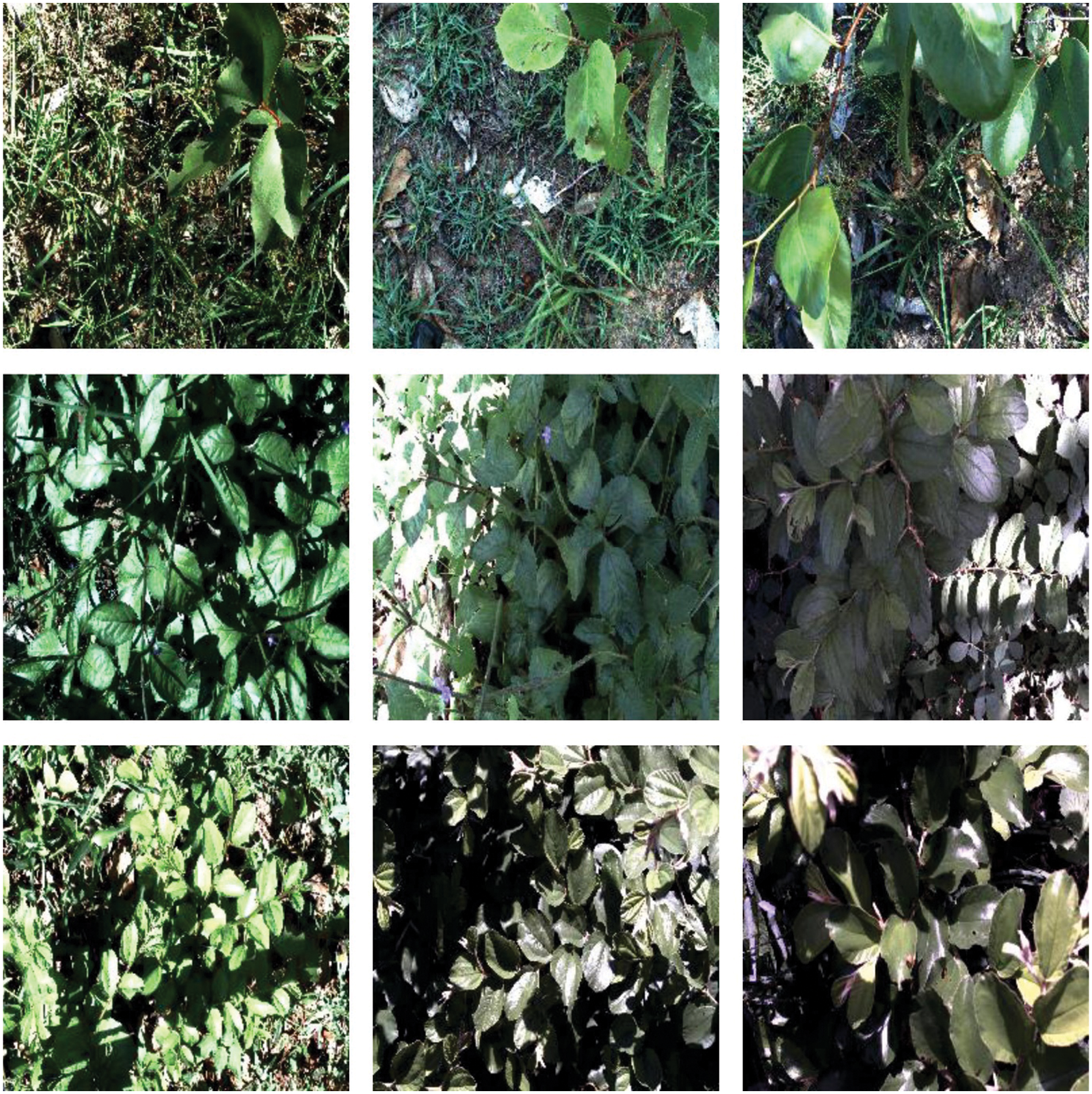
Figure 2: Sample images
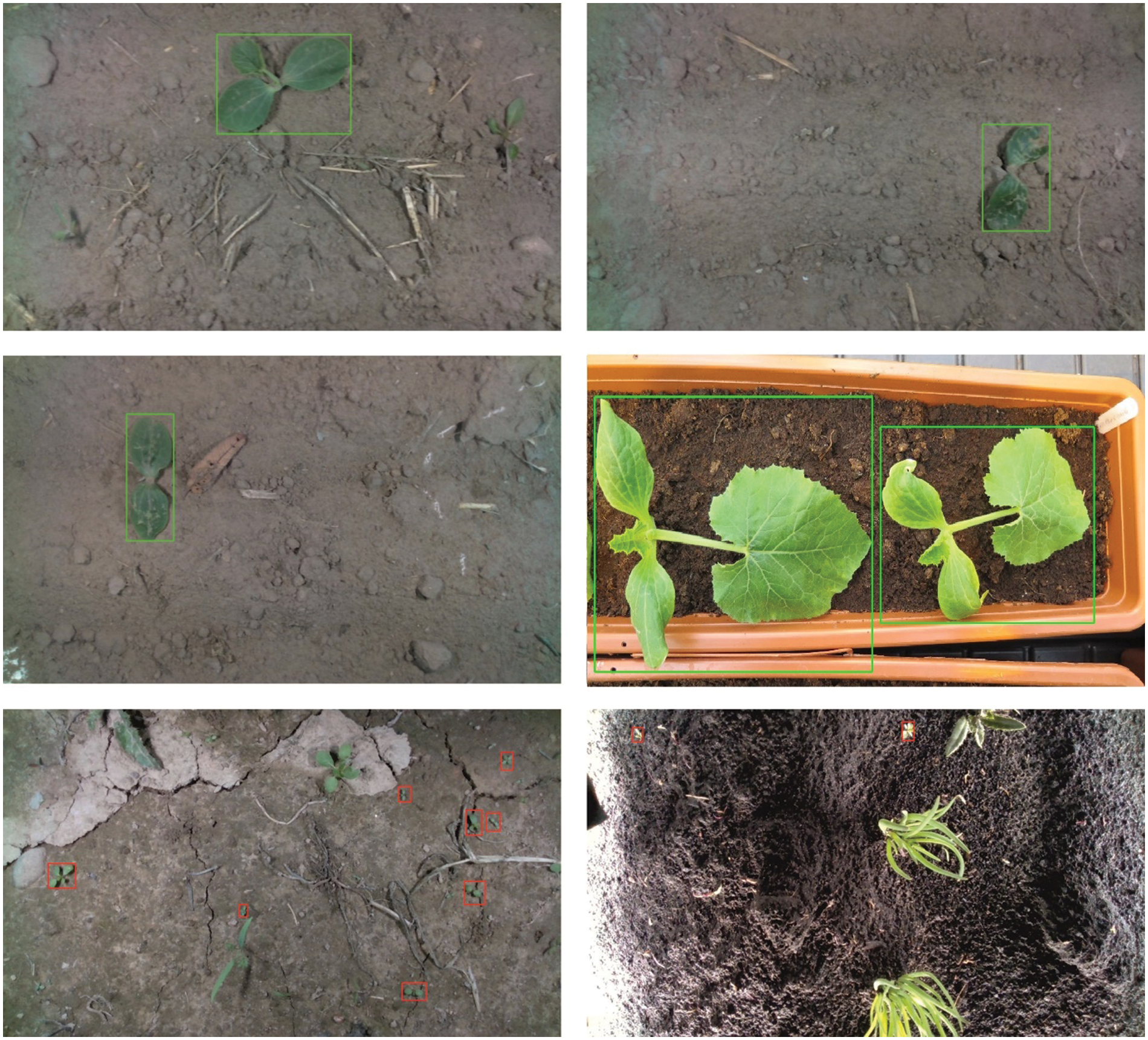
Figure 3: Annotated images-crop indicated in green box weed indicated in red box
Tab. 1 and Fig. 4 offers a brief classification result analysis of the CVDL-WDC technique under distinct sizes of training/testing data. The results indicated that the CVDL-WDC technique has the ability to attain improved classifier results under all sizes of training/testing data. With training/testing data of 80:20, the CVDL-WDC technique has offered
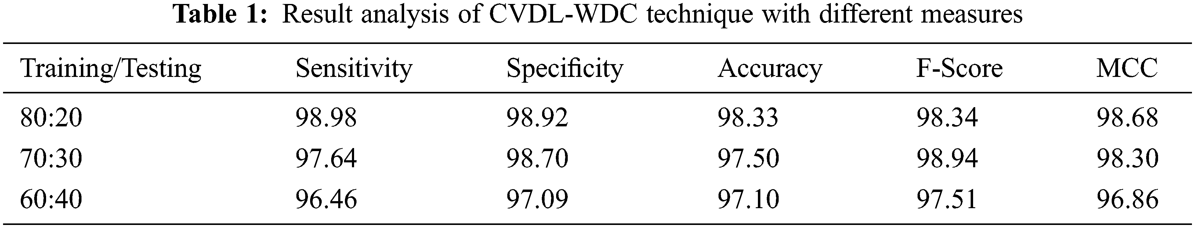

Figure 4: Result analysis of CVDL-WDC technique with different measures
Fig. 5 offers the accuracy and loss graph analysis of the CVDL-WDC approach on the test dataset. The outcomes demonstrated that the accuracy value tends to increase and loss value tends to reduce with an increase in epoch count. It is also observed that the training loss is low and validation accuracy is maximum on the test dataset.

Figure 5: Accuracy and loss analysis of CVDL-WDC technique
Tab. 2 offers a detailed comparative study of the CVDL-WDC technique with recent methods. Fig. 6 illustrates the comparative
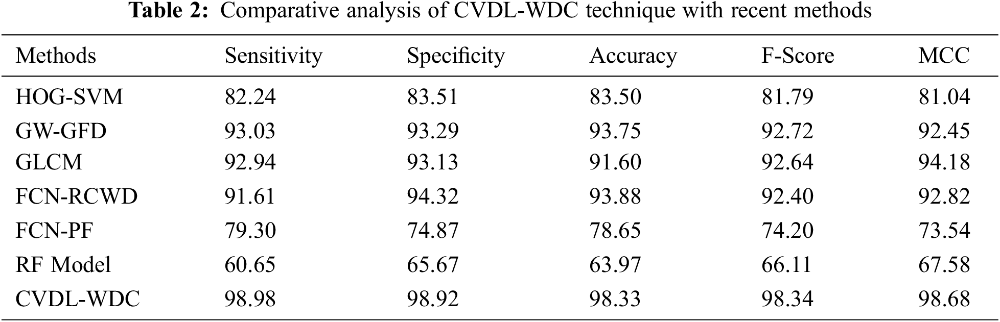

Figure 6:
Fig. 7 depicts the comparative

Figure 7:
Fig. 8 showcases the comparative

Figure 8:
Fig. 9 portrays the comparative

Figure 9:
Fig. 10 demonstrates the detailed

Figure 10: MCC analysis of CVDL-WDC technique with recent approaches
Lastly, a comprehensive computational time (CT) analysis of the CVDL-WDC technique takes place in Tab. 3 and Fig. 11 [21]. The results show that the HOG-SVM and GW-GFD techniques have required increased CT of 235 and 205 s respectively. Along with that, the GLCM, FCN-PF, and RF techniques have needed slightly decreased CT of 185, 137, and 156 s respectively. In line with, the FCN-RCWD technique has accomplished somewhat considerable CT of 78 s. However, the proposed CVDL-WDC technique has attained minimal CT of 43 s. From the results and discussion, it is evident that the CVDL-WDC technique has reached effective weed detection and classification performance.
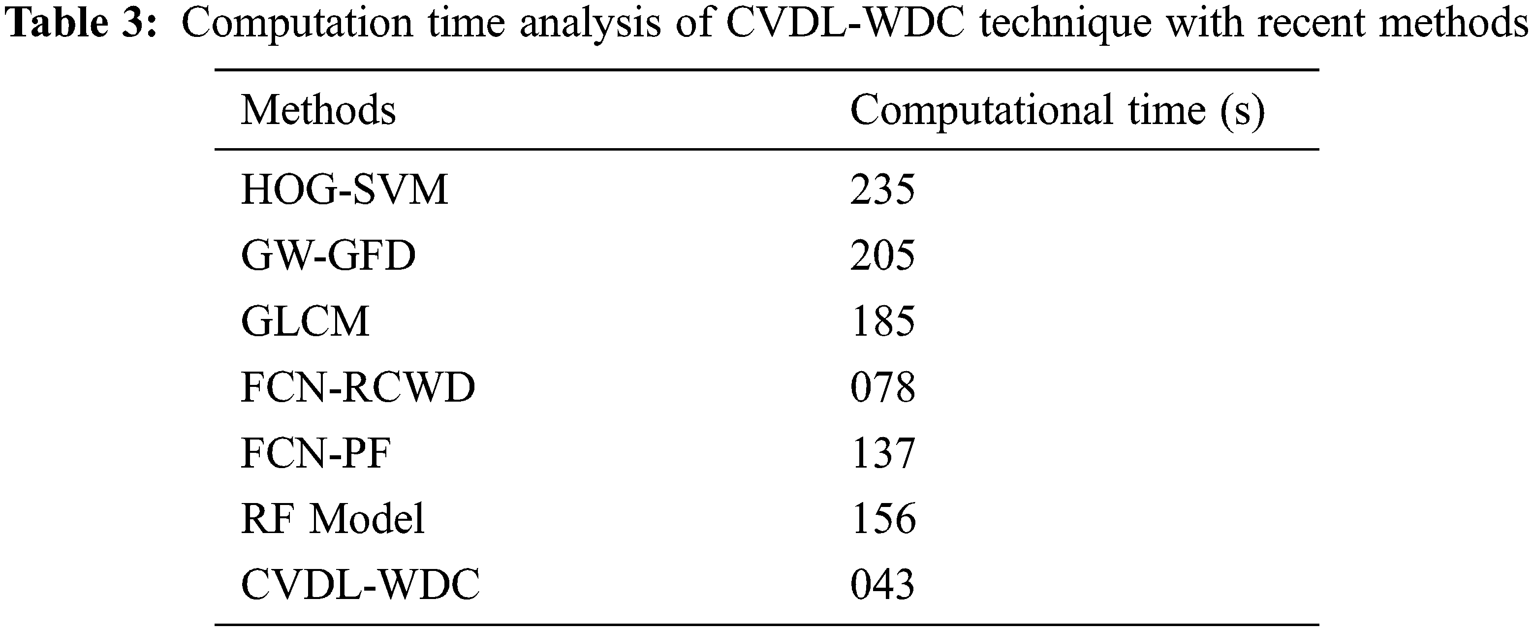

Figure 11: CT analysis of CVDL-WDC technique with recent methods
This study has developed a new CVDL-WDC technique for proper discrimination of plants and weeds on precision agriculture. The proposed CVDL-WDC technique encompasses a series of subprocesses namely WF based pre-processing, Multi-scale Faster RCNN based object detection, ELM based classification, and FFO based parameter optimization. The proposed model properly identified the weeds among crops, reduce the usage of herbicide and improve productivity. A comprehensive simulation analysis of the CVDL-WDC technique against benchmark dataset and the results are examined under diverse dimensions. The comparative results reported the enhanced outcomes over its recent approaches interms of several measures. As a part of future extension, the proposed CVDL-WDC technique can be utilized in the Internet of Things and smartphone environment.
Funding Statement: The authors received no specific funding for this study.
Conflicts of Interest: The authors declare that they have no conflicts of interest to report regarding the present study.
1. R. Kamath, M. Balachandra and S. Prabhu, “Paddy crop and weed discrimination: A multiple classifier system approach,” International Journal of Agronomy, vol. 2020, no. 3 and 4, pp. 1–14, 2020. [Google Scholar]
2. B. Liu and R. Bruch, “Weed detection for selective spraying: A review,” Current Robotics Reports, vol. 1, no. 1, pp. 19–26, 2020. [Google Scholar]
3. H. Huang, Y. Lan, J. Deng, A. Yang, X. Deng et al., “A semantic labeling approach for accurate weed mapping of high resolution UAV imagery,” Sensors, vol. 18, no. 7, pp. 2113, 2018. [Google Scholar]
4. N. Islam, M. M. Rashid, S. Wibowo, C. Y. Xu, A. Morshed et al., “Early weed detection using image processing and machine learning techniques in an Australian CHILLI FARM,” Agriculture, vol. 11, no. 5, pp. 387, 2021. [Google Scholar]
5. J. Yu, S. M. Sharpe, A. W. Schumann and N. S. Boyd, “Deep learning for image-based weed detection in turfgrass,” European Journal of Agronomy, vol. 104, pp. 78–84, 2019. [Google Scholar]
6. A. Wang, W. Zhang and X. Wei, “A review on weed detection using ground-based machine vision and image processing techniques,” Computers and Electronics in Agriculture, vol. 158, pp. 226–240, 2019. [Google Scholar]
7. J. Yu, A. W. Schumann, Z. Cao, S. M. Sharpe and N. S. Boyd, “Weed detection in perennial ryegrass with deep learning convolutional neural network,” Frontiers in Plant Science, vol. 10, pp. 1422, 2019. [Google Scholar]
8. A. N. Veeranampalayam Sivakumar, J. Li, S. Scott, E. Psota, A. Jhala et al., “Comparison of object detection and patch-based classification deep learning models on mid- to late-season weed detection in UAV imagery,” Remote Sensing, vol. 12, no. 13, pp. 2136, 2020. [Google Scholar]
9. A. Kamilaris and F. Prenafeta-Boldú, “Deep learning in agriculture: A survey,” Computers and Electronics in Agriculture, vol. 147, no. 2, pp. 70–90, 2018. [Google Scholar]
10. K. Hu, G. Coleman, S. Zeng, Z. Wang and M. Walsh, “Graph weeds net: A graph-based deep learning method for weed recognition,” Computers and Electronics in Agriculture, vol. 174, no. 7, pp. 105520, 2020. [Google Scholar]
11. P. Lottes, J. Behley, A. Milioto and C. Stachniss, “Fully convolutional networks with sequential information for robust crop and weed detection in precision farming,” IEEE Robotics and Automation Letters, vol. 3, no. 4, pp. 2870–2877, 2018. [Google Scholar]
12. X. Ma, X. Deng, L. Qi, Y. Jiang, H. Li et al., “Fully convolutional network for rice seedling and weed image segmentation at the seedling stage in paddy fields,” PLoS ONE, vol. 14, no. 4, pp. e0215676, 2019. [Google Scholar]
13. A. dos Santos Ferreira, D. Matte Freitas, G. Gonçalves da Silva, H. Pistori and M. Theophilo Folhes, “Weed detection in soybean crops using ConvNets,” Computers and Electronics in Agriculture, vol. 143, no. 11, pp. 314–324, 2017. [Google Scholar]
14. A. Bakhshipour and A. Jafari, “Evaluation of support vector machine and artificial neural networks in weed detection using shape features,” Computers and Electronics in Agriculture, vol. 145, pp. 153–160, 2018. [Google Scholar]
15. L. Pereira, R. Nakamura, G. de Souza, D. Martins and J. Papa, “Aquatic weed automatic classification using machine learning techniques,” Computers and Electronics in Agriculture, vol. 87, no. 1, pp. 56–63, 2012. [Google Scholar]
16. J. Chen, J. Benesty, Y. Huang and S. Doclo, “New insights into the noise reduction Wiener filter,” IEEE Transactions on Audio, Speech, and Language Processing, vol. 14, no. 4, pp. 1218–1234, 2006. [Google Scholar]
17. G. X. Hu, Z. Yang, L. Hu, L. Huang and J. M. Han, “Small object detection with multiscale features,” International Journal of Digital Multimedia Broadcasting, vol. 2018, no. 2, pp. 1–10, 2018. [Google Scholar]
18. G-B. Huang, Q-Y. Zhu and C-K. Siew, “Extreme learning machine: Theory and applications,” Neurocomputing, vol. 70, no. 1–3, pp. 489–501, 2006. [Google Scholar]
19. H. Shayanfar and F. S. Gharehchopogh, “Farmland fertility: A new metaheuristic algorithm for solving continuous optimization problems,” Applied Soft Computing, vol. 71, no. 4, pp. 728–746, 2018. [Google Scholar]
20. K. Sudars, J. Jasko, I. Namatevs, L. Ozola and N. Badaukis, “Dataset of annotated food crops and weed images for robotic computer vision control,” Data in Brief, vol. 31, no. 1, pp. 105833, 2020. [Google Scholar]
21. Z. Wu, Y. Chen, B. Zhao, X. Kang and Y. Ding, “Review of weed detection methods based on computer vision,” Sensors, vol. 21, no. 11, pp. 3647, 2021. [Google Scholar]
 | This work is licensed under a Creative Commons Attribution 4.0 International License, which permits unrestricted use, distribution, and reproduction in any medium, provided the original work is properly cited. |