Computer Systems Science & Engineering DOI:10.32604/csse.2023.028107
Article

Optimal Machine Learning Enabled Performance Monitoring for Learning Management Systems

Ashit Kumar Dutta1,*, Mazen Mushabab Alqahtani2, Yasser Albagory3, Abdul Rahaman Wahab Sait4 and Majed Alsanea5

1Department of Computer Science and Information Systems, College of Applied Sciences, AlMaarefa University, Ad Diriyah, 13713, Riyadh, Kingdom of Saudi Arabia
2Physical Therapy Department, Majmaah University, Majmaah, 11952, Kingdom of Saudi Arabia
3Department of Computer Engineering, College of Computers and Information Technology, Taif University, Taif, 21944, Kingdom of Saudi Arabia
4Department of Archives and Communication, King Faisal University, Al Ahsa, 31982, Hofuf, Kingdom of Saudi Arabia
5Department of Computing, Arabeast Colleges, Riyadh, 11583, Kingdom of Saudi Arabia
*Corresponding Author: Ashit Kumar Dutta. Email: adotta@mcst.edu.sa
Received: 02 February 2022; Accepted: 30 March 2022

Abstract: Learning Management System (LMS) is an application software that is used in automation, delivery, administration, tracking, and reporting of courses and programs in educational sector. The LMS which exploits machine learning (ML) has the ability of accessing user data and exploit it for improving the learning experience. The recently developed artificial intelligence (AI) and ML models helps to accomplish effective performance monitoring for LMS. Among the different processes involved in ML based LMS, feature selection and classification processes find beneficial. In this motivation, this study introduces Glowworm-based Feature Selection with Machine Learning Enabled Performance Monitoring (GSO-MFWELM) technique for LMS. The key objective of the proposed GSO-MFWELM technique is to effectually monitor the performance in LMS. The proposed GSO-MFWELM technique involves GSO-based feature selection technique to select the optimal features. Besides, Weighted Extreme Learning Machine (WELM) model is applied for classification process whereas the parameters involved in WELM model are optimally fine-tuned with the help of Mayfly Optimization (MFO) algorithm. The design of GSO and MFO techniques result in reduced computation complexity and improved classification performance. The presented GSO-MFWELM technique was validated for its performance against benchmark dataset and the results were inspected under several aspects. The simulation results established the supremacy of GSO-MFWELM technique over recent approaches with the maximum classification accuracy of 0.9589.

Keywords: Learning management system; data mining; performance monitoring; machine learning; feature selection

1  Introduction

Nowadays, education techniques have been increasingly adopted in higher education institutions since teaching is no longer limited to Face-to-Face (F2F) physically-interactive sessions [1]. For university courses, the integration of F2F teaching and e-learning increases the flexibility, choices, and accessibility for communication [2]. This achievement in instructional productivity is made possible by Learning Management System (LMS) that is commonly employed as the environment to support e-learning and hybrid online F2F courses. This advanced LMS has the potential to accomplish conventional instructional activities through online such as course material management, dissemination of information, evaluation and collection of students’ feedback. After the outbreak of COVID-19, universities have increasingly adopted LMS to support the course [3]. Education Data Mining (EDM) is an emerging field that is concerned with emergent techniques to evaluate distinct types of information acquired from educational setting. This technique is also used to develop the settings where both faculty and student share knowledge [4]. EDM is a multi-disciplinary research domain that investigates statistical modeling, Data Mining (DM), and Artificial Intelligence (AI) with information generated from education institution [5]. Fig. 1 shows the objectives of an LMS.

Figure 1: Goals in learning management system

EDM uses computational method to handle education data in order to investigate the educational queries as its final goal [6]. In order to make a country stand exclusive among other countries worldwide, the education system needs to have knowledge as a principal progression which can be achieved through improving the learning pedagogy from time to time. The hidden pattern in the data, collected from various information sources, is extracted by adopting DM method. In order to summarize the performance of students with their credentials, the researchers checked how DM can be exploited in educational field. Each educational institute generates huge volumes of information every year. New information is transferred considerably when using DM method. The information accomplished from educational institutes undergo inspection with the help of distinct DM models [7]. The technique detects the environment, where a student gets better inspiration to lead a useful life [8]. Weka, an efficient DM model was proposed earlier and utilized to generate substantial outcomes. The drastic growth of educational information [9] from heterogeneous sources results in an urgent need for EDM study. This could help in achieving the objectives so as to determine some educational purposes. In Machine Learning (ML) with increasing dimensions of the data, there is an increasing number of information required to provide a reliable analysis. Feature subset selection works by removing irrelevant or redundant features. The subset of features selected should follow Occam Razor principle so that it can offer important outcome. In some instances, NP remains a challenging issue and is resolved by metaheuristic approach [10].

The aim of the study conducted by Ahmmed et al. [11] is to carry out student visa processing via ML. The ML technique can be implemented at the place where the visas get rejected or approved for higher studies abroad. In this study, the researchers predicted the visa information for higher studies on the basis of student’s background information. Next, the information is processed (through transformation, cleaning, standardization, feature selection, and integration). Then, various classifier techniques were used such as k-nearest neighbor (KNN), C4.5 (j48), random forest (RF), naïve bayes (NB), neural network (NN), and support vector machine (SVM), to classify the model. Hung et al. [12] employed EDM to explore the learning behavior of students in blended learning courses through the data collected from them. The experiment information was gathered from first-year students enrolled in Python programming courses at a university located in north Taiwan. During a semester, high-risk learners might be forecasted precisely by the data produced from blended education platform. In literature [13], the researchers presented a method to predict the student’s dropout with NB Classifier method in R language. The study also investigated the reasons for students drop out at an earlier stage. The model forecasted whether a student may drop out or not in future. This study cited many factors that affect a student to drop out from the course.

Sarra et al. [14] estimated the helpfulness of a certain class method i.e., Bayesian Profile Regression, for identification of students who are likely to drop out from their courses. Students’ resilience, performance, and motivation were considered and the method allowed to draw a student’s profile with high risks of educational failure. In literature [15], EDM method with KNN and Multilayer Perceptron (MLP) approaches are used to predict the performance of the learner. The classifier outcomes were satisfactory while the kNN classification attained the optimal outcomes. The experiment outcome shows that the performance of the learner can be evaluated. Further, the researchers observed a relationship between learning performance and video sequence viewing behavior. Ramaswami et al. [16] established a generic prediction method that can identify at-risk students over a wide range of courses. The experiment was implemented by a variety of approaches and when generic method was used, it produced an efficient outcome. It was found to be an outstanding candidate to provide solutions in this field, given the fact that it can flawlessly manage missing and categorical information.

In this background, the current study introduces a Glowworm based Feature Selection with Machine Learning Enabled Performance Monitoring (GSO-MFWELM) technique for LMS. The major intention of the proposed GSO-MFWELM technique is to effectively monitor the performance in LMS. GSO-MFWELM technique primarily designs a GSO-based Feature Selection (FS) technique to select the optimal features. Besides, a Weighted Extreme Learning Machine (WELM) model is applied for classification process whereas the parameters involved in WELM model are optimally fine-tuned with the help of Mayfly Optimization (MFO) algorithm. GSO-MFWELM technique was validated for its performance against benchmark dataset and the results were inspected under several aspects.

2  The Proposed Model

In current study, a new GSO-MFWELM technique has been developed to monitor the performance of LMS. The proposed GSO-MFWELM technique encompasses three major processes namely, feature subset selection, WELM-based classification, and MFO-based parameter tuning. The weight values of WELM model can be optimally elected by MFO algorithm with classification error rate as the objective function. Fig. 2 illustrates the working process of GSO-MFWELM technique.

Figure 2: Overall process of GSO-MFWELM technique

2.1 Steps Involved in GSO-FS Technique

In this stage, the learning data is fed into GSO-FS technique to elect an optimal subset of features. GSO [17] is a smart optimization technique that functions according to the phenomenon in which the light, emitted by glowworm, is utilized as a signal to attract glowworms. This approach includes a collection of glowworms that are arbitrarily distributed. All the glowworms are considered to be potential solutions, characterized by their location. The glowworm, with high luminosity, exhibits high brightness and so it attracts glowworms with low-brightness. In this manner, global optimization is accomplished. The elementary steps are as follows.

Step 1. Initialize the elementary parameter of GSO. This parameter includes fluorescein update rate γ, population size g, fluorescein volatilization factor ρ, set of glowworms Ni(t) in the decision domain, update rate β of the dynamic decision domain, perception radius rs, move step s and threshold nt for the number of glowworms in the neighborhood.

Step 2. The fitness value of glowworm i during tth iteration is transformed into fluorescein value as given herewith.

li(t)=(1−ρ)li(t−1)+γJ(X(t)) (1)

where as ρ represents the fluorescein decay constant that belongs to (0, 1) and γ indicates the fluorescein enhancement constant.

Step 3. All the glowworms select individuals with high brightness than the dynamic decision radius rdi(t) to form the neighbor set Ni(t).

Step 4. Evaluate the probability pij(t) of glowworm Xi(t) that moves towards the glowworm Xj(t) in a dynamic decision radius as follows.

pij(t)=lj(t)−li(t)∑k∈Ni(t)⁡lk(t)−li(t) (2)

Step 5. Upgrade the location of glowworm X(t) as follows

Xi(t+1)=Xi(t)+s×[Xj(t)−Xi(t)||Xj(t)−Xi(t)||] (3)

Step 6. Upgrade the dynamic decision radius of glowworm X(t) as follows.

rdi(t+1)={minrs,{max0,β×(nt−|Ni(t)|)}} (4)

The arithmetical formula of FS is presented. In general, the classification (that is., supervised learning) of data sets sized NS × NF is performed whereas NF denotes the amount of features and NS represents the amount of samples. The primary goal of FS is to choose a subset of features S from the overall amount of features (NF) in which the size of S is lesser, when compared to NF. It is attained by minimizing the subsequent objective function.

Fit=λ×γS+(1−λ)×(|S|NF) (5)

Here γS represents the classification error that use S whereas |S| indicates the number of selected features.

λ is utilized for balancing between (|S|NP) and γS.

2.2 WELM Based Classification

During classification process, WELM model is applied for the classification of learning data. WELM is an extended version of Extreme Learning Machine (ELM) [18]. With mapped data set χi′,yj∈ℜp×ℜc(i=1,2,…,n) , the outcome of generalization in Single Layer Feed Forward Networks (SLFN) with q hidden node and activation function h(x′) are properly written as follows

oi=∑k=1q⁡βkhk(χi′)=∑k=1q⁡βkh(wk,bk,xi′), (6)

where i=1,2,…,n,wk=[wk1,wk2,…,wkp]T refers to input weight vector that links the input node and kth hidden node, bk refers to the bias of kth hidden node, βk=[βk1,βk2,…,βkc]T signifies the resultant weight vector that links the resultant node and kth hidden node, and 0i refers to the predictable output of ith sample. The activation function generally utilized from ELM contains multiquadric, sigmoid, hard limit, and Gaussian RBF functions. Eq. (6) is equivalently modified as follows.

Hβ=O, (7)

where H defines the hidden state resultant matrix of SLFNs and is determined as follows.

H=H(w1,…,wq,b1,…,bq,x1′,…,xn′)=[h(x1′)⋮h(xn′)] (8)

=[h(w1,b1,x1′)⋯h(wq,bq,x1′)⋮⋱⋮h(w1,b1,x1′)⋯h(wq,bq,x1′)]n×q

where the ith row of H refers to the resultant vector of hidden state, in terms of input sample xi′ , and the kth column of H refers to the resultant vector of kth hidden node in terms of input instances x1′,x2′,...,xn′ . β implies weight matrix that links the hidden as well as output layers which are determined as follows

β=[β1T⋮βqT]q×c (9)

O stands for the predictable label matrix while all the rows signify the resultant vector of one instance. O is determined as given herewith.

O=[o1T⋮TOn]=[o11⋯01c⋮⋱⋮on1⋯0nc] (10)

While the target of trained SLFN is to minimize the outcome error, for instance, similar to the input instances with zero error as below.

∑i=1n⁡‖0i−yi‖=‖O−Y‖=0 (11)

where y=[y1T⋮Tyn]=[y11⋯y1c⋮⋱⋮yn1⋯ync] represents the target resultant matrix.

Hβ=Y (12)

In ELM, the weight wk of input connection and bias bk of hidden state nodes are arbitrarily and individually selected. Once this parameter is allocated, Eq. (12) is changed to suit the linear system and the resultant weight matrix β is logically defined as finding the least-square solutions of linear system.

minβ⁡‖Hβ−Y‖ (13)

An optimum solution of Eq. (13) as:

β^=H†Y=(HTH) (14)

where H† demonstrates Moore-Penrose generalization inverse of the hidden state resultant matrix, H. Here, β^ is made sure to be a less trained error and optimum generalized capability is obtained herewith. Further, it also avoids plunging the local optimally since β^ is unique. At last, it takes the classifier function of ELM as follows.

f(x′)=h(x′)β^=h(x′)H†y (15)

If ELM classifier is constructed, it can be determined a n × n diagonal matrix W, in which the diagonal element Wii refers to the weight of the trained instance χi′ . In particular, when χi′ appears to a majority class, the weight Wii is comparatively lesser than the instance that appears to minority class. Based on the KKT statement, Eq. (14) is modified as follows.

β^=H†Y=(HTWH)−1HTWT (16)

Afterward, Eq. (15) is developed as follows.

f(x′)=h(x′)β^=h(x′)(HTWH)−1HTWT (17)

Mostly, there are two structures exist to assign the weights to instances of two classes as follows.

W1=Wii={1/nPifxi′∈minorityclass1/nNifxi′∈majorityclass (18)

or

W2=Wii={0.618/nPifxi′∈minorityclass1/nNifxi′∈majorityclass, (19)

where Wl and W2 refere to two weighting processes, nP and nN signify the amount of samples of minority as well as majority classes correspondingly.

2.3 MFO Based Parameter Optimization

Finally, MFO algorithm is employed to fine tune the parameters of WELM technique, thereby enhancing the classifier results. The recently-designed MFO is an alteration of the familiar Particle Swarm Optimization (PSO) [19]. Since it is a combination of strength found in different optimization methods, it is assumed as a hybrid model. MFO algorithm is inspired by the social behavior of mayflies. Mayflies form as adults while the fittest one survives. Initially, two groups of population are created such as male and female populations. The candidate is characterized as a d-dimension vector x = (x1, …, xd). Then, the fitness of the candidate is estimated by the fitness function, f(x). The velocity v = (v1, …, vd) represents the change in candidate position. All the candidates modify their trajectory based on their optimal position (pbest) and the optimal position of each mayfly (gbest) [20].

The congregation of male mayfly reflects the experience of all the males in defining its position, regarding the neighborsI location. In order to determine xit as the existing position of candidate solution i at time t, the location can be modified by adding a velocity vit+1

xit+1=xit+vit+1 (20)

With xi0U(xmin,xmax) .

Assume the lower velocity of the male population while the velocity is estimated as follows

vijt+1=vijt+a1e−βrp2(pbestij−xijt)+a2e−βrg2(gbesti−xijt) (21)

Here, vijt represents the velocity of mayfly i,xijt denotes the location of mayfly i, a1 and a2 are determined as positive constants that represent the attraction. pbesti denotes the optimal position achieved by the candidate solution i, and pbestij at the subsequent phase while t + 1 is defined as follows.

pbesti={xit+1,iff(xit+1)<f(pbesti)sameasbefore,otherwise (22)

Whereas f:ℝn ⇒ ℝ denotes the function to be minimalized, gbest indicates the global optimal position reached for the problem ever, at time t. The coefficient in Eq. (21) limits a populationIs visibility. rp characterizes the distance between xi and pbesti. In the meantime, rg describes the distance from xi to gbest. rp and rg are defined as follows.

‖xi−Xi‖=∑j=1n⁡(xij−Xij)2 (23)

Whereas xij represents the jth element of ith candidate. Xi is correlated to pbest.

The optimal fit candidate keeps implanting up and down movement by varied velocity. The velocity is defined as follows.

vijt+1=vijt+d∗r (24)

Here d represents a coefficient correlated to up and down movements and r indicates a random value between − 1 and 1.

Female mayfly does not gather, but tend to move towards the male mayflies. Here, yit is defined as the existing position of female mayfly i at time t.

yit+1=yit+vit+1 (25)

with yi0 U (xmin,xmax) .

The velocity of the female mayfly is defined as follows.

vijt+1={vijt+a2e−βrmf2(xijt−yijt),iff(yi)>f(xi)vijt+fl∗r,iff(yi)≤f(xi) (26)

Here, vijt indicates the velocity of ith female at time t,yijt shows the position of ith female candidate solution at time t, a2 represent a positive constant, β denotes a fixed coefficient, rmf symbolizes the distance among the male candidates’ solutions and the female one is calculated by Eq. (23), fl denotes a coefficient that corresponds to the female which remains unattracted, and r implies an arbitrary value between − 1 and 1.

Mating can be denoted by the operator i.e., crossover operator. A couple of male and female mayfly parents is selected. Next, the crossover operator creates two offspring as follows.

offspringl=L∗male+(1−L)∗female

offspring2=L∗female+(1−L)∗male (27)

Here, L represents an arbitrary value. At first, the velocity of offspring is equal to zero.

3  Experimental Validation

The proposed model was validated for its performance against benchmark dataset from UCI repository (available at https://archive.ics.uci.edu/ml/datasets/student+performance). The dataset includes 649 samples with 33 attributes under two classes. Class 0 (pass) includes 549 samples, whereas class 1 (fail) includes 100 instances.

Fig. 3 shows the correlation matrix generated for the test dataset. Tab. 1 shows the feature selection results of Chaotic Whale Optimization Algorithm (CWOA)-FS and GSO-FS techniques. The results show the outcomes of GSO-FS technique since it selected 15 features, whereas the presented CWOA-FS technique selected 20 features out of 32 and established its supremacy.

Figure 3: Correlation matrix of the proposed method

Fig. 4 demonstrates the confusion matrices generated by the proposed GSO-MFWELM technique under various Hidden Units (HUs). With HU-1, GSO-MFWELM technique categorized 529 instances under class 0 and 94 instances under class 1. Eventually, with HU-3, the proposed GSO-MFWELM approach categorized 531 instances under class 0 and 93 instances under class 1. Meanwhile, with HU-6, the presented GSO-MFWELM system categorized 528 instances under class 0 and 93 instances under class 1. The values in the confusion matrix are tabulated in Tab. 2 in terms of True Positive (TP), True Negative (TN), False Positive (FP), and False Negative (FN).

Figure 4: Confusion matrix of GSO-MFWELM technique under various HUs

Tab. 3 offers the classification results of the analysis accomplished by GSO-MFWELM technique under distinct Hidden Units (HUs).

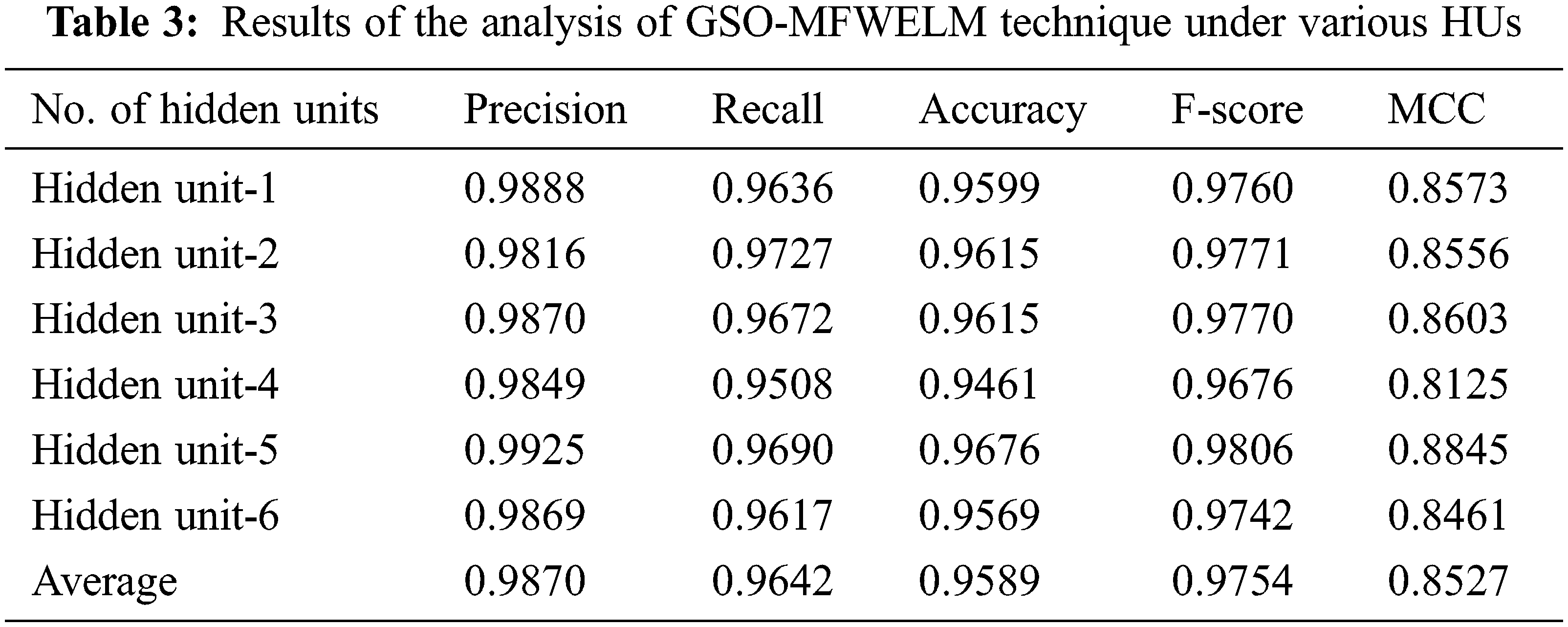
Fig. 5 shows the results of precn, recal, and accuy analysis attained by GSO-MFWELM technique under different HUs. The experimental values indicate that the proposed GSO-MFWELM technique obtained effectual classification performance. For instance, with HU-1, GSO-MFWELM technique attained precn, recal, and accuy values such as 0.9888, 0.9636, and 0.9599 respectively. In addition to this, with HU-6, GSO-MFWELM approach reached precn, recal, and accuy values namely, 0.9869, 0.9617, and 0.9569.

Figure 5: Results of the analysis of GSO-MFWELM technique under various HUs

Fig. 6 offers the Fscore and Mathew Correlation Coefficient (MCC) analysis results accomplished by GSO-MFWELM technique under various HUs. The experimental values point out the effectual classification performance of GSO-MFWELM technique. For instance, with HU-1, the proposed GSO-MFWELM technique obtained Fscore and MCC values such as 0.9760 and 0.8573 correspondingly. Besides, with HU-6, the proposed GSO-MFWELM technique achieved Fscore and MCC values namely, 0.9742 and 0.8461.

Figure 6: F-score and MCC analysis results of GSO-MFWELM technique under various HUs

Fig. 7 portrays the average analysis results achieved by the proposed GSO-MFWELM technique under distinct HUs. The figure infers that the proposed GSO-MFWELM technique achieved average precn of 0.9870, recal of 0.9642, accuy of 0.9589, Fscore of 0.9754, and MCC of 0.8527.

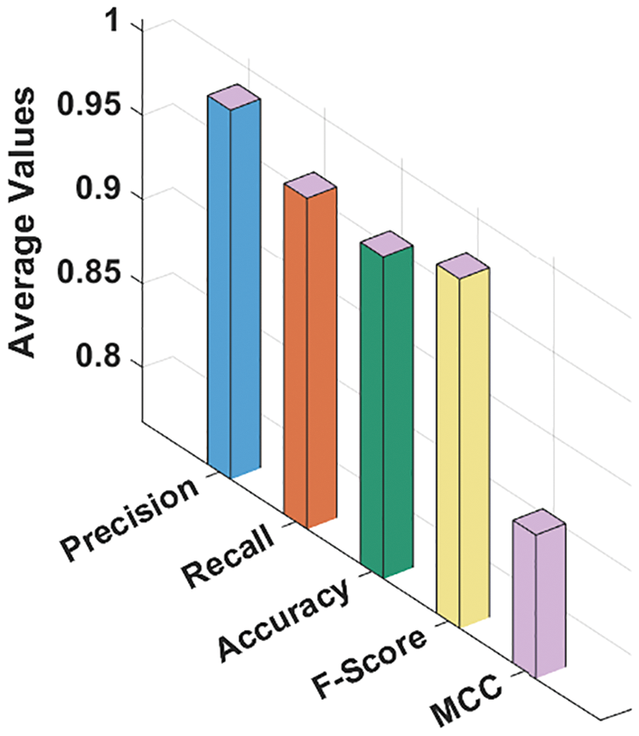
Figure 7: Average analysis results of GSO-MFWELM technique with distinct measures

Fig. 8 demonstrates the analysis results of GSO-MFWELM system against recent approaches in terms of precn and recal. The results illustrate that NN and SVM methods achieved minimal precn and recal values. Besides, Decision Tree (DT) and Random Forest (RF) techniques obtained certainly increased values in terms of precn and recal. Furthermore, mproved Evolutionary Algorithm based Feature Subset Selection with Neuro Fuzzy Classifier (IEAFSS-NFC) and Neural fuzzy classifier (FC) techniques obtained reasonable precn and recal values. At last, the proposed GSO-MFWELM methodology surpassed all other techniques and achieved precn and recal values such as 0.9870 and 0.9642.

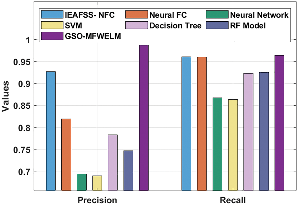
Figure 8: Precn and Recal analysis results of GSO-MFWELM technique with recent approaches

Fig. 9 showcases the results of the analysis of GSO-MFWELM technique against recent methods in terms of accuy. The results show that both NN and SVM models achieved the least accuy values. At the same time, DT and RF models achieved certainly increased values of accuy. Moreover, IEAFSS-NFC and Neural FC techniques obtained reasonable accuy values. However, the proposed GSO-MFWELM technique surpassed all other methods and achieved an accuy of 0.9589.

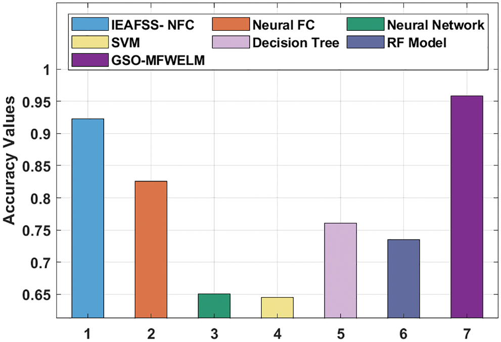
Figure 9: Accy analysis results of GSO-MFWELM technique with recent approaches

Tab. 4 highlights the comparison results of GSO-MFWELM technique against existing models [21].

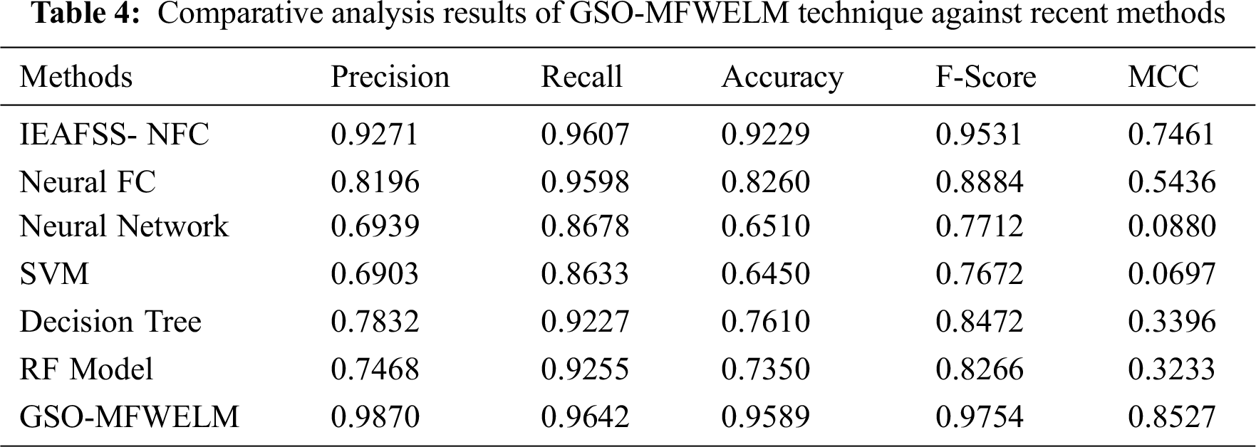
Fig. 10 depicts the results achieved by GSO-MFWELM algorithm in analysis against recent methodologies with respect to Fscore and MCC. The results infer that NN and SVM models obtained the least Fscore and MCC values. Simultaneously, DT and RF approaches reached certainly increased Fscore and MCC values. In addition, IEAFSS-NFC and Neural FC methods achieved reasonable Fscore and MCC values. Finally, the proposed GSO-MFWELM algorithm surpassed all other methods with the highest Fscore and MCC values such as 0.9754 and 0.8527. Therefore, it has been established from the above discussed results that the proposed model has the ability to attain maximum results over existing techniques.

Figure 10: Fscore and MCC analysis results of GSO-MFWELM technique with recent approaches

4  Conclusion

In current study, a new GSO-MFWELM technique has been developed to monitor LMS performance. The proposed GSO-MFWELM technique encompasses three major processes namely, feature subset selection, WELM based-classification, and MFO-based parameter tuning. The weight values of the WELM model can be optimally elected by MFO algorithm with classification error rate as an objective function. The proposed GSO-MFWELM technique was validated for performance using benchmark dataset and the results were inspected under several aspects. The simulation results infer the supremacy of the proposed GSO-MFWELM technique over recent approaches under different measures. In future, clustering techniques can be integrated into GSO-MFWELM technique to achieve enhanced performance.

Acknowledgement: The authors deeply acknowledge the Researchers supporting program (TUMA-Project-2021-27) Almaarefa University, Riyadh, Saudi Arabia for supporting steps of this work.

Funding Statement: This research was supported by the Researchers Supporting Program (TUMA-Project-2021-27) Almaarefa University, Riyadh, Saudi Arabia. Taif University Researchers Supporting Project number (TURSP-2020/161), Taif University, Taif, Saudi Arabia.

Conflicts of Interest: The authors declare that they have no conflicts of interest to report regarding the present study.

This work is licensed under a Creative Commons Attribution 4.0 International License, which permits unrestricted use, distribution, and reproduction in any medium, provided the original work is properly cited.