DOI: 10.32604/EE.2021.013239
ARTICLE
An Advanced Approach for Improving the Prediction Accuracy of Natural Gas Price
1School of Economics and Management, Nanjing University of Science and Technology, Nanjing, China
2School of Business, Nanjing Normal University, Nanjing, China
*Corresponding Author: Fanyi Meng. Email: tsyz-mengfanyi@163.com
Received: 30 July 2020; Accepted: 10 September 2020
Abstract: As one of the most important commodity futures, the price forecasting of natural gas futures is of great significance for hedging and risk aversion. This paper mainly focuses on natural gas futures pricing which considers seasonality fluctuations. In order to study this issue, we propose a modified approach called six-factor model, in which the influence of seasonal fluctuations are eliminated in every random factor. Using Monte Carlo method, we first assess and comparative analyze the fitting ability of three-factor model and six-factor model for the out of sample data. It is found that six-factor model has better performance than three-factor model and natural gas futures prices is strongly influenced by winter effect. We then apply the proposed model to predict the price of natural gas futures in the year 2019. It is found that natural gas prices have a weak upward trend in the coming year and are relatively volatile in winter.
Keywords: Natural gas futures; price forecasting; six-factor model; Monte Carlo method; seasonality
Commodity futures are taking increasingly important place in the world derivatives market. Natural gas is one of the most vital commodity futures, its trading volume ranks second in energy futures, only behind oil. Natural gas is mainly used as fuel, and accounts for a quarter of the residential daily fuel consumptions in the United States. Recently, the technical progress on shale gas also promotes the development of natural gas.
As a clean energy, natural gas is playing an important role in the transition from traditional energy to low-carbon energy. The development of natural gas has stimulated the investment demand for natural gas futures from investors and risk hedgers. Therefore, price forecasting of natural gas futures is of great significance for investment decision making. However, this topic has not got much concern in the literature. Previous studies often focus on the pricing issues of the general commodity futures.
The research on commodity futures pricing derives from the topic on general financial derivatives. Before the 1980s, scholars generally believed that the price of the underlying asset was the only stochastic factor for the pricing of financial derivatives. When pricing commodity futures, it was generally considered spot price was the only uncertainty, which is one-factor model. Until Brennan [1] first pointed out the significance of convenience yield in futures pricing, more factors began to be considered to add into commodity pricing models. Gibson et al. [2] proposed a well-known two-factor model in the study of crude oil futures. Spot price and convenience yield are two stochastic factors for crude oil futures pricing. The model was later widely used to study the pricing of general commodity futures. Subsequently, Schwartz [3] proposed a three-factor model and applied it to the pricing of crude oil, gold and copper futures. The model added a stochastic risk-free interest rate based on the two-factor model. Miltersen et al. [4] made further developments on the three-factor model.
Many subsequent studies have focused on investigating the impact of random convenience returns or the jump diffusion process of commodity prices. For example, Casassus et al. [5] regarded convenience yield as a dependence of spot price and risk-free interest rate, and proposed a three-factor model that considered time-varying risk premium. Liu et al. [6] modeled the volatility of the convenience yield related to its level, and the pricing problem of commodity futures was reconsidered. In addition to providing a convenient rate of return, there are some documents that add a mechanism conversion framework to the pricing model. The underlying idea of this framework is that one or more stochastic factors in the model are not in a state balance, but randomly switch in several regimes. One-factor regime switching model was proposed by Chen and Forsyth [7], in which the only uncertainty is the risk-adjusted spot price. Chen [8] and Lammerding et al. [9] considered the regime switching framework when pricing oil commodity. Almansour [10] provided the framework in the classic two-factor model, further proposed a theoretically stronger two-factor regime switching model. There are also some documents that mainly focus on commodity futures prices volatility or jumps [11–24].
In the past, natural gas was priced based on crude oil price benchmarks through a simple pricing mechanism called oil index [25]. United States has established a hub pricing mechanism for decades, and its natural gas prices have remained highly correlated with oil prices until recent years. A large amount of literature has studied the relationship between these two important energy futures prices [26–29].
However, the U.S. shale gas revolution promoted the decoupling of natural gas prices and oil price indices [30]. Instead of oil price, the supply and demand situation in the market has gradually become the main factor affecting natural gas prices [31,32]. Natural gas has fuel properties and its low density makes it difficult to store and transport, thus the supply and demand situation is extremely susceptible to seasonal fluctuations. The price will be high due to the large demand in winter and in summer it’s the other way around. How to eliminate the influence of seasonal fluctuations on prices has become an important issue for studying natural gas futures pricing.
Extensive literatures have studied the impact of seasonal fluctuations on commodity futures prices. Lucía et al. [33] provided an important contribution to solving the seasonal behavior embedded in commodity prices. A seasonal element characterized by a deterministic trigonometric function is added to the spot price process. Cartea et al. [34] extended this single-factor pricing model, using a five-order Fourier series to simulate the movement of seasonal elements.
The deterministic norm may be a good fit for seasonal fluctuations, but to study the price of commodity futures, a better way is to incorporate it into the movement of spot prices and convenience returns. Amin et al. [35] provided a one-factor model, in which the only uncertainty was spot price, and seasonal fluctuation was incorporated into the process of spot price. Then Borovkova and Geman [36] proposed a two-factor model, in which the expected spot price and convenient yield are treaded as two stochastic factors. The model also considered the seasonal premium in convenience yield. Furthermore, Garcia et al. [37] proposed a four-factor model in which seasonal fluctuation was a single uncertainty, and implied in process of other uncertainties. Mirantes et al. [38] eliminated the randomness of four-factor model, thereby simplifying the four-factor model into a three-factor model.
In this paper, we eliminate seasonal fluctuations from the processes of natural gas spot prices, convenience returns, and risk-free interest rates, and propose a six-factor model. Different from previous studies, the proposed six-factor model focuses on not only the seasonal behavior of the convenient yield, but also the seasonal fluctuations of spot prices and risk-free interest rates, which received less attention in previous studies. In the proposed model, spot price, convenience yield and risk-free interest rate all show seasonal fluctuations. It allows us investigate the general trend and irregular variation of the above three factors after getting rid of seasonal fluctuations from them.
This paper contributes to the literature in the following three aspects. First, a six-factor model for natural gas futures pricing is proposed. Different from previous approaches, the proposed model considers the seasonal behavior of natural gas spot price, convenient yield and risk-free interest rate simultaneously. Second, we apply the Monte Carlo method to study natural gas futures pricing issues. Monte Carlo method is mainly used for pricing of options, and can also be used for general financial derivatives pricing. But to the best of our knowledge, this method has not been used to measure the pricing deviation of natural gas pricing model. The fitting results show that the winter impact of natural gas futures prices is very strong, which is caused by the large demand for natural gas in winter and sometimes shortages. Third, we provide natural gas futures price forecasts for a specific period in the future. The forecast deviation for periods other than winter can be controlled within 5%. In winter, this range is 8%.
The remainder of this paper is organized as follows. Second 2 lists the definitions of variables in the paper. Section 3 introduces the research methods used in this paper, and propose a modified six-factor model. Section 4 evaluates the fitting ability of the basic model and the proposed model for natural gas futures pricing. In Section 5, we apply the proposed model to predict the futures price of natural gas in the coming year. Conclusions and recommendations are given in Section 6.
The model formulation follows conventions and notation from Schwartz [3]. We provide the formulation by initially defining relevant parameters and variables, and then providing continuous and discrete motion functions for random factors.
S: spot price, measured by the futures price matured in one month
X: logarithm of spot price
cy: instantaneous convenience yield
r: risk free interest rate
F: futures price
 : mean of spot price
 : mean of instantaneous convenience yield
 : mean of risk free interest rate
 : standard deviation of spot price
 : standard deviation of instantaneous convenience yield
 : standard deviation of risk free interest rate
t: time stage
dz, dw: Standard Brown Motion
 , h: rate of return to mean
 : correlation coefficient
 , υ, ω, ς: random term
a: intercept
b: coefficient
TC: total trend factor
SF: seasonal trend factor
IR: irregular variation factor
: change
i: ordinal number of future month or week
j: term of futures
 : futures price prediction
 : futures price actual value
 : relative deviation
M: month
In this part, we first introduce the classic three-factor model of commodity futures pricing. Then, after additive decomposition of the three-factor model, we propose a six-factor model, in which the uncertainties are six decomposition factors. As for seasonal trend factors, we assume they are constant in a relatively short term. Finally, we introduce the Monte Carlo method which will be used to simulate the natural gas futures price.
The three-factor model is proposed by Schwartz [3] in the study of oil futures pricing issues. The model believes that there are three factors that determine the futures price, i.e., spot price, convenient yield and risk-free interest rate. The spot price is subject to the generalized Wiener process, and the convenient yield and risk-free rate follow the trend of the mean return. Therefore the three-factor model can be expressed as:


where,  and
and  denote the long-term average values of dS/S, dcy, and dr, respectively.
  ,
,  and
and  denote the standard deviations of S, cy, and r, respectively. κ and h are, respectively, the speed of adjustment coefficient of the convenience yield process and the risk-free interest rate process.
  ,
,  and
and  are three Generalized Wiener Processes with correlation, have a ternary joint normal distribution, and the correlation coefficients between every two of them are
  ,
,  and
and  , respectively.
In particular, the assumption that the spot price return is subject to the generalized wiener process means the probability distribution of the spot price is a normal distribution. However, in the actual literatures, the logarithmic spot price is often closer to the normal distribution than the spot price, so the spot price is logarithmized in this paper. Eq. (1) is transformed into the following form:

In order to estimate the parameters of the model, the above partial differential Eqs. (5), (2) and (3) can be transformed into discrete forms:


Using the least squares regression and the seemingly uncorrelated regression, the parameter estimation results of the above model can be obtained.
Due to the strong seasonal fluctuations in natural gas spot price and convenience yield, we suspect that the pricing ability of three-factor model will show relatively weak power when pricing natural gas futures. In this part, we extract seasonal factors from the above three factors and propose a six-factor model.
Note, in the United States, risk-free rates are considered to have no seasonal effects [39], and it seems unreasonable to extract seasonal trends in risk-free rates. In fact, the risk-free interest rate in this paper is not the interest rate on bank deposits, but the short-term T-bills yield, which has been proven to have a seasonal effect [40]. Therefore, it is reasonable and necessary to extract seasonal trends in risk-free interest rates in this paper.
The method is to convert each factor in the three-factor model into three additive sub-factors: Total trend factor (TC), seasonal trend factor (SF), and irregular variation factor (IR). This relationship can be expressed as:


In this model, there are nine uncertainties in total, for convenience, seasonal trend factors are assumed to be constant, i.e., the number of random factors in the model are six, so we call it the six-factor model.
Be similar to the theory of the three-factor model, the six-factor model can be expressed as:


where,  denotes the speed of adjustment coefficient recovery to the long-term mean,
  denotes the long-term mean, and
  denotes the standard deviation.
  yields the standard Brownian process. The six factors in the vector have a six-member joint normal distribution. The correlation coefficient between the factors can be expressed as
  ,
,  .
.
The discretization form is:


Monte Carlo method, also known as the statistical simulation method, was proposed in the mid-1940s. It can help us simulate the path of all factors.
The basic idea of the Monte Carlo method is: When the problem to be solved is the probability of an event, or the expected value of a random variable, they can obtain the frequency of such events by some “experimental” method, or the average of this random variable, and use them as the solution to the problem. The Monte Carlo method uses mathematical methods to simulate by capturing the geometric quantity and geometric characteristics of things, that is, performing a digital simulation experiment. It is based on a probabilistic model, and according to the process described by this model, the results of simulation experiments are used as approximate solutions to the problem.
The application process of Monte Carlo can be summarized into three main steps: Constructing or describing the probability process; implementing sampling from a known probability distribution; and establishing various estimators.
The model described above is essentially a probability model. All the random variables in the model yield the standard normal distribution (see Tab. 1). This achieves the basic conditions for using Monte Carlo simulation experiments. Python can help us generate random numbers in the standard normal distribution as one sampling of the random variable, and take the average of multiple samples as the simulated value of the random variable. Then, the above model becomes a multivariate equation without random variables.
Taking the three-factor model as an example, based on the parameter estimation, the increment of each factor can be obtained by the above method, which can be expressed as:


after recursion, we can get the path of three factors:


suppose that the last data of  ,
,  and r in the sample period are
  ,
,  and
and  respectively.
  ,
,  and
and  represent the data of the i-th week after the sample period. After recursion, we can get:


Similarly, the value of each factor in the six-factor model at the i-th month can be expressed as:


and then


Further, the predicted value of the natural gas futures price can be calculated by the pricing formula 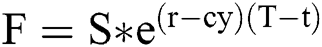 . Let the predicted value be
  , then the forecast value of the futures price of the three-factor model in the i-th period of the forecast period is:

The forecast value of the futures price of the six-factor model for the i-month period j in the forecast period is:

If the true value of the futures price is  , the index
  can be constructed to measure the degree of deviation of the predicted value from the true value, and
  is expressed as:

By comparing the  of the two models out of sample, the ability of the two models to predict the price of natural gas futures can be analyzed and evaluated.
4 Capability Assessment of Models in Natural Gas Pricing
The data used in this paper include the closing price of natural gas futures on the New York Mercantile Exchange (NYMEX) and the yield of US March Treasury bills. Due to the impact of the US shale gas revolution, the price of natural gas in the United States varies greatly after 2010. Therefore, the data in this paper will start from January 7, 2011 to April 26, 2019, the frequency of all data is week.
Due to the great time span of the sample, which exceeds the longest period of futures contracts traded on the exchange, we are unable to track the continuous price changes of all futures contracts during this period. Fortunately, since future contracts are standardized, we can ignore the contract itself, and focus only on the price change among contracts with same expiration date. Assume that the futures price due in recent month is  , the futures price due in the next consecutive month is
  , the futures price due in three consecutive months is
  , and so on. The data used in this paper include
  ,
,  ,
,  ,
,  ,
,  and
and  , where
  is equal to the spot price S.
Like any other commodity futures, natural gas futures do not have real spot prices and instantaneous convenience yields, so we use the price of futures contracts expire in recent months as spot prices. Based on futures due in recent month and near maturity, instantaneous convenience yield can be calculated using the method of Gibson et al. [1]: 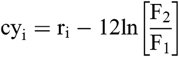 , in which
  is the annualized convenient yield rate at time i,
  is the annualized risk-free rate at time i,
  and
and  represent futures expired in two months and one month respectively. Due to the lack of spot prices, we use this approximation to calculate instantaneous convenience yields. Risk-free interest rates are measured using US March Treasury yields.
Fig. 1 shows the change in spot price S, logarithmic spot price X, instantaneous convenience yield cy, and risk-free interest rate r over time in seven years. It can be seen that before 2015, the convenience rate and risk-free rate both have a tendency towards to the long-term average, but in recent two years, they began to show an upward trend. Compare with them, there is no obvious trend in the development of spot prices during the sample period. It can be considered as random walk. Nielsen and Schwartz [41] pointed out that there is a negative correlation between inventory levels and convenience yields. The lower the inventory level, the greater the potential gains that spot holders may receive, and the higher the convenience yield. The development of sequences and convenience yield sequences is consistent with the conclusion of inventory theory.
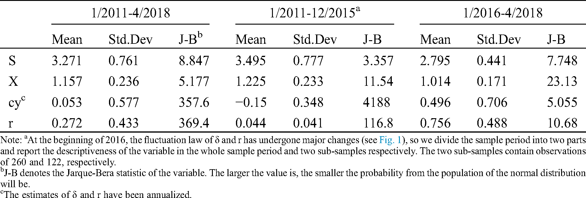
Thus, we divide the samples into two subsamples of varying lengths at the end of 2015, and report the main descriptive statistics for the above four variables in the total sample and the two subsamples in Tab. 1. It can be seen that for the two variables of convenience yield and risk-free interest rate, they obviously have larger mean and larger standard deviation in the second sub-sample period, and are also closer to the normal distribution. Difference between the mean and standard deviation of the spot price is not obvious in the two subsamples. Since the price S is converted to the logarithmic price X, the difference is further narrowed.
Since the convenience yield and risk-free interest rate cannot always follow the upward trend since 2016, from the whole sample period, we approximate that they generally obey the trend of returning to the long-term average. In summary, the development trend of the three factors of spot price, convenient yield and risk-free interest rate is in line with Schwartz’s [3] assumption that the three-factor model is used to price general commodity futures.

Figure 1: Evolution of S, X, cy and r
Table 1: Descriptive statistics
In order to verify the rationality of the six-factor model, it is necessary to demonstrate the seasonally adjusted sequence of factors. Before the seasonal adjustment, the weekly data need to be converted into monthly data. Our approach is to use the average of the weekly Data for each month as the data for that month. Fig. 2 shows the development of three factors in the sample period respectively.

Figure 2: Evolution of three factors. (a) Trend-cycle, (b) seasonal factors and (c) irregular component
It can be seen that the three sequences have significant periodic seasonal fluctuations. The cycle of the fluctuation is one year, and the value of the seasonal trend is almost equal in the same month in two consecutive years. Therefore, it is reasonable to use the seasonal trend value of each month in the last year of the sample as the seasonal trend value of the corresponding month outside the sample. In addition, the irregular changes of the three factors obviously trend to return to their long-term mean, but the mean of each factor is different. As for the general trend, it is basically the same shape as the original sequence, but with less subtle fluctuations. In general, we can assume that all the general trend factors and irregular change factors have a tendency to respond to the mean.
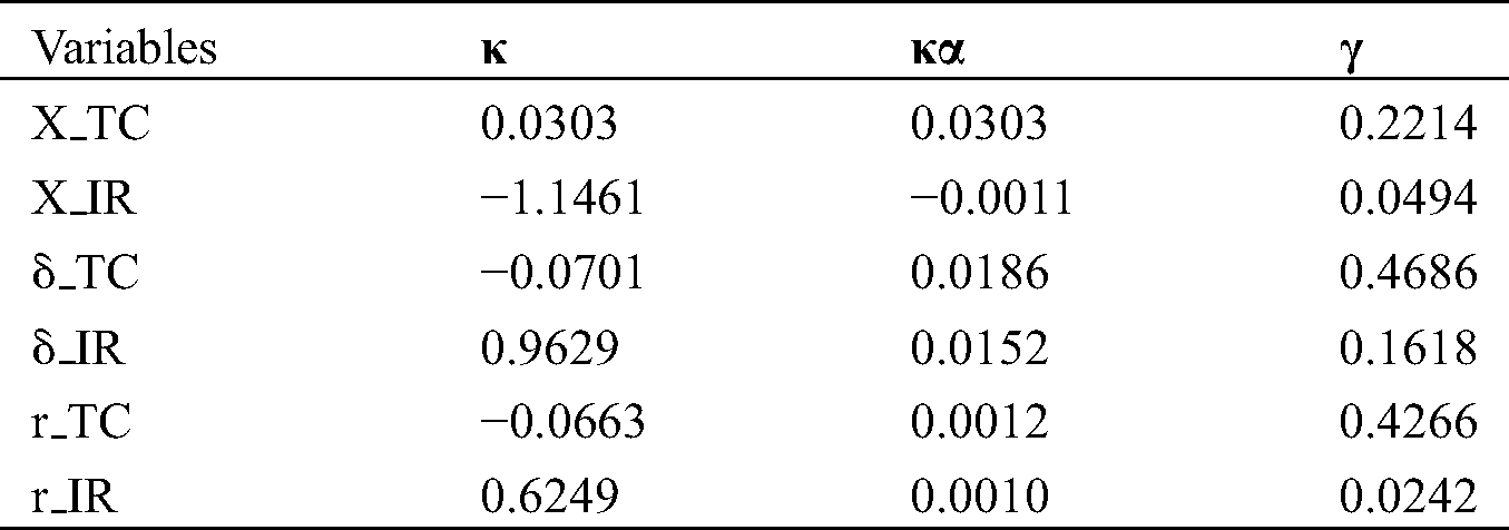
Using least squares regression and seemingly uncorrelated regression methods (Appendix A), the estimation results of all parameters in the three-factor model can be obtained according to Eqs. (6–8). We report these results in Tab. 2.
Table 2: Parameter estimation results of three-factor model
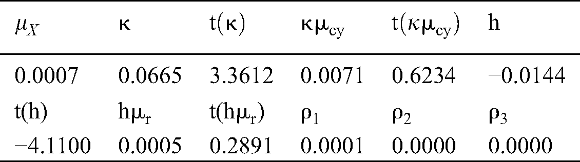
Obviously, although  is larger than
  and
and  , it is too small comparing with the estimated values in Schwartz [3]. In addition, during the total sample period, the estimates of κ and h are significantly different from zero, indicating that the convenience yield and the risk-free rate do have a tendency to respond to the mean, which supports our previous assumptions. The values of
  and h
and h are relatively small, and are not significantly different from 0, indicating that there are almost no fixed effects in the two discretization models (7) and (8).
Similarly, we report the parameter estimation results for the six-factor model in Tab. 3.
Table 3: Parameter estimation results of six-factor model
4.3 Comparison between Three-Factor Model and Six-Factor Model
With the results of the above parameter estimation, we then use the three-factor model and the six-factor model to predict the natural gas futures prices out of sample, and use the index  to evaluate the predictive power of the two models. The results of the assessment are shown in Tab. 4. And please see Appendix A for more detail.
Table 4: Fitting bias of three-factor model and six-factor model
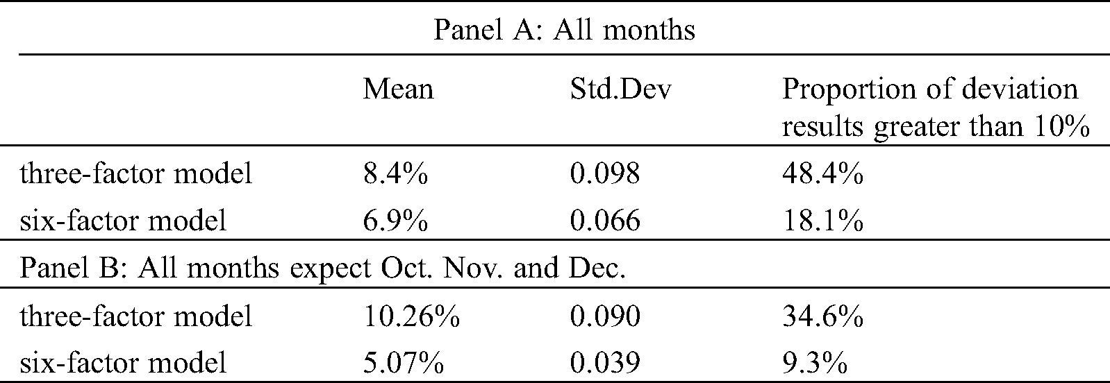
It can be seen that the relative deviations of the simulation results of the two models are 8.4% and 6.9%, respectively–the latter is smaller than the former, but the difference is small. Getting rid of Oct. Nov. and Dec., the values change to 10.26% and 5.07%, respectively–the former become larger, indicating that the fitting effect of the winter months is even better than the average monthly fit; The latter is further reduced to about 5%, indicating that after the three months of elimination, the overall effect of the fitting becomes better, and significantly better than the fitting effect of the three-factor model.
Comparing the standard deviations of two models, in general, the standard deviation of the prediction bias of the six-factor model is about 1/3 smaller than that of the three-factor model, and after elimination the winter months when the two models The poorly fitted, the gap has widened further and has become about 2/3. This shows that the six-factor model is more stable than the three-factor model.
It also can be seen that there is a large difference in the proportion of prediction errors between the two models. The greater than 10% proportion of the deviation between the predicted result of the three-factor model is 48.4%, and the value of six factor model is 18.1%. After excluding the winter months, the proportions are reduced to 34.6% and 9.3%, respectively. Obviously, the proportion of the larger prediction bias of the six-factor model is significantly smaller than that of the three-factor model, especially after the winter months are removed, making the possibility of the model causing extreme losses to investors becoming smaller.
Fig. 3a shows the tendency of the three-factor model’s prediction bias for  ,
,  , and
, and  in different months. It is found that for these three futures contracts, the forecast deviation is less different every month. Except for Oct. Nov. and Dec., the forecast deviation is basically less than 10%. Fig. 3b shows the development of the prediction bias of the six-factor model for
  ,
,  , and
, and  in different months. Compared with Fig. 3a, the trend of the curve is basically the same, and in the winter months, the prediction bias of the model is still very large, indicating that we have not significantly improved the seasonal adjustment of the model in the winter months.

Figure 3: Fitting results for  ,
, ,
,  . (a) Three-factor model and (b) six-factor model
Fig. 4 shows the fitting effects of the three-factor model and the six-factor model on  ,
,  , and
, and  . It shows that when the term of the futures contract becomes longer, the predicted deviation of the model has no obvious trend, but becomes a fluctuation within a certain range. The difference is that the range of relative deviation fluctuations of the six-factor model is smaller than the three-factor model in each period, especially
  and
and  —the former are below 8%, and the latter are all within 12%. It shows that for longer-term contracts, the predictive power of the six-factor model is greatly improved compared with the three-factor model.

Figure 4: Fitting results for  ,
, ,
,  . (a) Three-factor model and (b) six-factor model
In summary, after seasonal adjustment of the three-factor model, the model’s ability to predict natural gas futures prices has been significantly improved, and it has become more stable. Therefore, for natural gas futures, the six-factor model perform better than the three-factor model.
5 Natural Gas Futures Price Forecast
According to the above analysis, the relative deviation of natural gas futures price can be controlled in a lower level of about 5% (except in winter) by adopting six-factor model. In this section, we will use the six-factor model to predict the price of natural gas futures contracts from May 2019 to April 2020 (Based on historical data, prices can be predicted in any period. We need to reestimate the parameters in the model based on the latest historical data in that case.).
We first add the off-sample data to the sample and updated the model’s parameters and the initial values used for the prediction. We report the updated parameter estimates in Tab. 5, and report the projected prices for monthly natural gas futures contracts in Tab. 6.
Table 5: Updated parameter estimation results
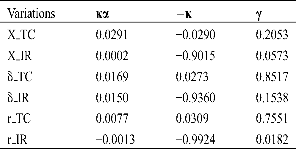
Table 6: The predicted price of  -
- per month for the coming year

Tab. 6 shows the forecast values. It is should be noticed that the test results out of sample show that although the changed model improves the forecasting ability in the winter months, the predicted deviation is still large, and the actual price in winter is always higher than the price predicted by the model. Therefore, the forecast results for the three months of October, November and December in Tab. 6 should be lower than the actual values.
Fig. 5 shows the trend of prices for each term contract in different months. It can be seen that before October, the price of the contract has a rise trend to rise over time, and after reaching the highest value in October and November, there is a downward trend. In February of the second year, there was an upward trend. Considering the performance of the model outside the sample, in the winter months, the results of the fitting tend to be smaller than the actual value. Therefore, the actual price fluctuation of  should be more strong than the curve in Fig. 5.
The futures prices of each term have a strong rise trend. Compared with them, the trend of spot prices is less obvious, but our price prediction for each month can provide investors with a reference. Even this reference might be more useful.

Figure 5: Prices of  -
-  in different months

Figure 6: Monthly contract price for different terms
Fig. 6 shows the trend of contract prices as the contract period increases each month. In general, the trend of contract price increase with the term is consistent in each month, that is, the contract price decreases with the increase of the term before 3 months, from the  to the
  price. After reaching the highest value, it began to drop sharply and began to rise slightly to
  .
.
6 Conclusions and Policy Recommendations
In the next 20 years, natural gas will become more and more important in the use of energy because it is the most important energy source for the transition of fossil energy to clean energy. Studying the pricing rules of natural gas market and natural gas futures is the focus of this paper.
Natural gas future is a special commodity futures. The pricing law of natural gas is different from that of general commodity futures due to its obvious characteristic of seasonal variation. Thus, the classic three-factor model will leads to significant deviation when used for natural gas futures pricing.
Given the characteristic of natural gas futures, we developed a six-factor model with seasonal adjustment based on the three-factor model. Each factor in three-factor model of Schwartz [1] is decomposed into three sub-factors: general trend factor, seasonal trend factor and irregular change factor. Monte Carlo simulation method is introduced to compare the predictive performance of the six-factor model with the three-factor model. The results show that: (1) The prediction bias of the six-factor model is smaller than that of three-factor model remarkably with an average deviation of only 6.9% out of sample. (2) By comparison, we find the maximum prediction deviation of the six-factor model is 27.2% which is much smaller than that of the three-factor model. (3) For the prediction of natural gas prices in winter months, the average prediction bias of the six-factor model is 12.5%, compared with the three-factor model, the reduction is 6.2%. (4) The six-factor model is more suitable for natural gas futures pricing, indicating that it is necessary to consider seasonal fluctuations in the model. Further, after updating the parameters, we use the six-factor model to predict the spot price and the contract price of each term in each month from May 2019 to April 2020. The forecast results show that the prices of all futures contracts increase over time, with spot prices reaching their maximum in November and their minimum in February. In any month, the contract price of 8 months is the highest, and the contract price of 10 months is the lowest.
The research results provide a new way to improve the accuracy of natural gas futures price predictions, which will help natural gas market stakeholders to more accurately grasp the future price trend of the natural gas market and provide reference for decision makers and investors. It is worth noting that the basis of this model is the law of movement of historical data. We suggest that when predicting the price of natural gas futures in the future, the parameters in the model should be re-estimated based on the latest data. The estimate method proposed by this paper can also be used under that circumstance.
Acknowledgement: This work was supported by the National Natural Science Foundation of China (Nos. 71704080, 71774087, 71403131), the Fundamental Research Funds for the Central Universities (No. 30917013101), the Research Foundation of School of Economics and Management of Nanjing University of Science and Technology for the Young Scholar (JGQN1704), the Cultural Experts and “Four batch” Talents Independently Selected Topic Project (ZXGZ[2018]86), and the Jiangsu Province Natural Science Foundation of China (BK20171422), and Jiangsu Province Graduate Research and Practice Innovation Plan (KYCX19_0210).
Funding Statement: The authors received no specific funding for this study.
Conflicts of Interest: The authors declare that they have no conflicts of interest to report regarding the present study.
1. Brennan, M. J. (1979). The pricing of contingent claims in discrete time models. The Journal of Finance, 34. DOI 10.1111/j.1540-6261.1979.tb02070.x. [Google Scholar] [CrossRef]
2. Gibson, R., Schwartz, E. S. (1990). Stochastic convenience yield and the pricing of oil contingent claims. Journal of Finance, 45(3), 959–976. DOI 10.1111/j.1540-6261.1990.tb05114.x. [Google Scholar] [CrossRef]
3. Schwartz, E. S. (1997). The stochastic behavior of commodity prices: Implications for valuation and hedging. Journal of Finance, 52(3), 923–973. DOI 10.1111/j.1540-6261.1997.tb02721.x. [Google Scholar] [CrossRef]
4. Miltersen, K. R., Schwartz, E. S. (1998). Pricing of options on commodity futures with stochastic term structures of convenience yields and interest rates. Journal of Financial and Quantitative Analysis, 33(1), 33–59. DOI 10.2307/2331377. [Google Scholar] [CrossRef]
5. Casassus, J., Collin-Dufresne, P. (2005). Stochastic convenience yield implied from commodity futures and interest rates. Journal of Finance, 60(5), 2283–2331. DOI 10.1111/j.1540-6261.2005.00799.x. [Google Scholar] [CrossRef]
6. Liu, P., Tang, K. (2011). The stochastic behavior of commodity prices with heteroskedasticity in the convenience yield. Journal of Empirical Finance, 18(2), 211–224. DOI 10.1016/j.jempfin.2010.12.003. [Google Scholar] [CrossRef]
7. Chen, Z., Forsyth, P. A. (2010). Implications of a regime-switching model on natural gas storage valuation and optimal operation. Quantitative Finance, 10(2), 159–176. DOI 10.1080/14697680802374791. [Google Scholar] [CrossRef]
8. Chen, S. (2010). Modelling the dynamics of commodity prices for investment decisions under uncertainty. UWSpace Home, University of Waterloo. http://hdl.handle.net/10012/5504. [Google Scholar]
9. Lammerding, M., Stephan, P., Trede, M. (2013). Speculative bubbles in recent oil price dynamics: Evidence from a Bayesian Markov-switching state-space approach. Energy Economics, 36, 491–502. DOI 10.1016/j.eneco.2012.10.006. [Google Scholar] [CrossRef]
10. Almansour, A. (2016). Convenience yield in commodity price modeling: A regime switching approach. Energy Economics, 53, 238–247. DOI 10.1016/j.eneco.2014.06.016. [Google Scholar] [CrossRef]
11. Cortazar, G., Lopez, M., Naranjo, L. (2017). A multifactor stochastic volatility model of commodity prices. Energy Economics, 67, 182–201. DOI 10.1016/j.eneco.2017.08.007. [Google Scholar] [CrossRef]
12. Baur, D. G., Dimpfl, T. (2018). The asymmetric return-volatility relationship of commodity prices. Energy Economics, 76, 378–387. DOI 10.1016/j.eneco.2018.10.022.
13. Bohl, M. T., Sulewski, C. (2019). The impact of long-short speculators on the volatility of agricultural commodity futures prices. Journal of Commodity Markets, 16, 100085. DOI 10.1016/j.jcomm.2019.01.001.
14. Knaut, A., Paschmann, M. (2019). Price volatility in commodity markets with restricted participation. Energy Economics, 81, 37–51. DOI 10.1016/j.eneco.2019.03.004.
15. Hahn, W. J., DiLellio, J. A., Dyer, J. S. (2018). Risk premia in commodity price forecasts and their impact on valuation. Energy Economics, 72, 393–403. DOI 10.1016/j.eneco.2018.04.018.
16. He, C., Jiang, C., Molyboga, M. (2019). Risk premia in Chinese commodity markets. Journal of Commodity Markets, 15, 100075.1–100075.18. DOI 10.1016/j.jcomm.2018.09.003.
17. Li, B. (2018). Speculation, risk aversion, and risk premiums in the crude oil market. Journal of Banking & Finance, 95, 64–81. DOI 10.1016/j.jbankfin.2018.06.002.
18. Andreasson, P., Bekiros, S., Nguyen, D. K. (2016). Impact of speculation and economic uncertainty on commodity markets. International Review of Financial Analysis, 43, 115–127. DOI 10.1016/j.irfa.2015.11.005.
19. Bakas, D., Triantafyllou, A. (2018). The impact of uncertainty shocks on the volatility of commodity prices. Journal of International Money and Finance, 87, 96–111. DOI 10.1016/j.jimonfin.2018.06.001.
20. Bakas, D., Triantafyllou, A. (2019). Volatility forecasting in commodity markets using macro uncertainty. Energy Economics, 81, 79–94. DOI 10.1016/j.eneco.2019.03.016.
21. Gómez-Valle, L., Habibilashkary, Z., Martínez-Rodríguez, J. (2017). A new technique to estimate the risk-neutral processes in jump–diffusion commodity futures models. Journal of Computational and Applied Mathematics, 309, 435–441. DOI 10.1016/j.cam.2015.12.028.
22. Dempster, M. A. H., Medova, E., Tang, K. (2018). Latent jump diffusion factor estimation for commodity futures. Journal of Commodity Markets, 9, 35–54. DOI 10.1016/j.jcomm.2018.01.001.
23. Da Fonseca, J., Ignatieva, K. (2019). Jump activity analysis for affine jump-diffusion models: Evidence from the commodity market. Journal of Banking & Finance, 99, 45–62. DOI 10.1016/j.jbankfin.2018.11.014.
24. Nguyen, D. B. B., Prokopczuk, M. (2019). Jumps in commodity markets. Journal of Commodity Markets, 13, 55–70. DOI 10.1016/j.jcomm.2018.10.002. [Google Scholar] [CrossRef]
25. Zhang, D., Shi, M., Shi, X. (2018). Oil indexation, market fundamentals, and natural gas prices: An investigation of the Asian premium in natural gas trade. Energy Economics, 69, 33–41. DOI 10.1016/j.eneco.2017.11.001. [Google Scholar] [CrossRef]
26. Brown, S. P., Yücel, M. K. (2008). What drives natural gas prices? Energy Journal, 29(2), 45–60. DOI 10.5547/ISSN0195-6574-EJ-Vol29-No2-3. [Google Scholar] [CrossRef]
27. Hartley, P. R., Medlock, I. I. I. K. B. (2014). The relationship between crude oil and natural gas prices: The role of the exchange rate. Energy Journal, 35(2), 25–44. DOI 10.5547/01956574.35.2.2.
28. Batten, J. A., Ciner, C., Lucey, B. M. (2017). The dynamic linkages between crude oil and natural gas markets. Energy Economics, 62, 155–170. DOI 10.1016/j.eneco.2016.10.019.
29. Ji, Q., Zhang, H. Y., Geng, J. B. (2018). What drives natural gas prices in the United States?–A directed acyclic graph approach. Energy Economics, 69, 79–88. DOI 10.1016/j.eneco.2017.11.002. [Google Scholar] [CrossRef]
30. Brigida, M. (2014). The switching relationship between natural gas and crude oil prices. Energy Economics, 43, 48–55. DOI 10.1016/j.eneco.2014.01.014. [Google Scholar] [CrossRef]
31. Renou-Maissant, P. (2012). Toward the integration of European natural gas markets: A time-varying approach. Energy Policy, 51, 779–790. DOI 10.1016/j.enpol.2012.09.027. [Google Scholar] [CrossRef]
32. Wiggins, S., Etienne, X. L. (2017). Turbulent times: Uncovering the origins of US natural gas price fluctuations since deregulation. Energy Economics, 64, 196–205. DOI 10.1016/j.eneco.2017.03.015. [Google Scholar] [CrossRef]
33. Lucía, J., Schwartz, E. S. (2002). Electricity prices and power derivatives: Evidence from the Nordic power exchange. Review of Derivatives Research, 5(1), 5–50. DOI 10.1023/A:1013846631785. [Google Scholar] [CrossRef]
34. Cartea, A., Figueroa, M. G. (2005). Pricing in electricity markets: A mean reverting jump diffusion model with seasonality. Applied Mathematical Finance, 12(4), 313–335. DOI 10.1080/13504860500117503. [Google Scholar] [CrossRef]
35. Amin, K., Ng, V., Pirrong, S. C. (1995). Valuing energy derivatives, chapter 3 in managing energy price risk. pp. 57–70, Risk Publications. [Google Scholar]
36. Borovkova, S., Geman, H. (2006). Seasonal and stochastic effects in commodity forward curves. Review of Derivatives Research, 9(2), 167–186. DOI 10.1007/s11147-007-9008-4. [Google Scholar] [CrossRef]
37. Mirantes, A. G., Población, J., Serna, G. (2013). The stochastic seasonal behavior of energy commodity convenience yields. Energy Economics, 40, 155–166. DOI 10.1016/j.eneco.2013.06.011. [Google Scholar] [CrossRef]
38. Mirantes, A. G., Población, J., Serna, G. (2012). The stochastic seasonal behavior of natural gas prices. European Financial Management, 18(3), 410–443. DOI 10.1111/j.1468-036X.2009.00533.x. [Google Scholar] [CrossRef]
39. Mankiw, N. G., Miron, J. A. (1991). Should the Fed smooth interest rates? The case of seasonal monetary policy//Carnegie-Rochester Conference Series on Public Policy, North-Holland, 34, 41–69. [Google Scholar]
40. Mikutowski, M., Karathanasopoulos, A., Zaremba, A. (2019). Return seasonalities in government bonds and macroeconomic risk. Economics Letters, 176, 114–116. DOI 10.1016/j.econlet.2019.01.012. [Google Scholar] [CrossRef]
41. Nielsen, M. J., Schwartz, E. S. (2004). Theory of storage and the pricing of commodity claims. Review of Derivatives Research, 7(1), 5–24. DOI 10.1023/B:REDR.0000017026.28316.c8. [Google Scholar] [CrossRef]
Appendix A. Least squares regression and seemingly uncorrelated regression methods


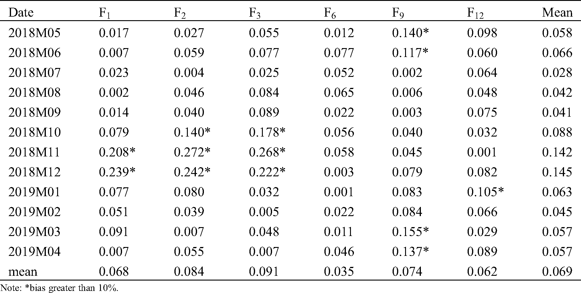
Appendix B. Predictive deviation matrix for three-factor model and six-factor model
Table A: Bias of three-factor model
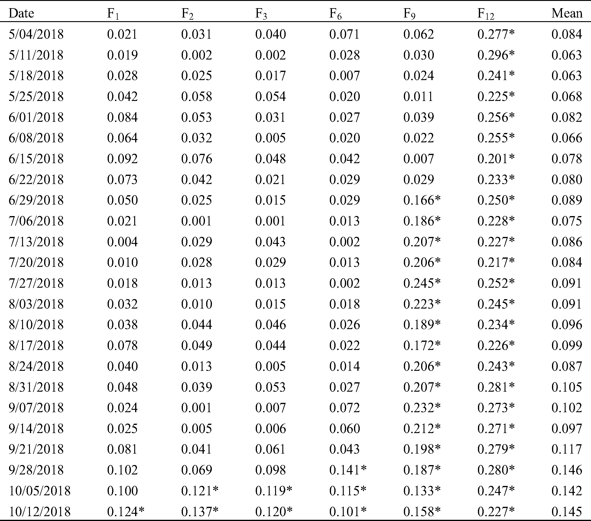
Note: *bias greater than 10%.
Table B: Bias of six-factor model
 | This work is licensed under a Creative Commons Attribution 4.0 International License, which permits unrestricted use, distribution, and reproduction in any medium, provided the original work is properly cited. |