Energy Engineering

DOI: 10.32604/EE.2021.014868

ARTICLE

A Novel Power Curve Prediction Method for Horizontal-Axis Wind Turbines Using Artificial Neural Networks

Vin Cent Tai1,*, Yong Chai Tan1, Nor Faiza Abd Rahman1, Chee Ming Chia2, Mirzhakyp Zhakiya2 and Lip Huat Saw3

1Centre for Modelling and Simulation, Faculty of Engineering, Built Environment and Information Technology, SEGi University, Petaling Jaya, 47810, Malaysia
2Mechanical Engineering Department, Faculty of Engineering, Built Environment and Information Technology, SEGi University, Petaling Jaya, 47810, Malaysia
3Lee Kong Chian Faculty of Engineering and Science, UTAR, Kajang, 43200, Malaysia
*Corresponding Author: Vin Cent Tai. Email: taivincent@segi.edu.my
Received: 04 October 2020; Accepted: 13 January 2021

1  Introduction

Modelling of wind turbines is important in windfarm planning for accurate prediction of power production [1]. In early stage of the windfarm development low fidelity models such as empirical and regression models are used to predict the wind energy production, due to many variables such as the turbine diameter, hub-height, power curve characteristics, etc., are yet to be determined in the early stage of planning. Therefore, it is important to develop a low fidelity model with reasonable accuracy for use in early stage of windfarm planning to improve the robustness, such way to reduce the design looping and time required in the development stage. While there exists a lot of methods for wind turbine power curve modelling in the literatures [2–4], such methods are only suitable for modelling one specific type of wind turbine at a time to predict the power output at given wind speeds.

Fig. 1 depicts the power curve of a typical pitch-controlled Horizontal-Axis Wind Turbine (HAWT). The wind velocity which the wind turbine started to produce energy is cut-in speed, uc . As wind speed increases, the energy production increases until the rated power, Pr is reached. The wind speed that corresponds to the rated power is known as rated speed, ur . For pitch controlled HAWT, the rotor blade angle is controlled to keep the power output at Pr for wind speed above ur . When the wind speed exceeded the cut-out speed ( uo ), the wind turbine is shut down to avoid damage. On the other hand, active stall-controlled HAWT resembles pitch-controlled HAWT as both HAWTs are equipped with pitch-able blades to produce constant power at high wind speeds. The difference between pitch-controlled and active stall-controlled mechanisms occurs in the operation of HAWT at high wind speeds. While pitch-control mechanism decreases the angle-of-attack of the blades to reduce the lift force at high wind speeds, active stall-control mechanisms increases the angle-of-attack to stall the blades [5].

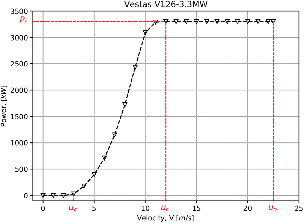
Figure 1: Typical characteristics of a pitch/active stall controlled HAWT power curve

Conventional methods based on Blade Element Momentum (BEM) theory [6,7] require detailed geometry of the HAWT for performance prediction. Such physics-based methods involve dividing up the blade into a finite number of elements and calculating the flow at each one and subsequently performing numerical integration along the blade span to obtain the performance characteristics. Brake State Models (BSM) are often used together with BEM to obtain the axial and tangential induction factors (denoted by a and a′ , respectively) [8–12]. Given the detailed geometrical and aerodynamic information of a wind turbine, BEM can produce reasonably accurate performance prediction with about 20% uncertainty in blade load estimation [13]. However, such information may not be available in the early stage of wind farm planning as the geometry data are often kept confidential by turbine manufacturers.

In recent years, parametric and non-parametric regression methods have received a lot of attention for wind turbine power curve modelling for on-site condition monitoring of wind turbines. Parametric models such as polynomials [14–16] and logistic equations [17,18] have been used to fit the nonlinear region of the power curve (see Fig. 1) based on manufacturers or on-site wind power output data. Non-parametric methods such as Artificial Neural Network (ANN) [19,20], fuzzy logic [21], and data mining [22] methods have also been widely investigated. However, such methods are site-specific and do not express the relationship between the turbine design information and its power outputs.

To the authors’ knowledge, there is no method that would produce a power curve for a given set of basic wind turbine design information such as turbine diameter, rated speed, etc. In view of this, this work is dedicated to close the loop by formulating a modelling architecture that relates the design information and its power production using ANN. The remaining of the paper is organized as follows: a brief review of ANN and assumptions used in developing the model are described in Section 2, followed by results and discussion in Section 3, and conclusions are presented in Section 4.

2  Power Curve Modelling Architecture

Fig. 2 depicts the Multi-Layer Perceptron (MLP) ANN architecture for this study. ANN is a mathematical model that mimics the function of biological neural systems [20,23]. It consists of an input layer of six input units, three hidden layers with five neuron units each, and an output layer of twenty-six output units for power curve profile (i.e., normalised power curve) from velocity 0 to 25 m/s with 1 m/s interval. All the units (i.e., neurons) are fully connected in a feed-forward fashion. A total of fifteen hidden neurons were chosen in this study following the general rule-of-thumb that the number of hidden neurons should be in between twice the number of input layer and 2/3 of input plus output layers [24,25]. Three hidden layers was chosen to evenly distribute the total number of hidden neurons.

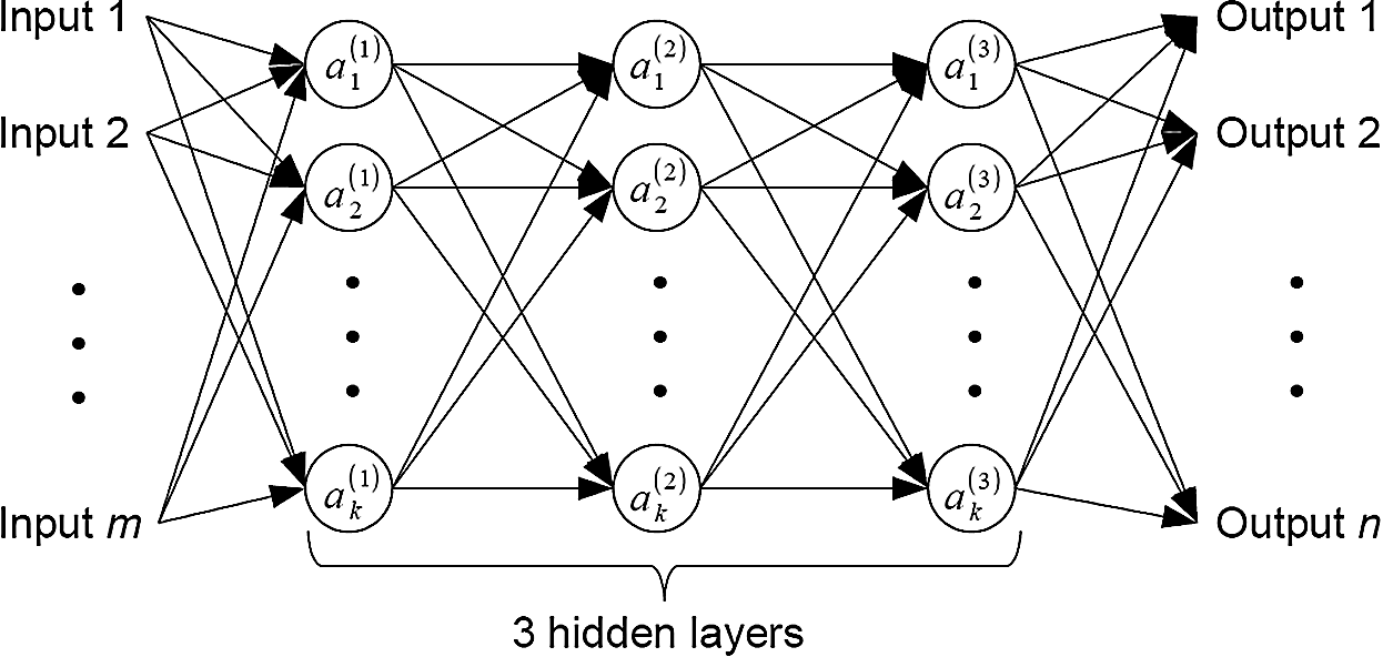
Figure 2: The MLP ANN architecture used for present study

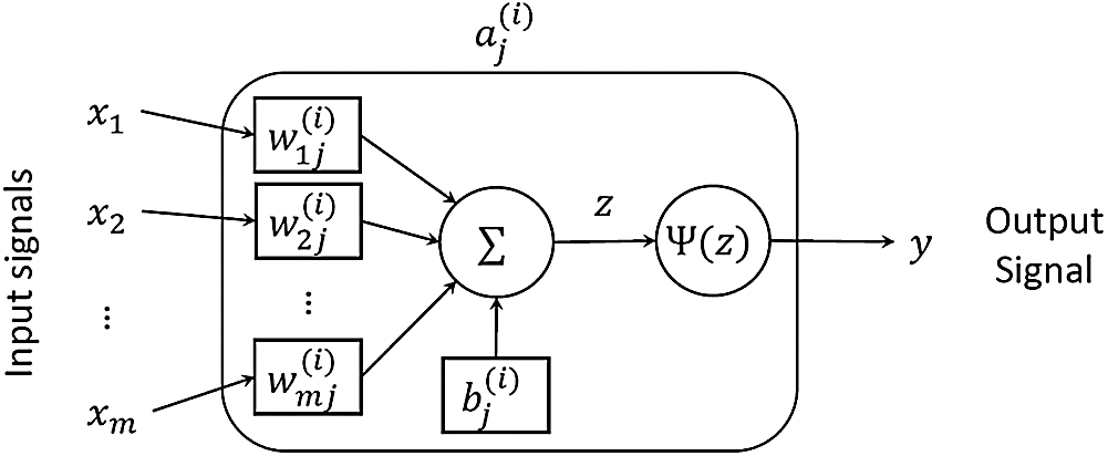
Figure 3: Illustration of perceptron model of neuron aj(i)

Each neuron is modelled as depicted in Fig. 3 known as perceptron. Mathematically, the process of jth neuron in layer ith releases signal y when reacts to input signal {x1,x2,⋅⋅⋅,xm} is as follows:

z=∑km⁡wkj(i)xk+bj(i) (1)

y=Ψ(z)=max(0,z) (2)

where, wkj(i) is the weight assigned to the kth input signal, b is a constant known as bias, and Ψ(⋅) is activation function. In the present study, Rectified Linear Unit (ReLU) activation function has been employed due to its ability to solve vanishing gradient problems and faster in computation [26,27]. Learning of input-output signals was realised using Back-propagation algorithm. Adaptive Moments (Adam) optimisation [28] has been used to minimise the objective function, ℓ (i.e., the objective function) by iteratively adjusting the weights during the learning phase:

ℓ=1n∑i=1n⁡(Yi−Y^i)2+λ∑j=1m⁡wj2 (3)

The first term of the objective function is Mean Squared Error (MSE) of the model and targeted outputs for all n number of outputs. The second term of the loss equation is penalty function known as L2-regularization, which consists of a regularisation constant λ for all m number of weights. In conjunction with Back-propagation algorithm, L2-regularization helps to improve the model generalisation by penalising large weight values during the learning phase. In this study, λ=0.001 has been used. On top of that, early stopping is activated when ℓ stopped to improve for 100 successive epochs, such way to prevent overfitting and improve model generalisation.

A total of one hundred and ninety-eight existing pitch-controlled and active stall-controlled wind turbines consisted of two and three blades have been considered in this study. The wind turbines are split into 7:3 ratio by random for ANN training and testing, respectively. All wind speeds of the wind turbine power curves ( udat ) at their published air density ( ρdat ) obtained from [29–31] were corrected to wind speeds ( ustd ) at standard air density of ρstd=1.225 kg/m3 using Eq. (4). Then, the power curves with corrected wind speeds ( Pcor ) were normalised against their respective ur using Eq. (5) to yield the power curve profiles ( p ) for ANN training.

ustd=udat(ρdatρstd)13 (4)

p=PcorPr (5)

To further improve the model generalization of ANN, a total of ten independent ANN models have been created, as depicted in Fig. 4. The final output of predicted power curve is the averaged output of all the ten independent ANN models. Based on the features of a typical pitch controlled and active stall controlled HAWT power curve, a total of six parameters, i.e., Pr , ur , uc , uo , rotor diameter ( D ), and number of blades ( nb ) have been selected as model inputs. The modelling is realised with TensorFlow, a Google’s open-source modelling framework for ANN and deep learning [32,33].

Figure 4: The overview of ensemble ANN model for the present study

3  Results and Discussion

Fig. 5 shows the cross-validation plot of calculated power versus actual power for all the 198 HAWTs. A total of 18 power curves have been sampled for comparison purposes, with 6 best fitted power curves as presented in Fig. 6, 6 averagely fitted curves in Figs. 7 and 6 worst fitted results in Fig. 8. The figures show that the proposed method is reliable and reasonably accurate to capture the power curve trends.

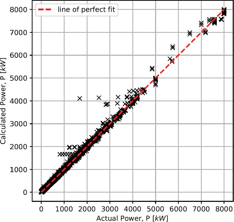
Figure 5: Cross-validation plot of calculated and actual data for a total of 198 wind turbines

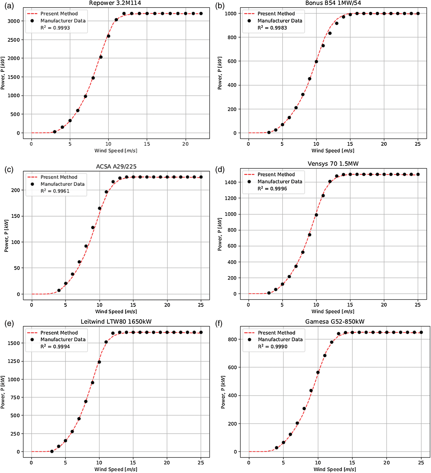
Figure 6: Sample of best-fit power curves

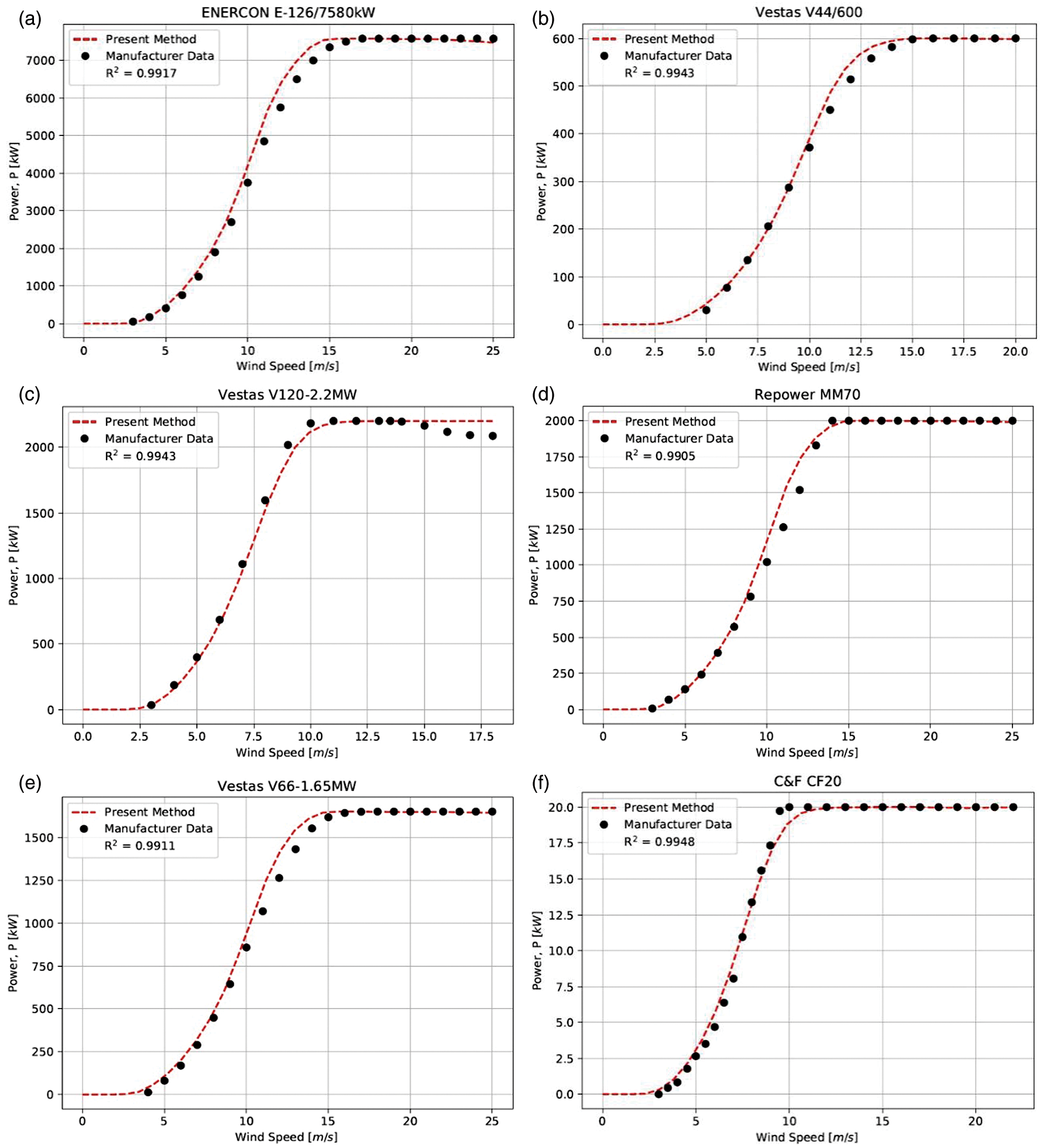
Figure 7: Sample of average-fit power curves

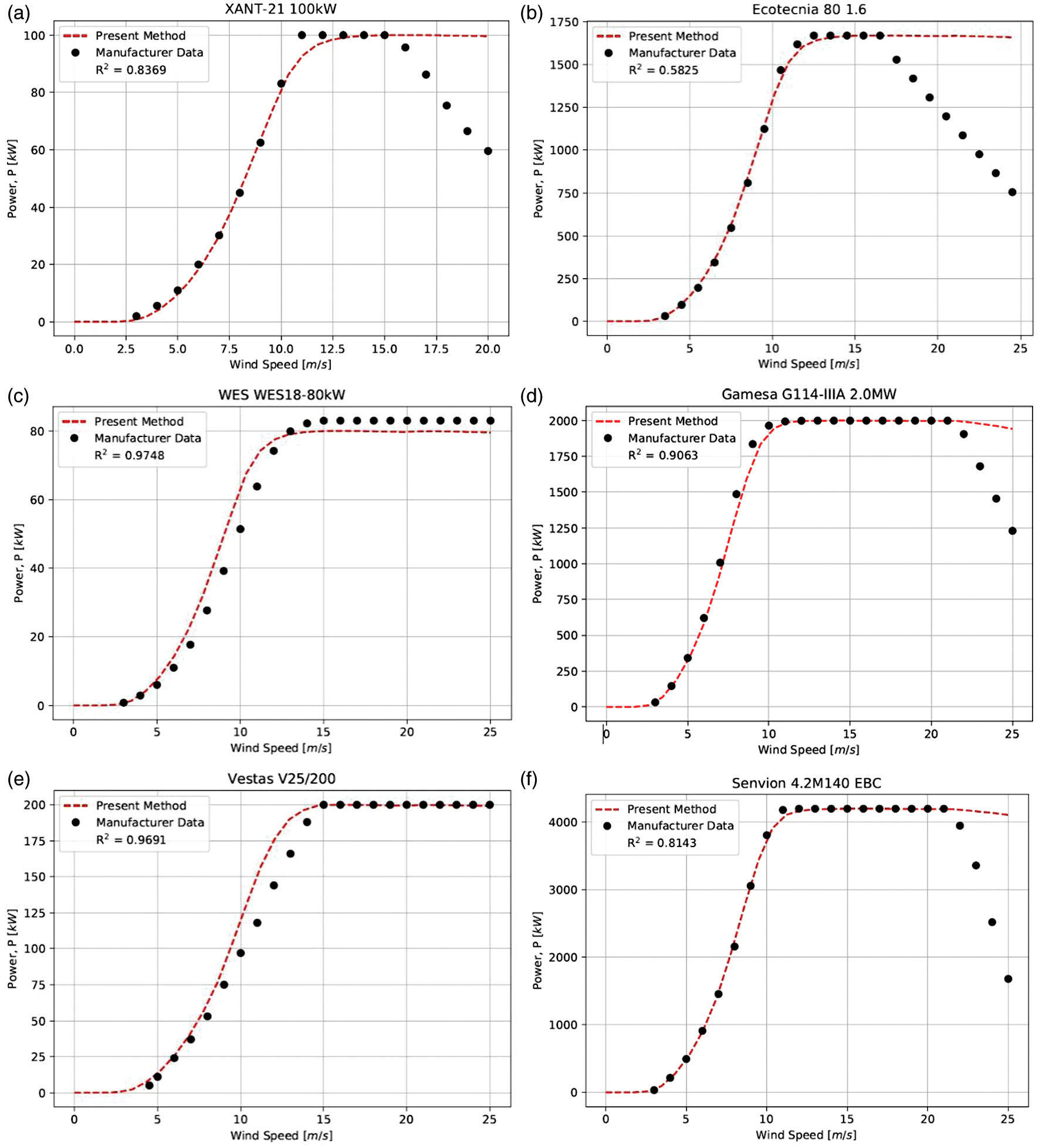
Figure 8: Sample of worst-fit power curves

R2 was used to quantify the performance of the proposed method. The R2 value for the cross-validation plot (Fig. 5) is 0.9966, indicating the proposed method is reasonably accurate in general. Out of the 198 wind turbines, the maximum R2 is 0.9996 for Vensys 70 1.5 MW wind turbine (see Fig. 6d) and the minimum value is 0.5825 for Ecotecnia 80 1.6 wind turbine (see Fig. 8b). The average value of R2 shows that the proposed method is accurate. The proposed method tends to predict constant power in the speed range of ur<V≤uo , which is typical for most pitch controlled HAWT.

However, a close examination on Figs. 8a, 8b, 8d and 8f revealed that the proposed method performs poorly for HAWTs that possess soft cut-out control strategy which gradually ramping down energy production at high wind speeds to avoid overloading on turbine blades [34]. This attributes to only a few HAWTs with such derating feature were included in the ANN training, therefore lack of information available for the proposed method to learn the underlying relationships between the input and output variables. For the speed range between uc and um , the proposed method can capture the trends reasonably well.

4  Conclusions

In this work, a simple MLP ANN method for power curve estimation has been proposed. The proposed method receives 6 basic wind turbine design information ( Pr , uc , ur , uo , D , and nb ) to predict its power curve from 0 m/s to maximum 25 m/s. Although it is not a perfect fit to the actual power curve data, validation of the method against all 198 existing wind turbines from 5 kW to 8 MW showed that the method is reasonably accurate and reliable in general, with average R2 score of 0.9966. However, the proposed method performs poorly for HAWTs equipped with soft cut-out control strategy that gradually ramping down energy production before uo , due to lack of HAWTs with such feature had been used in ANN training.

In conventional wind turbine design, detailed geometry of the wind turbine has to be generated before its aerodynamic properties and power curve can be evaluated using physics-based methods such as BEM or high-fidelity numerical simulations such as Computational Fluid Dynamics. In the present study, historical data of wind turbines have been used to generate a low fidelity model using ANN. Unlike the existing parametric and non-parametric power curve modelling methods for on-site condition monitoring of wind turbines, the method proposed in this study is the best-known method to estimate the power curve without having to account for detailed wind turbine geometry and its aerodynamic properties, hence it provides a quick means for applications such as wind turbine design optimisation as well as windfarm planning and windfarm optimisation.

Funding Statement: The project is funded by the Ministry of Higher Education Malaysia, under the Fundamental Research Grant Scheme (FRGS Grant No. FRGS/1/2016/TK07/SEGI/02/1).

Conflicts of Interest: The authors declare that they have no conflicts of interest to report regarding the present study.

This work is licensed under a Creative Commons Attribution 4.0 International License, which permits unrestricted use, distribution, and reproduction in any medium, provided the original work is properly cited.