| Energy Engineering |
DOI: 10.32604/EE.2021.014515
ARTICLE
Research on Direct Yaw Moment Control Strategy of Distributed-Drive Electric Vehicle Based on Joint Observer
1CCCC Second Highway Consultants Co., Ltd., Wuhan, 430056, China
2School of Automobile, Chang’an University, Xi’an, 710064, China
3Shaanxi Fast Auto Drive Group Co., Ltd., Xi’an, 710119, China
*Corresponding Author: Zichen Zheng. Email: zhengzichen@chd.edu.cn
Received: 04 October 2020; Accepted: 12 November 2020
Abstract: Combined with the characteristics of the distributed-drive electric vehicle and direct yaw moment control, a double-layer structure direct yaw moment controller is designed. The upper additional yaw moment controller is constructed based on model predictive control. Aiming at minimizing the utilization rate of tire adhesion and constrained by the working characteristics of motor system and brake system, a quadratic programming active set was designed to optimize the distribution of additional yaw moments. The road surface adhesion coefficient has a great impact on the reliability of direct yaw moment control, for which joint observer of vehicle state parameters and road surface parameters is designed by using unscented Kalman filter algorithm, which correlates vehicle state observer and road surface parameter observer to form closed-loop feedback correction. The results show that compared to the “feedforward + feedback” control, the vehicle’s error of yaw rate and sideslip angle by the model predictive control is smaller, which can improve the vehicle stability effectively. In addition, according to the results of the docking road simulation test, the joint observer of vehicle state and road surface parameters can improve the adaptability of the vehicle stability controller to the road conditions with variable adhesion coefficients.
Keywords: Vehicle stability control; distributed drive; direct yaw moment control; joint observer
When the vehicle is sharp turning at high speed, the limited tire adhesion force cannot provide enough lateral force, which will lead to the tire lateral force exceeding the adhesion limit and cause rollover and sideslip. For vehicle instability in extreme conditions, the researchers put forward the direct yaw moment control strategy. The control strategy adjusts the driving and brake torque of each wheel on basis of the current vehicle state for producing the yaw moment to improve the vehicle stability. So the yaw rate and sideslip angle of the vehicle can be controlled within the scope of the stability to maintain the vehicle stability. Distributed-drive electric vehicle which has the flexible driving form creates the ideal conditions for vehicle stability control. But compared with the traditional fuel vehicles, the complexity in the dynamic characteristics, actuator response characteristics and the actuator of distributed-drive electric vehicles are increased. For the stability control system of distributed-drive electric vehicle, we need to conduct specialized research.
According to the structure of the control system, the vehicle stability control system can be divided into the centralized vehicle stability controller and the hierarchical vehicle stability controller. The hierarchical controller can realize the decoupling between different systems, improve the transient control performance of each systems and reduce the controller complexity [1]. The commonly used algorithms include proportional integral and differential control (PID), fuzzy logic control, robust control, sliding mode control, model predictive control and so on.
Wang et al. [2] proposed a stability control method based on integral separation PID. At the beginning and end of the control, the PID controller does not consider the integral term, so as to eliminate integral accumulation error of control system. The controller can also determine the parameters of the PID controller based on the road adhesion coefficient by using logical threshold control. Zhai et al. [3] proposed a vehicle stability control method based on fuzzy PID. According to the phase plane method to determine the stable state of the vehicle, the upper level controller included a speed tracking controller, a yaw moment controller, and four wheel-slip controllers. The speed tracking controller adopted PID algorithm to calculate the desired value of traction force to follow the expected speed. The yaw moment controller used the fuzzy PID algorithm to calculate the additional yaw moment. However, the use of PID algorithm cannot guarantee the optimal or stability control for system [4].
Boada et al. [5] proposed a vehicle stability control method based on fuzzy logic control, and adopted the average maximum membership method to solve the fuzzy and determine the additional yaw moment. Zhao et al. [6] and Xiao et al. [7] proposed a vehicle stability control method based on T-S fuzzy theory. The nonlinear three-degrees-of-freedom vehicle dynamics model is transformed into a T-S fuzzy model with four linear subsystems, and a feedback controller of Parallel Distributed Compensation (PDC) framework are designed for each subsystem. Linear Matrix Inequality (LMI) technology is adopted to solve the pole placement of each controller. The feedback gains were transformed into the nonlinear vehicle model through PDC. However, the control rules of fuzzy control are based on a large number of experiments and expert experience, which need to be adjusted at any time with the changes of driving environment. So the time cost and economic cost are relatively high in the process of establishment.
Considering tire saturation characteristics, Chilali et al. [8] studied the longitudinal and lateral coupling dynamics control strategy of four-wheel-driving electric vehicles through the active front wheel steering and yaw moment control system, and used the
Demirci et al. [11] constructed a layered structure stability control system, including the top layer as the expected yaw moment observation layer based on sliding mode control, the middle layer as the yaw moment adaptive optimization distribution layer, and the bottom layer as the implementation layer of the execution system. Chen et al. [12] designed a stability controller for four-wheel steering vehicles based on the sliding mode control algorithm in consideration of the existence of uncertain interference during vehicle operation. Wang et al. [13] proposed a sliding mode robust controller to improve the operation stability on the sliding mode surface and forced the system static volume to run to the target state with a specific track. Meanwhile, the sliding mode controller switched the size and symbol of the controlling variable in line with the system state and deviation. However, the disadvantage of the sliding mode algorithm is that buffeting occurs when the system approaches the sliding mode surface and buffeting can only be reduced and cannot be eliminated.
Barbarisi et al. [14] realized stability control via the differential braking method and established multi-input and multi-output stability control system via the Linear Time Varying-Model Predictive Control theory (LTV-MPC). Falcone et al. [15] selected respectively four-wheel vehicle model and two-degree-of-freedom vehicle model as prediction models for emergency obstacle avoidance and double lane change conditions and proposed a vehicle stability control system based on model predictive control, which was realized by differential braking and active steering. The simulation results show that the system can realize the combination of braking and steering in a short time. Jalali et al. [16] proposed an integrated model predictive vehicle stability controller, which includes a double-track vehicle model and a wheel dynamics model. This controller does not require a separate wheel slip rate control module, thus achieving the integration of stability control and slip rate control module. Under the limitation of motor torque capacity and tire force, with continuous rolling optimization, the controller can better control the tire skid rate. Guo et al. [17] proposed a real-time nonlinear predictive control model to calculate additional yaw moments. The improved continuation/generalized minimal residual algorithm is adopted for the real-time optimization of the model, and the external penalty method is introduced to transform inequality constraints into equivalent function optimization problems, which greatly reduces the computational burden of the nonlinear prediction model.
All in all, compared with the robust control, fuzzy control, neural network and other control theory, model predictive control algorithm is more receptive. Through feedback loop optimization approach MPC can realize control target and the continuous control of controlled object. Therefore, this paper studies the hierarchical structure direct yaw moment controller based on MPC to get better vehicle stability. Considering the influence of road adhesion coefficient on stability control system, a joint observer of vehicle state parameters and road surface parameters is also studied.
The contributions of this paper are as follows: (1) Based on the trackless Kalman filter algorithm, a joint observer is designed to monitor the vehicle state parameters and road parameters in real time. (2) A hierarchical structure direct yaw moment controller is designed. The upper layer proposes the decision of additional yaw moment based on the model predictive control method and the lower layer distributes the torque between wheels based on the quadratic programming set method.
The organization of this paper is as follows: Section 2 introduces the structure of direct yaw moment controller. Section 3 designs the joint observer of vehicle state parameters and road parameters. Section 4 constructs the direct yaw moment controller. Section 5 carries on the control strategy simulation verification. Finally, conclusions of this research and future works are given in Section 6.
2 Framework of DYC System for the Distributed-Drive Electric Vehicle
As is shown in Fig. 1, this paper designs the double-layer direct yaw moment control system. In order to facilitate the functions update and the sub-controller extension, this paper adopts the hierarchical control structure for the controller. The stability control system of the distributed-drive electric vehicle consists of the upper layer controller—additional yaw moment decision layer and the lower layer controller—additional yaw moment distribution layer.
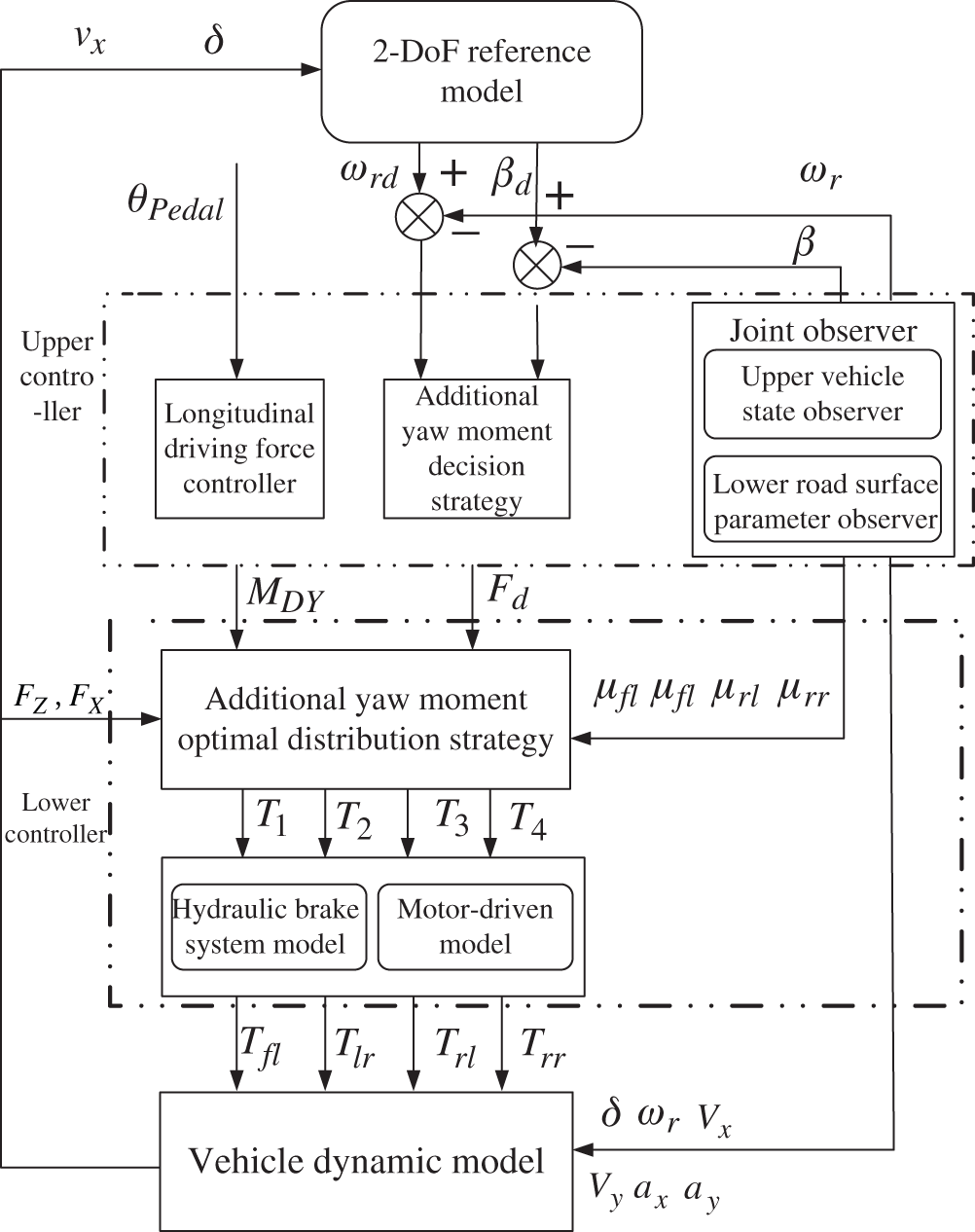
Figure 1: Structure diagram of double-layer direct yaw moment controller
The upper layer controller includes vehicle state parameter estimator model based on dual unscented Kalman filter, stability control reference model, longitudinal driving force controller and additional yaw moment decision model. The upper layer controller calculated the steady-state yaw rate
3 Joint Observer Based on the Dual Unscented Kalman Filter
Accurate acquisition of vehicle state information can improve the control effect of vehicle stability controller. The vehicle stability control strategy usually takes the yaw rate and the sideslip angle as the control targets. Yaw rate represents the vehicle’s steering dynamic characteristics and the sideslip angle reflects the vehicle’s driving trajectory. The yaw rate can be directly collected by the gyroscope. But the direct measurement of the vehicle sideslip angle is more difficult. Meanwhile, the road parameters also limit the reference yaw rate and sideslip angle. Consider the above two reasons, a joint observer of vehicle state parameters and road parameters is designed based on UKF which has good adaptability to nonlinear system.
3.1 The Dynamic Model Used in the Dual UKF Joint Observer
As shown in Fig. 3, the joint observer is constructed based on dual unscented Kalman filter based on the 3-DoF vehicle model [18–20]. The joint observer is composed of a vehicle state observer and a road parameter observer in parallel. The observation process is shown in Fig. 2. The observation process of vehicle state and road surface parameters is composed of the vehicle state time update, road parameters time update, vehicle state measurement update and the road parameters measurement update [21–23]. In every moment, vehicle state and the pavement parameters variables constitute a closed-loop feedback to each other in the process of observation, making the parameters estimation of the vehicle status and road synchronously.
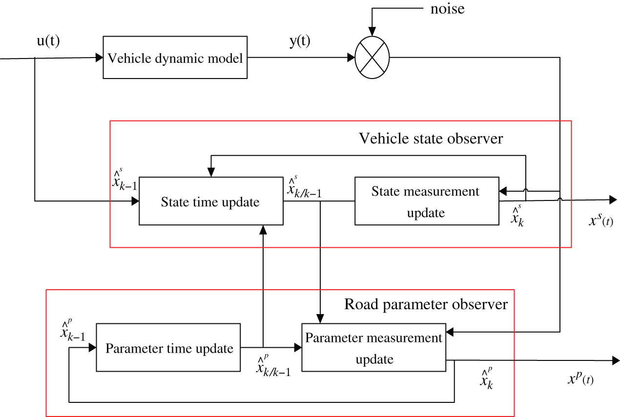
Figure 2: Flow chart of the vehicle DUKF joint observer
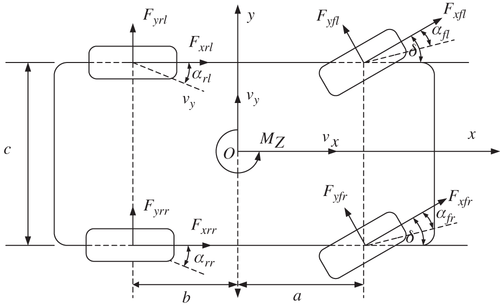
Figure 3: 3-DoF vehicle dynamic model
According to the vehicle dynamic model, the dynamic equations of longitudinal, lateral and yaw motion of the vehicle can be obtained [24]:
In the formula
According to the magic tire model [25], the longitudinal and lateral force of each wheel
where,
The vertical load of each wheel is as follows [27]:
where,
In the joint observer, vehicle state vector
The input vector
The measurement vector consists of vehicle longitudinal acceleration
According to the 3-DOF vehicle dynamics model and the magic tire model, the nonlinear vehicle state observation equation can be obtained:
In the sampling time
The vehicle sideslip angle could be calculated by the longitudinal speed and lateral speed.
The observation equation and state equation of road surface parameters observer is:
In the formula,
3.2 Construction of Dual UKF Joint Observer
(1) Establish initial 2n + 1 sigma point set
where,
Weight of sigma sampling point set’s is as follows:
(2) Vehicle state parameters time update: Calculate the one step predicted sigma points according to the state transfer function
Calculate the predicted value and covariance matrix according to the set of predicted sampling points:
where,
(3) Establish the initial sigma point set
where,
Weight of sigma sampling point set’s is as follows:
(4) Road parameters time update: calculate the one step predicted Road parameters.
Update the parameter prediction error covariance matrix.
where,
(5) Vehicle state measurement update:
Calculate covariance matrix of the vehicle state observation information:
Calculate cross covariance matrix of the vehicle state observation information:
(6) Road parameters measurement update:
Calculate covariance matrix of the road parameters observation information:
Calculate cross covariance matrix of the road parameters observation:
(7) Calculate the Kalman filter gain matric
Calculate the optimal estimation of vehicle state parameters based on the vector of vehicle state parameters
Update the covariance matrix of the vehicle state parameters error:
(8) Calculate the Kalman filter gain matric
Calculate the optimal estimation of the road parameters vector
Update covariance matrix of the road parameters error:
Let k = K + 1 repeat the above steps to realize the joint observation of vehicle state and road parameters.
4 Design of the Direct Yaw Moment Controller
4.1 Additional Yaw Moment Decision Model Based on Model Predictive Control
4.1.1 Reference Model Based on Linear 2-DoF Vehicle Model
The 2-DoF vehicle model can well describe the steady-state characteristics of the vehicle. Therefore, the yaw rate and the sideslip angle under the stable operating condition are selected as the control targets of the controller in this paper. The linear 2-DOF model is shown in Fig. 4.
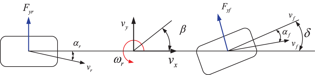
Figure 4: Linear 2-DOF reference model
The vehicle differential equation is as follows:
When vehicle is in the steady state,
When the vehicle is driving on the low adhesion coefficient road, such as rain, snow and sands, the adhesion force provided by the road adhesion condition is small, which cannot produce the high yaw rate required by the vehicle in the stable state. Therefore, when the vehicle linear 2-DOF model is selected as the reference model, the reference yaw rate and sideslip angle must be limited by the tire and road adhesion coefficient.
The upper boundary of the reference yaw rate is:
Therefore, the reference yaw rate is:
The upper bound of the reference sideslip angle must be specified. This paper adopts empirical formula (54) as the upper boundary of the sideslip angle,
Therefore, the reference sideslip angle is:
Thus, the basic control target, the reference yaw rate
4.1.2 Additional Yaw Moment Decision Based on Model Predictive Control
Adding additional yaw moment
System state equation is as follows:
where,
In order to meet the discrete control requirements of model predictive control, Euler method is used to discretization the above system space state equation [28]:
where,
Utilize the discretized state transfer equation to predict the system state in time domain P:
where,
According to the predicted system state, the corresponding output of predicted system can be obtained.
where,
The optimization objective function is shown as follows:
where,
The constraint function are as follows:
(1) Due to the motor power limit, the control input of the vehicle will be limited:
(2) Control increments also need to be limited to prevent vehicle instability caused by excessive energy fluctuation:
(3) The system output constraint
The optimal control can be obtained by solving the above quadratic programming problem:
And apply the first term in
4.2 Direct Yaw Moment Optimization Allocation Model Based on Quadratic Programming Problem
Taking the minimum tire adhesion coefficient utilization rate as the optimal allocation target of additional yaw moment [29,30]:
Introducing the following constraint conditions:
(1) Tire adhesion limit constraint:
(2) Motor system performance constraint:
where,
(3) Braking system constraints:
After torque optimization, if the torque is negative, it is necessary to apply braking torque. The braking torque should be less than the limit braking torque
This paper adopts the active set method to solve the above quadratic programming problem [31]. Active set algorithm is a very effective method to solve quadratic programming problems. It solves general constrained quadratic programming problems by solving finite equity-constrained quadratic programming problems. The active set method can be described as:
There is a method based on determining its optimal solution and corresponding multiplier at the same time, namely Lagrange function:
It can be obtained from its matrix form:
Considering the long development cycle and high cost of controller, a test platform based on experimental distributed-drive electric vehicle using A&D 5435 hardware-in-the-loop simulation system has been set up. Test on low adhesion coefficient road and joint pavement simulation conditions are conduct respectively. At the same time, the direct yaw moment controller based on “feedforward + feedback” control is designed as a comparison, so as to verify the feasibility and accuracy of the proposed stability control strategy.
5.1 Double Lane Change Test on Low Adhesion Coefficient Pavement
The target track of the double lane change condition is shown in Fig. 5. The error analysis of low adhesion coefficient double line changesimulation test is shown in Tab. 1. The road adhesion coefficient is 0.56 and the initial speed is 100 km/h. The lateral acceleration, the yaw rate and the sideslip angle under model predictive control, “feedforward + feedback” control and uncontrol are shown in Figs. 6–8, respectively.
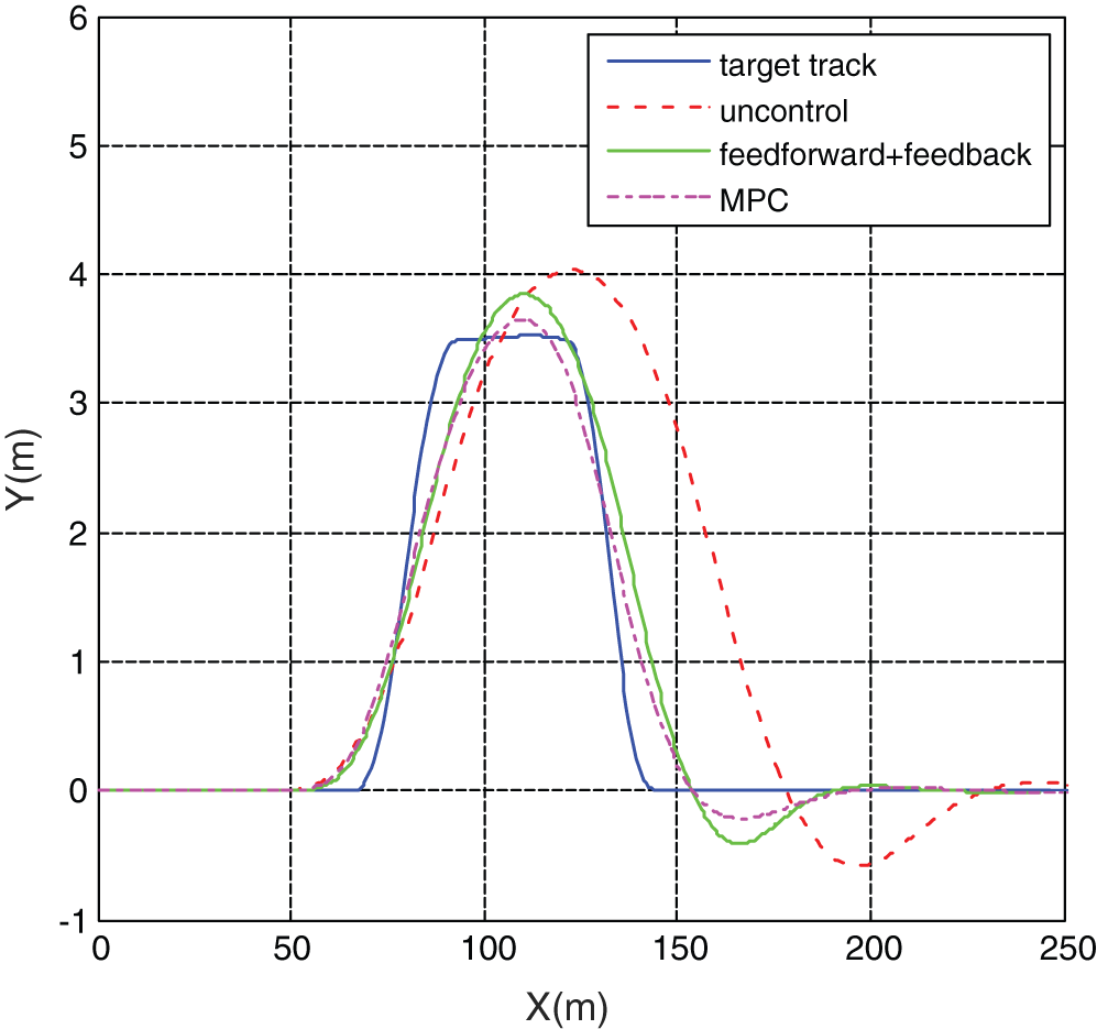
Figure 5: Vehicle track
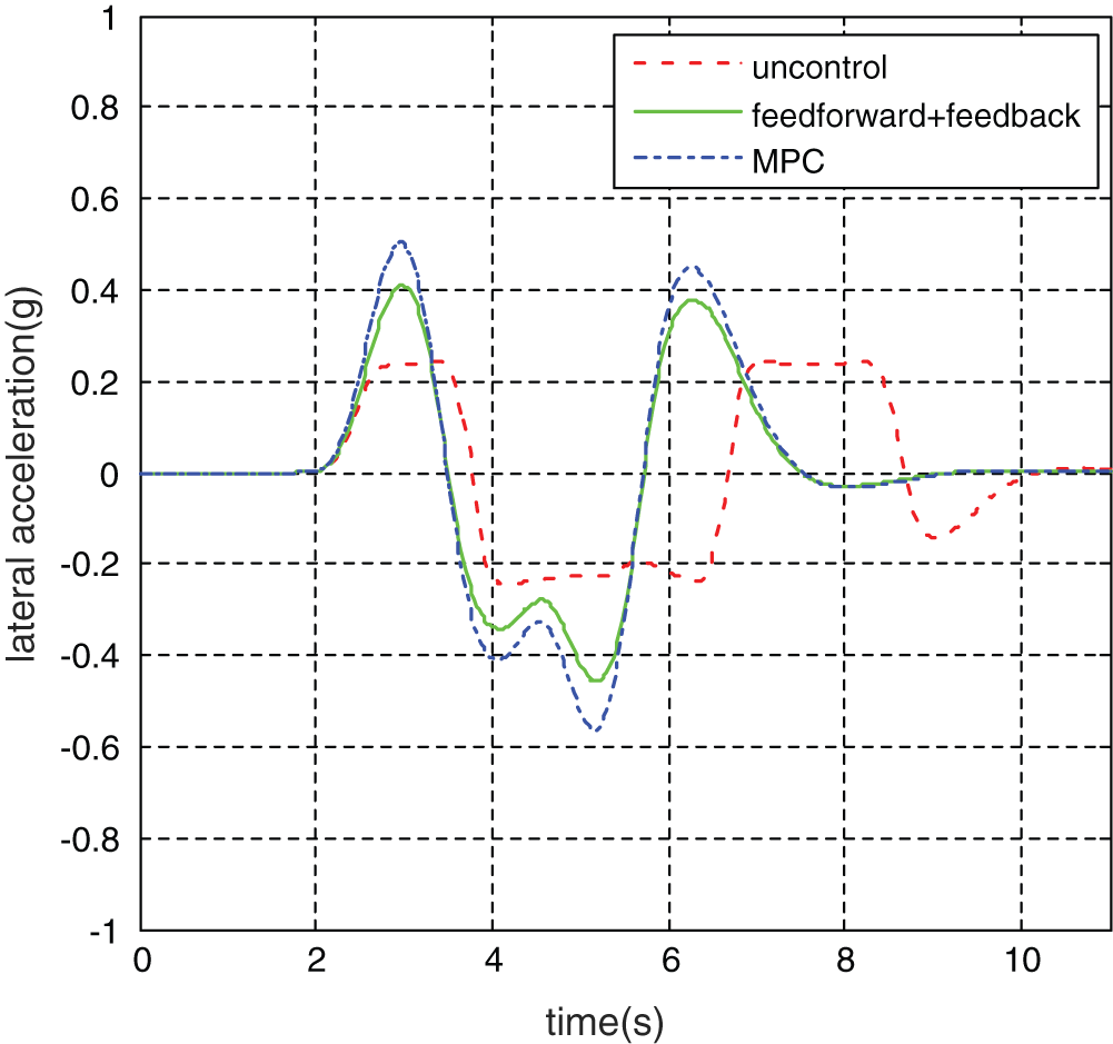
Figure 6: Vehicle lateral acceleration
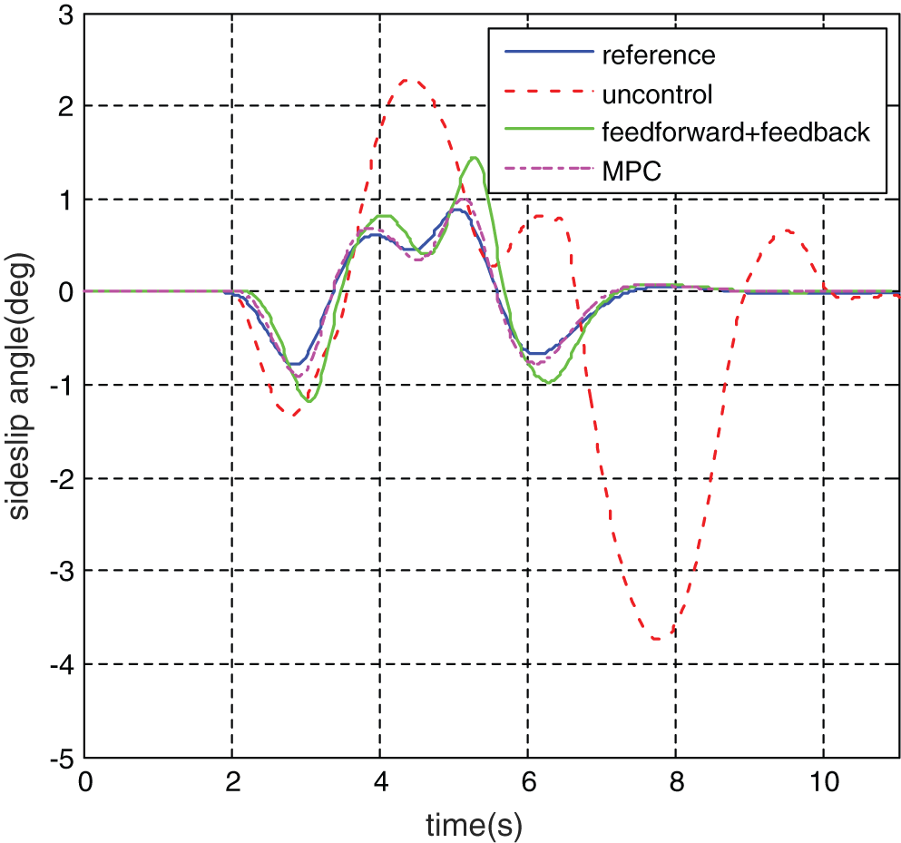
Figure 7: Vehicle sideslip angle
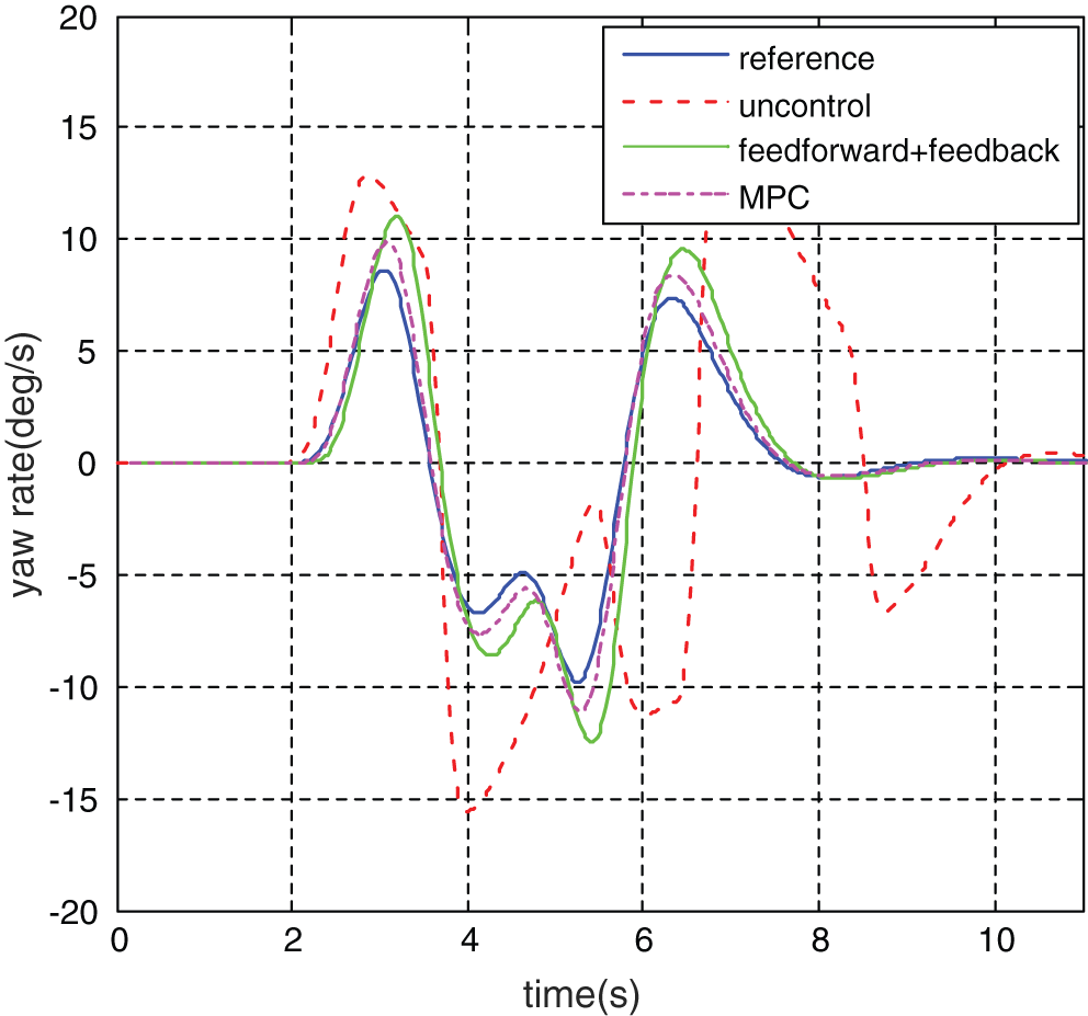
Figure 8: Vehicle yaw rate
Table 1: Error analysis table for simulation test of double line change test for low adhesion coefficient
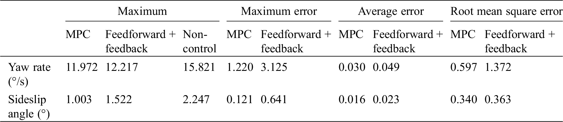
It can be seen from Fig. 5 that the vehicle track under the uncontrol deviates from the target track significantly. It can be seen from Fig. 6, under the action of MPC controller, the maximum lateral acceleration of the vehicle is only 0.4 g. Under the action of the “feedforward + feedback” control system, the lateral acceleration of the vehicle is only 0.5 g. Although the maximum lateral acceleration of the vehicle under unstable control is 0.25 g, the vehicle is already far away from the target trajectory. It can be seen from Figs. 7 and 8 that the maximum yaw rate under the uncontrol reached 15.821°/s and the maximum vehicle sideslip angle reached 2.247°. Both the MPC controller and the “feedforward + feedback” controller can well follow the change of ideal values. Under the control of MPC-based stability control system, the maximum yaw rate was 11.927°/s, which decreased by 24.6%, and the maximum sideslip angle was 1.003°, which decreased by 55.4%. Under the control of the “feedforward + feedback” stability control system, the maximum yaw rate was 12.217°/s, which decreased by 22.8%; the maximum sideslip angle was 1.522°, which decreased by 32.3%.
At the same time, according to the error analysis results, the maximum error, the mean error and the root mean square error of the vehicle yaw rate and the sideslip under MPC-based stability control system are all smaller than those under the “feedforward + feedback” controller. As can be seen from the actual driving track of the vehicle in Fig. 5, under the action of the vehicle stability control system, the vehicle travels smoothly, without dangerous conditions such as sideslip and tail swing, and the vehicle handling stability is effectively improved. Compared with the “feedforward + feedback” controller, vehicle track is much closer to the target track under the MPC controller.
Meanwhile, according to the observation data of adhesion coefficient shown in Figs. 9 and 10, the DUKF observation value rapidly converges to the true value of road adhesion coefficient within 0.2 s.
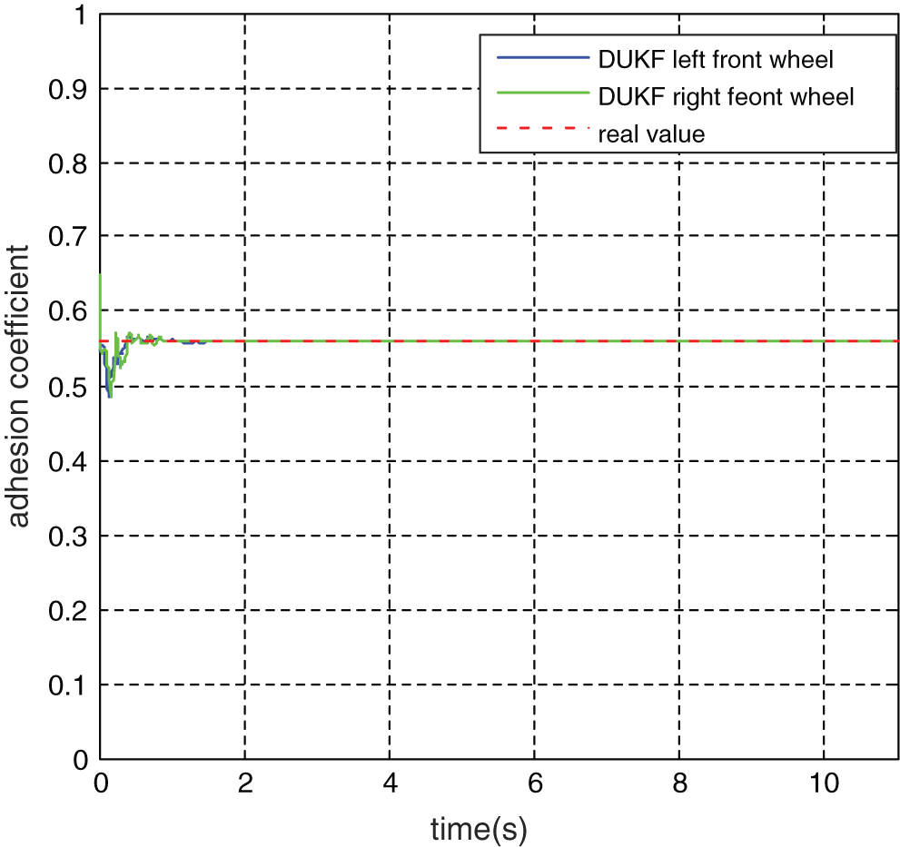
Figure 9: Observation value of adhesion coefficient of front wheel
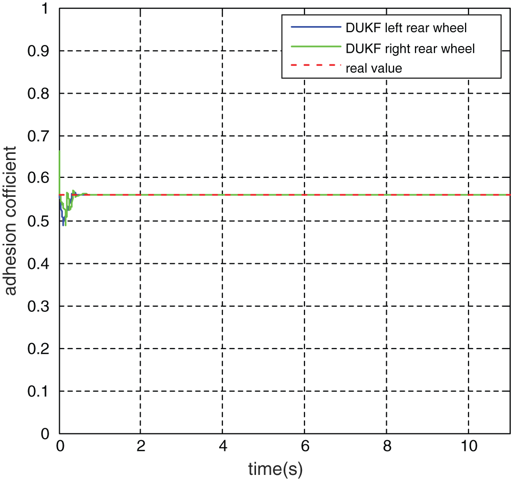
Figure 10: Observation value of adhesion coefficient of rear wheel
5.2 The Snake Test on Joint Pavement Pylon
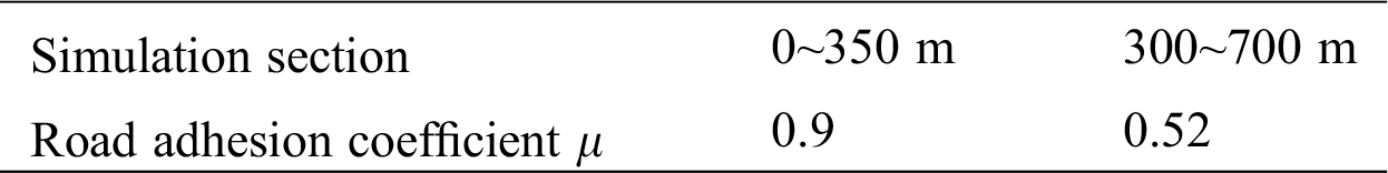
This paper selects the snake test on joint pavement pylon as test condition. The vehicle speed is 85 km/h and the road adhesion coefficient is shown in Tab. 2. The movement track of vehicle, the lateral acceleration, the yaw rate and the sideslip angle response curves of the vehicle under model predictive control, “feedforward + feedback” control and uncontrol are shown in Figs. 11–14, respectively.
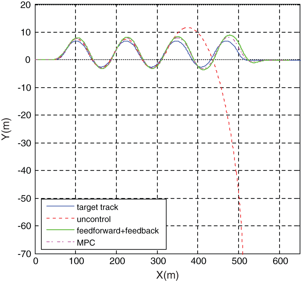
Figure 11: Vehicle track
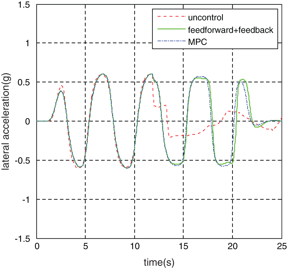
Figure 12: Vehicle lateral acceleration
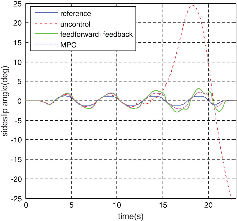
Figure 13: Vehicle sideslip angle
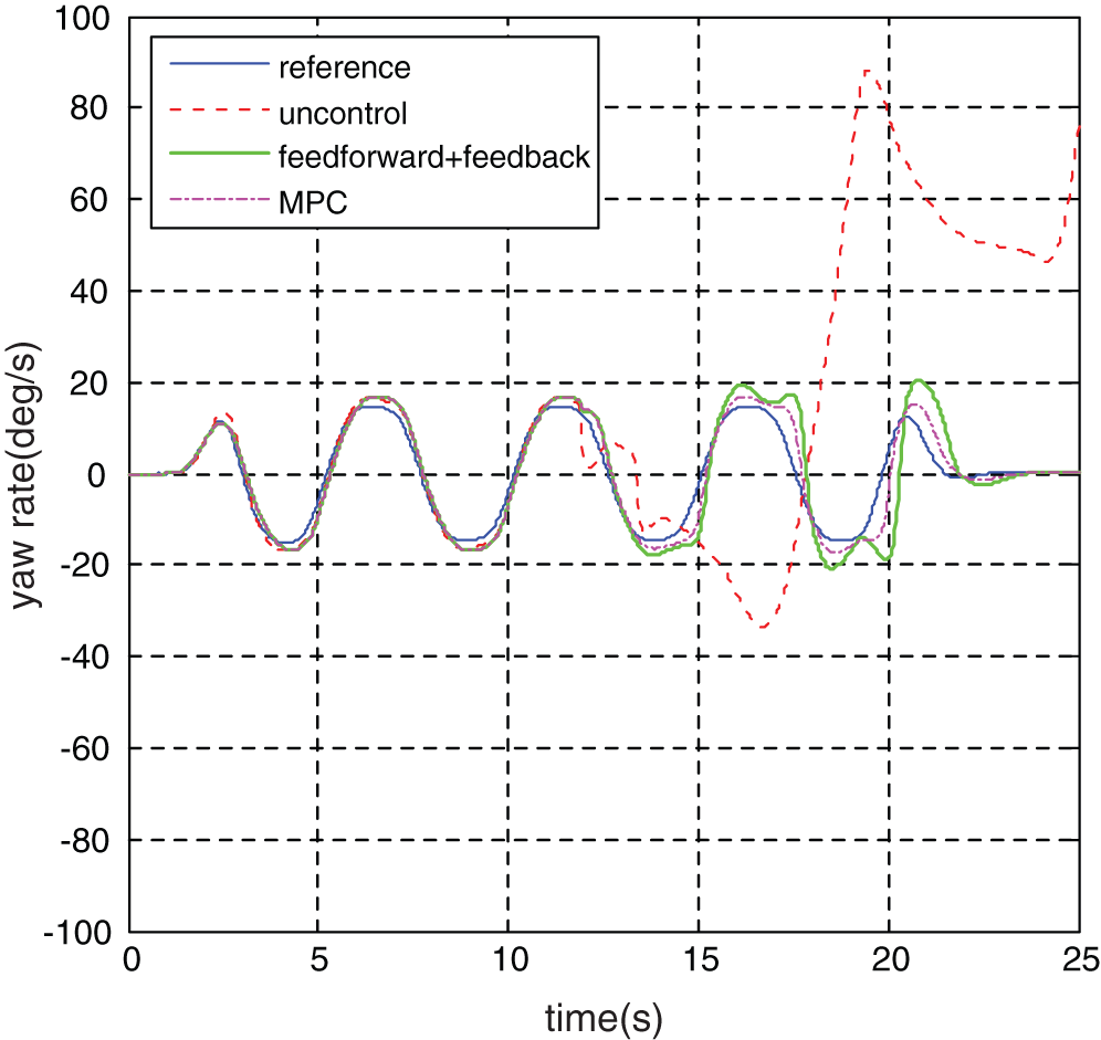
Figure 14: Vehicle yaw rate
Table 2: road section adhesion coefficient table
Error analysis was performed on the yaw rate and the sideslip angle response value after the simulation time of 12 s (road junction). The error analysis of yaw rate, sideslip angle and target value under the model prediction controller and the “feedforward + feedback” controller is shown in Tab. 3.
Table 3: Error analysis table for simulation test of the joint pavement snake test
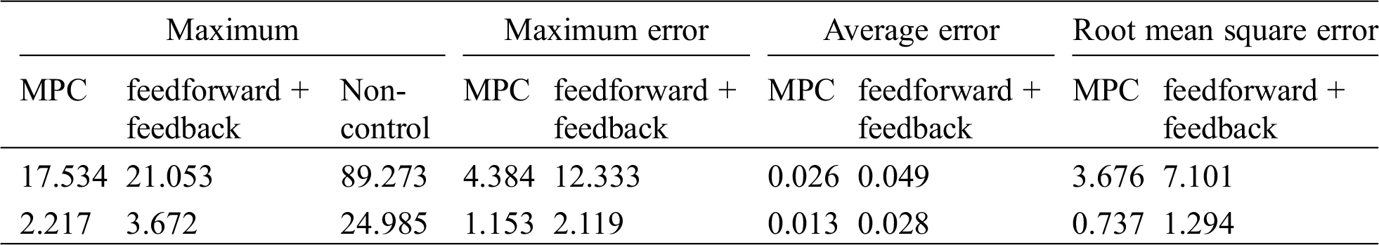
According to the Fig. 11, it can be seen that in the joint pavement without stability controller role, the vehicle begins to side slip in the longitudinal displacement of 350 m (joint pavement) and the movement track is completely away from the target track. With stability controller action, vehicles are driven to follow the target track stability and compared with the feedforward + feedback controller, vehicle track is closer to the target track under the model predictive controller. It can be seen from Figs. 13 and 14 that the maximum vehicle yaw rate reached 89.273°/s under uncontrol and the maximum sideslip angle reached 24.985°. Under the MPC stability control system, the maximum yaw rate was 17.534°/s, which decreased by 80.4%, and the maximum sideslip angle was 2.217°, which decreased by 91.1%. Under the “feedforward + feedback” stability control system, the maximum yaw rate is 21.053°/s, reducing by 76.4%, and the maximum sideslip angle is 3.672°, decreasing by 85.3.3%.
At the same time, according to the error analysis results, the maximum error, the mean error and the root mean square error of the vehicle yaw rate and the sideslip under the model predictive controller are all smaller than the error values under the “feedforward + feedback” controller. It can be seen from the Fig. 6 the actual movement track of the vehicle that vehicle running is relatively stable and no dangerous situation such as side slip, spin under the vehicle stability control system and the vehicle’s handling stability effectively improved. Compared with the feedforward + feedback controller, vehicle track is closer to the target track under the model predictive controller.
Meanwhile, according to the observation data of adhesion coefficient in Figs. 15 and 16, the DUKF observation value rapidly converges to the true value of road adhesion coefficient within 0.2 s.
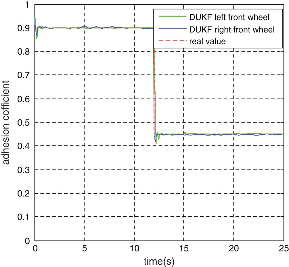
Figure 15: Observation value of adhesion coefficient of front wheel
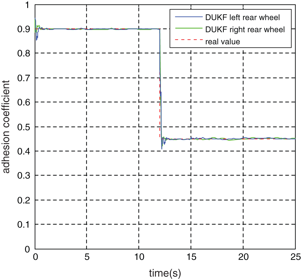
Figure 16: Observation value of adhesion coefficient of rear wheel
A double-layer structure direct yaw moment controller consisting of the additional yaw moment decision layer based on the MPC and the additional yaw moment distribution layer based on quadratic programming active set is designed. Considering the influence of road adhesion coefficient on stability control system, a joint observer of vehicle state parameters and road surface parameters is established. According to the low adhesion coefficient road and joint pavement simulation test results, the vehicle stability can get significantly improved with the vehicle stability controller based on the joint observer. In addition, compared with the “feedforward + feedback” controller, the yaw rate and sideslip angle’s response values of the distributed driven electric vehicle are closer to the steady-state value under the model prediction controller, which has more reliable control effect in terms of vehicle stability control. Future works will focus on the coordinated control of the line control system chassis.
Funding Statement: This research is funded by Youth Program of National Natural Science Foundation of China (52002034), National Key R&D Program of China (2018YFB1600701), Key Research and Development Program of Shaanxi (2020ZDLGY16-01, 2019ZDLGY15-02), Natural Science Basic Research Program of Shaanxi (2020JQ-381), Fundamental Research Funds for the Central Universities, CHD (300102220113).
Conflicts of Interest: The authors declare that they have no conflicts of interest to report regarding the present study.
1. Zhao, J., Wong, P. K., Ma, X., Xie, Z. (2017). Chassis integrated control for active suspension, active front steering and direct yaw moment systems using hierarchical strategy. Vehicle System Dynamics, 55(1), 72–103. DOI 10.1080/00423114.2016.1245424. [Google Scholar] [CrossRef]
2. Wang, C., Song, C. X., Li, J. H. (2016). Improvement of active yaw moment control based on electric-wheel vehicle ESC test platform. Fifth International Conference on Instrumentation & Measurement, 55–58. DOI 10.1109/IMCCC.2015.19. [Google Scholar] [CrossRef]
3. Zhai, L., Sun, T., Wang, J. (2016). Electronic stability control based on motor driving and braking torque distribution for a four in-wheel motor drive electric vehicle. IEEE Transactions on Vehicular Technology, 65(6), 4726–4739. DOI 10.1109/TVT.2016.2526663. [Google Scholar] [CrossRef]
4. Yager, R. R., Zadeh, L. A., Pub, K. A. (1992). An introduction to fuzzy logic applications in intelligent systems. Kluwer Academic, Netherlands. [Google Scholar]
5. Boada, B. L., Boada, M. J. L., Diaz, V. (2005). Fuzzy-logic applied to yaw moment control for vehicle stability. Vehicle System Dynamics, 43(10), 753–770. DOI 10.1080/00423110500128984. [Google Scholar] [CrossRef]
6. Zhao, J., Huang, J., Zhu, B., Shan, J. (2016). Nonlinear control of vehicle chassis planar stability based on T-S fuzzy model. SAE 2016 World Congress and Exhibition. DOI 10.4271/2016-01-0471. [Google Scholar] [CrossRef]
7. Xiao, J., Zhao, T. (2016). Overview and prospect of T-S fuzzy control. Journal of Southwest Jiaotong University, 51(3), 462–474. [Google Scholar]
8. Chilali, M., Gahinet, P. (1996). H ∞ design with pole placement constraints: An LMI approach. Proceedings of the 49th IEEE Conference on Decision and Control, 553(3), 358–367. [Google Scholar]
9. Yin, G., Chen, N., Li, P. (2007). Improving handling stability performance of four-wheel steering vehicle via μ-synthesis robust control. IEEE Transactions on Vehicular Technology, 56(5), 2432–2439. DOI 10.1109/TVT.2007.899941. [Google Scholar] [CrossRef]
10. Hang, P., Chen, X. B., Fang, S. D., Luo, F. M. (2017). Robust control of a four-wheel-independent-steering electric vehicle for path tracking. SAE International Journal of Vehicle Dynamics, Stability, and NVH, 1(2), 307–316. DOI 10.4271/2017-01-1584. [Google Scholar] [CrossRef]
11. Demirci, M., Gokasan, M. (2013). Adaptive optimal control allocation using Lagrangian neural networks for stability control of a 4WS–4WD electric vehicle. Transactions of the Institute of Measurement and Control, 35(8), 1139–1151. DOI 10.1177/0142331213490597. [Google Scholar] [CrossRef]
12. Chen, J., Chen, N., Yin, G., Guan, Y. (2010). Sliding-mode robust control for 4WS vehicle based on non-linear characteristic. Journal of Southeast University (Natural Science Edition), 40(5), 969–972. [Google Scholar]
13. Wang, Z. P., Wang, Y. C., Zhang, L., Liu, M. C. (2017). Vehicle stability enhancement through hierarchical control for a four-wheel-independently-actuated electric vehicle. Energies, 10(7), 947–992. DOI 10.3390/en10070947. [Google Scholar] [CrossRef]
14. Barbarisi, O., Palmieri, G., Scala, S., Glielmo, L. (2009). LTV-MPC for yaw rate control and side slip control with dynamically constrained differential braking. European Journal of Control, 15(3–4), 468–479. DOI 10.3166/ejc.15.468-479. [Google Scholar] [CrossRef]
15. Falcone, P., Eric Tseng, H., Borrelli, F., Asgari, J., Hrovat, D. (2008). MPC-based yaw and lateral stabilisation via active front steering and braking. Vehicle System Dynamics, 46(sup1), 611–628. DOI 10.1080/00423110802018297. [Google Scholar] [CrossRef]
16. Jalali, M., Khajepour, A., Chen, S. K., Litkouhi, B. (2016). Integrated stability and traction control for electric vehicles using model predictive control. Control Engineering Practice, 54, 256–266. DOI 10.1016/j.conengprac.2016.06.005. [Google Scholar] [CrossRef]
17. Guo, N., Lenzo, B., Zhang, X., Zou, Y., Zhang, T. (2020). A real-time nonlinear model predictive controller for yaw motion optimization of distributed drive electric vehicles. IEEE Transactions on Vehicular Technology, 69(5), 4935–4946. DOI 10.1109/TVT.2020.3039339. [Google Scholar] [CrossRef]
18. Chen, T., Xu, X., Chen, L., Jiang, H., Cai, Y. et al. (2018). Estimation of longitudinal force, lateral vehicle speed and yaw rate for four-wheel independent driven electric vehicles. Mechanical Systems & Signal Processing, 101, 377–388. DOI 10.1016/j.ymssp.2017.08.041. [Google Scholar] [CrossRef]
19. Wang, Z. P., Xue, X., Wang, Y. C. (2018). State parameter estimation of distributed drive electric vehicle based on adaptive unscented Kalman filter. Beijing Ligong Daxue Xuebao/Transaction of Beijing Institute of Technology, 38(7), 698–702. [Google Scholar]
20. Huang, X. P. (2015). Principle and application of Kalman filter. China: Publishing House of Electronics Industry. [Google Scholar]
21. Du, H., Lam, J., Cheung, K. C., Li, W., Zhang, N. (2015). Side-slip angle estimation and stability control for a vehicle with a non-linear tyre model and a varying speed. Proceedings of the Institution of Mechanical Engineers Part D Journal of Automobile Engineering, 229(4), 486–505. DOI 10.1177/0954407014547239. [Google Scholar] [CrossRef]
22. Yu, A., Liu, Y., Zhu, J., Dong, Z. (2015). An improved dual unscented Kalman filter for state and parameter estimation. Asian Journal of Control, 18(4), 1427–1440. DOI 10.1002/asjc.1229. [Google Scholar] [CrossRef]
23. Jin, X. J., Yang, J. P., Yin, G. D., Wang, J. X., Chen, N. et al. (2019). Combined state and parameter observation of distributed drive electric vehicle via dual unscented Kalman filter. Journal of Mechanical Engineering, 55(22), 93–102. [Google Scholar]
24. Wang, Z. P., Zhu, J. J., Zhang, L., Wang, Y. C. (2018). Automotive ABS/DYC coordinated control under complex driving conditions. IEEE Access, 6, 32769–32779. [Google Scholar]
25. Nam, K. (2012). Lateral stability control of in-wheel-motor-driven electric vehicles based on sideslip angle estimation using lateral tire force sensors. IEEE Transactions on Vehicular Technology, 61(5), 1972–1985. DOI 10.1109/TVT.2012.2191627. [Google Scholar] [CrossRef]
26. Shuai, Z., Zhang, H., Wang, J., Li, J., Ouyang, M. (2014). Combined AFS and DYC control of four-wheel-independent-drive electric vehicles over can network with time-varying delays. IEEE Transactions on Vehicular Technology, 63(2), 591–602. DOI 10.1109/TVT.2013.2279843. [Google Scholar] [CrossRef]
27. Zhao, L. H., Liu, Z. Y., Chen, H. (2011). Design of a nonlinear observer for vehicle velocity estimation and experiments. IEEE Transactions on Control Systems Technology, 19(3), 664–672. DOI 10.1109/TCST.2010.2043104. [Google Scholar] [CrossRef]
28. Zhao, X., Wang, Z. P., Jia, H. H. (2015). Comparison and analysis of discretization methods for continuous systems. Industry and Information Technology Education, 10, 71–82. [Google Scholar]
29. Zou, G., Luo, Y., Li, K. (2009). 4WD vehicle DYC based on tire longitudinal forces optimization distribution. Transactions of the Chinese Society for Agricultural Machinery. DOI 10.1109/CLEOE-EQEC.2009.5194697. [Google Scholar] [CrossRef]
30. Sun, W. Y. (2004). Optimization method. China: Higher Education Press. [Google Scholar]
31. Yi, Y. H. (2008). A modified active-set algorithm for quadratic programming (Master’s Thesis). Jiangxi Normal University, Nanchang. [Google Scholar]
 | This work is licensed under a Creative Commons Attribution 4.0 International License, which permits unrestricted use, distribution, and reproduction in any medium, provided the original work is properly cited. |