Energy Engineering

DOI: 10.32604/EE.2021.014724

ARTICLE

Application of Model Predictive Control Based on Kalman Filter in Solar Collector Field of Solar Thermal Power Generation

Xiaojuan Lu and Zeping Liang*

Lanzhou Jiaotong University, Lanzhou, 730070, China
*Corresponding Author: Zeping Liang. Email: 18368914525@163.com
Received: 24 October 2020; Accepted: 14 December 2020

1  Introduction

As an environmentally and widely available renewable energy, solar energy has broad development prospects. At present, many countries use solar energy to generate electricity by establishing photovoltaic power stations or solar thermal power stations. The focused solar thermal power station focuses the solar energy through the collector, and then heats the heat transfer working medium inside the collector. The heated heat transfer working fluid generates steam through the heat exchanger and drives the steam turbine to generate electricity. In order to ensure stable power output, the outlet temperature of the solar thermal field must be able to maintain the set operating point. Due to the non-linearity, complexity, delay and strong random interference characteristics of the solar heat collection field, the control of the outlet temperature of the heat transfer working fluid in the heat collection loop has become a hot and difficult problem in the research field of solar thermal power generation.

This paper studies solar power plants with linear Fresnel (LF) collectors. The LF collector is an improvement and simplification of the trough collector. Its heat collection system is mainly composed of a condenser and a glass-metal vacuum heat sink. The concentrator can be regarded as the linear segmentation discretization of the parabolic trough reflector, it reflects the incident light from the sun and gathers it on the focal line of the linear strip mirror. The heat sink is installed above the focal line and heating the heat transfer fluid, and finally realize the conversion of solar energy to thermal energy [1]. The LF collector field is affected by a variety of interference sources. At present, the main considerations are the change of solar radiation intensity, the change of ambient temperature, the fluctuation of the inlet molten salt temperature and the influence of the molten salt flow rate on the outlet salt temperature of the collector loop. Among them, the intensity of solar radiation is the most important interference, because scattered clouds may produce strong changes throughout the day. Therefore, the main purpose of the LF collector field control system is to maintain the temperature of the working fluid at the outlet of the collector loop at a desired level [2].

In response to the problem of temperature control of LF collector field, many scholars at home and abroad have done a lot of research, including traditional PID control, model-based predictive control (MBPC) [3], adaptive control, internal model control(IMC), and nonlinear control [4,5] etc. In Lima et al. [6], a filter dynamic matrix control (FDMC) is used to control the output temperature of a solar collector field of the desalination plant. In the filter dynamic matrix control, a filter is used in the prediction error, which can improve the robustness and anti-interference characteristics of the original algorithm. In Brus et al. [7], a generalized predictive control algorithm with feedforward compensation is proposed, which uses feedforward control to compensate for disturbances and the strong robustness of predictive control to improve the tracking effect of predictive control on collector outlet oil temperature. In Xu et al. [8], according to the dynamic mathematical model of a parabolic trough solar collector loop, using direct normal irradiation, inlet oil temperature of the collector and ambient temperature as disturbances, PID controller and IMC are designed. The result shows that IMC is more effective. In Lu et al. [9], an adaptive prediction model of solar collector was established based on the measured data. The author adopting a switching strategy based on the minimum cumulative error, the optimal control model was selected online, and an active fault tolerant sliding mode predictive controller was designed, which improved the tracking accuracy and robustness of the system. The above controllers are all control strategies for suppressing general interference, and lack of suppression strategies for unmeasured (unmodeled) interference. Traditional predictive control and robust control have poor control effects on unmeasured disturbances of objects with large inertia and large delay.

Since the factors that affect the overall efficiency such as direct solar radiation, specular reflectance and metal absorptance can only be measured locally, and other unmodeled factors such as wind speed, it is necessary to consider these interferences in the process of controlling the salt temperature at the outlet of the collector to improve the control effect [10]. In this paper, solar radiation intensity, ambient temperature, and inlet molten salt temperature are used as measurable disturbances, and a DMC controller is designed to control the outlet molten salt temperature of the collector by adjusting the working fluid flow. In order to solve the problem of the deterioration of DMC control performance caused by excessive solar radiation intensity fluctuations and unmeasured disturbances, this paper expand on the basis of the classic DMC algorithm prediction model. A steady-state Kalman filter is design to estimate unmeasured interference, state variables and future output. And it also is used to improve the system’s ability to suppress unmeasured interference. This paper provides reference for actual operation control of domestic LF power station.

2  Mathematical Model of LF Collector Field

The Dacheng Dunhuang LF Power Station is currently composed of a heat collection field, a heat storage system and a power generation system. The heat collecting field uses binary molten salt as the heat transfer medium, with a total of 80 parallel circuits and a total mirror area of 1.27 million m2.

2.1 Distributed Parameter Model

After general simplification and assumptions, the distributed LF collector field can be described by a distributed parameter model about temperature. This distributed parameter model includes the energy balance equation of the metal heat absorption tube and the energy balance equation of the heat transfer fluid in the heat absorption tube [11]:

ρmcmAm∂Tm∂t(t,x)=ηGI(t)−hfL[Tm(t,x)−Tf(t,x)]−haG[Tm(t,x)−Ta(t)] (1)

hfL[Tm(t,x)−Tf(t,x)]=ρfcfAf∂Tf∂t(t,x)+ρfcfv(t)∂Tf∂x(t,x) (2)

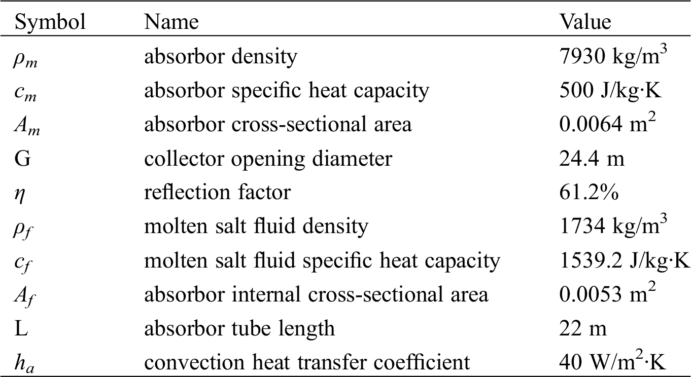
where I is the solar radiation intensity; hf is the convective heat transfer coefficient between the molten salt and the absorbor tube; Tm is the wall temperature of the metal absorbor tube; Ta is the ambient temperature; Tf is the temperature of molten salt fluid; v is the molten salt mass flow in the solar collector field. The descriptions and values of the other parameters are shown in Tab. 1.

Since the heat transfer effect between the metal absorbor tube and the heat transfer fluid is good, it is assumed that the metal absorbor tube temperature is equal to the heat transfer fluid temperature [12], That is, Tm(t,x) = Tf(t,x), according to Eqs. (1) and (2), the simplified energy balance equation is shown in Eq. (3):

(Cm+Cf)dTfo(t)dt=ηGI(t)−ρfcfv(t−dc)Tfo(t)−Tfi(t)Δx−haG[Tfo(t)−Ta(t)] (3)

where, Tfi is the inlet molten salt temperature, Tfo is the outlet molten salt temperature, Cm=ρmcmAm , Cf=ρfcfAf , Δx=L .

Table 1: Parameter of the process

2.2 Linearization and Discretization Model

Since linear discrete model is used in the predictive control algorithm, it is necessary to linearize and discretize the energy balance equation given in Eq. (3).The outlet molten salt temperature of collector field is a function of solar radiation intensity, ambient temperature, inlet molten salt temperature and molten salt mass flow. Therefore, Eq. (3) can be expressed as Eq. (4):

dTfodt=f(I(t),Ta(t),Tfi(t),Tfo(t),v(t)) (4)

Using Taylor linear approximation, select an appropriate operating point to linearize the model and the result is shown in Eq. (5):

d(ΔTfo)dt=aΔI+bΔTa+cΔTfi+dΔTfo+eΔv (5)

Then use the differential approximation of the derivative to discretize the Eq. (5). The discretization result is shown in Eq. (6):

ΔTfo(k)=(1+dTs)ΔTfo(k−1)+aTsΔI(k−1)+bTsΔTa(k−1)+cTsΔTfi(k−1)+eTsΔv(k−1−dz) (6)

The linearized and discretized transfer function is shown in Eqs. (7)–(10):

ΔTfo(z)Δv(z)=eTsz−(1+dTs)sz−dz (7)

ΔTfo(z)ΔI(z)=aTsz−(1+dTs) (8)

ΔTfo(z)ΔTa(z)=bTsz−(1+dTs) (9)

ΔTfo(z)ΔTfi(z)=cTsz−(1+dTs) (10)

where, a=ηGCm+Cf , b=haGCm+Cf , c=ρfcfv¯L(Cm+Cf) , d=−ρfcfv¯+haGLL(Cm+Cf) , e=−ρfcf(T¯fo−T¯fi)L(Cm+Cf) , v¯ , T¯fo , T¯fi represent the working point of variables v , Tfo , Tfi .

3  Dynamic Matrix Control Based on Steady-State Kalman Filter

In order to solve the control object with large inertia, large delay and nonlinearity such as solar thermal field, so that it still has good control effect in the case of model mismatch, this paper proposes a DMC predictive control with steady-state Kalman filter algorithm (KFDMC). The KFDMC control structure diagram of the LF collector is shown in Fig. 1. The collector control system is mainly composed of the collector model, the open loop prediction module, the steady state Kalman filter and the dynamic control module. Solar radiation intensity, ambient temperature, inlet molten salt temperature and other unmeasurable disturbances are not necessary to be controlled in the input of collector model.The input needs to be controlled is the temperature and mass flow of molten salt at the collector outlet. The The KFDMC controller can compensate for unstable control effects caused by time-varying and random disturbances in the heat collection field through the open-loop prediction module, steady-state Kalman filter and dynamic control module, and has relatively low requirements on the mathematical model of the controlled system [12].

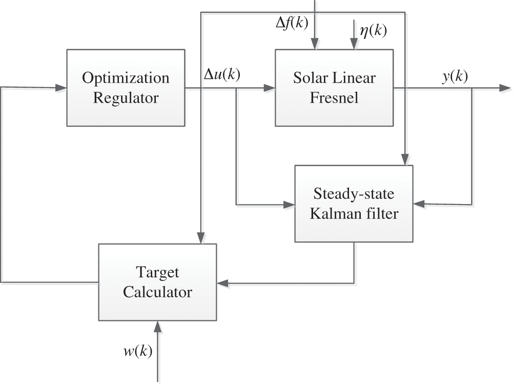
Figure 1: KFDMC structure

According to the linear collector model established in 2.2, the KFDMC controller was designed. Use Eq. (7) to obtain the step response model of input and output, and use Eqs. (8)–(10) to obtain the step response model of measurable disturbance. Among them, y(t) is the measured value of the outlet molten salt temperature, that is Tfo; u(t) is the molten salt mass flow, that is v; f(t) is the measurable disturbance that affects the outlet molten salt temperature of the collector, including solar radiation intensity I, ambient temperature Ta, and inlet salt temperature Tfi; η(t) is the unmeasured interference that affects the salt temperature at the outlet of the collector, including unmodeled interference such as local measurement and wind speed.

KFDMC algorithm is a model-based control algorithm and applies the principle of online optimization. The online calculation of KFDMC consists of an initialization module and a real-time control module. The initialization module detects the actual output y of the object in the first step of operation and sets it to the predicted initial value ys(i) , i = 1,…,n. From the second step, it is transferred to the real-time control module, and the online calculation process at each sampling moment is shown in the Fig. 2. Due to uncertain factors such as actual model mismatch, unmeasured (unmodeled) interference, noise, etc., the actual output at time k is y(k)≠yfr(k) . In order to eliminate the interference of unmeasurable disturbances and obtain the optimal estimate, Kalman filtering is used to estimate the future output [13], get the open-loop dynamic prediction value yol(i) and prediction error ε(i) . The initial predicted value ys(i) of the next time is obtained by the shift operation of ys(i) at the current time. Use ys(i) to replace the actual output y, and use the rolling optimization method to obtain the control increment Δu , We have got the measurable disturbance Δf , finally, the free predicted value yfr(i) at k+1 time can be obtained and enter the next cycle.

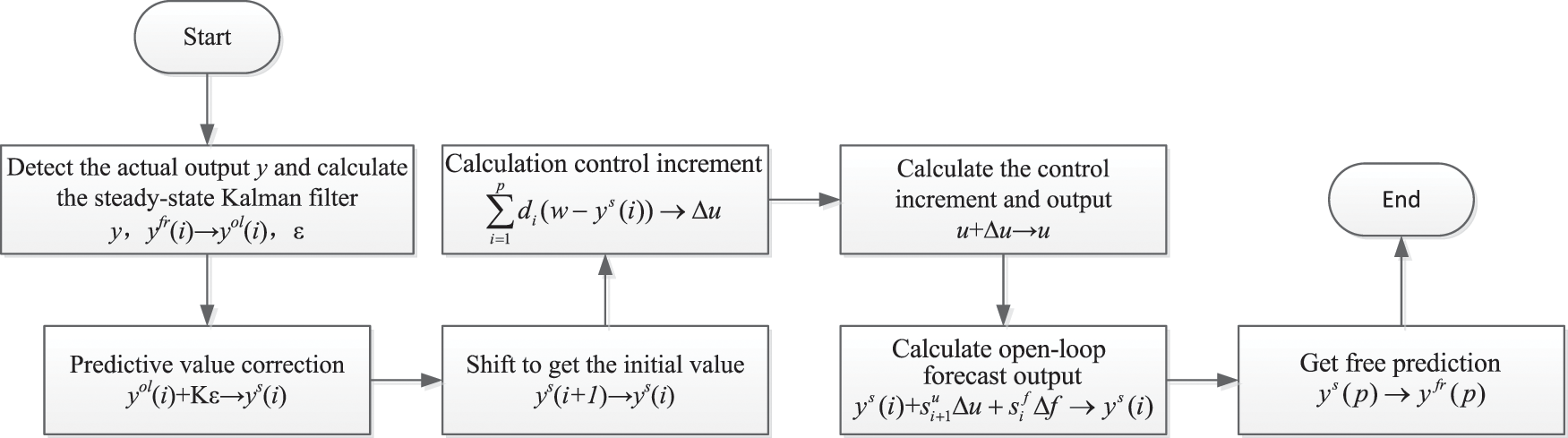
Figure 2: KFDMC algorithm flowchart

3.1 Steady State Prediction Module

The DMC system uses the step response of the system to calculate the output predicted value. For the SISO system, the open-loop prediction output at time k is [14,15]:

ys(k)=∑i=1n−1siuΔu(k−i)+snuu(k−n)+∑i=1n−1sifΔf(k−i)+snff(k−n) (11)

where, siu , siu are the step response coefficients corresponding to u and f respectively, satisfy the condition sn+iu=snu , sn+if=snf , ∀i≥0 .

At time k, Δu(k) has not been obtained, assuming that Δf(k) has been obtained. Let yfr(k+p|k) be the predicted value of ys(k+p|k) in the condition of Δu(k+i−1|k)=0 , 1≤i≤p and Δf(k+i)=0 , 1≤i≤p−1 ,which is called the free predicted value. And yfr(k+i|k)=yfr(k+n|k) , ∀i≥n . Use Eq. (11) to make predictions to obtain free predictive values, as shown in Eq. (12):

yfr(k+p|k)−yfr(k+p|k−1)=sp+1uΔu(k−1)+spfΔf(k) (12)

Satisfy the condition: yfr(k|k)=ys(k) .

Then it is obtained by Eq. (12):

Y~n+1fr(k+1)=M{Y~n+1fr(k)+[0Snu]Δu(k)}+[0Snf]Δf(k+1) (13)

where, Snu=[s1u,...,snu]T , Snf=[s1f,...,snf]T , Y~n+1fr(k|k)≜[yfr(k|k)yfr(k+1|k)⋮yfr(k+n|k)]≜[yfr(k|k)Ynfr(k)]=[Y~nfr(k)yfr(k+n|k)] , M=[0I0[0⋯0I]] .

3.2 Design of Steady-State Kalman Filter

Since the step model does not include wind speed and other unmeasured (unmodeled) factors that interfere with stable controlled variables, it will inevitably lead to tracking errors. In order to eliminate errors and suppress unmeasured interference, a steady-state Kalman filter is introduced into the DMC algorithm to realize the estimation of system state variables containing unmeasured interference.

To design a steady-state Kalman filter, consider the following state-space model to describe the dynamic system:

Y~n+1fr(k+1)=M{Y~n+1fr(k)+[0Snu]Δu(k)}+[0Snf]Δf(k+1)+η(k) (14)

ys(k)=HY~n+1fr(k)+ξ(k) (15)

where, H=[I0⋯0] .

Assume 2.1 η(k) and ξ(k) are uncorrelated white noises whose variance matrix is Q and R. E[η(k)]=0,E[ξ(k)]=0 , E[η(k)ηT(j)]=Qκkj,E[ξ(k)ξT(j)]=Rκkj , E[η(k)ξT(j)]=0,∀k,j .

where, κkk=1 , and k≠j 时, κkj=0 .

Assume 2.2 x(0) is not related to η(k) and η(k) , and E[x(0)]=μ0 , E[(x(0)−μ0)(x(0)−μ0)T]=P0 .

Assume 2.3 u(k)∈Rm is a known control input, which can be a known deterministic (non-random) input, or feedback control, that is, u(k) is a linear function of {y(k),y(k−1),...;u(k−1),u(k−2),...} .

Theorem 2.1 (Steady state Klaman filter) System Eqs. (14)–(15) under assumptions 2.1–2.3, the steady state Kalman filter is [16]:

Y~n+1ol(k|k)=M{Y~n+1ol(k−1|k−1)+[0Snu]Δu(k−1)}+[0Snf]Δf(k)+Kε(k) (16)

ε(k)=ys(k)−yol(k|k−1)−s1uΔu(k−1) (17)

K=ΣHT(HΣHT+Qy)−1 (18)

Σ=M[Σ−ΣHT(HΣHT+Qy)−1HΣ]MT+Ry (19)

Call K the Kalman filter gain.

where, Y~n+1ol(k|k)≜[yol(k|k)yol(k+1|k)⋮yol(k+n|k)]≜[yol(k|k)Ynol(k)] , K=[K0K1] .

ε(k) reflects the influence of uncertain factors not included in the step response model on the stable controlled variable, which is called prediction error. The introduction of the ε(k) makes the system a closed-loop negative feedback system, which improves the system’s ability to suppress undetectable interference. Σ is the only positive definite solution of the Riccati equation, Qy and Ry is an adjustable parameter.

From Eq. (16), the open-loop predictive output module is as follows:

Ynol(k|k)=M{Ynol(k−1|k−1)+SnuΔu(k−1)}+SnfΔf(k)+K1ε(k) (20)

3.3 Dynamic Control Module

Take modeling time domain n, forecast time domain p, control time domain m, and satisfy m≤p≤n+m . At each time k, if Ynol(k|k) is known, pol(k|k)=[yol(k+1|k),...,yol(k+p|k)]T can be obtained. When p > n, yol(k+j|k)=yol(k+n|k) , j > n. And the predicted value already includes the influence of interference and feedback correction of prediction errors. According to Eqs. (11) and (12), the closed-loop prediction equation is obtained as shown in Eq. (21):

Yp(k|k)=Ypol(k|k)+SuΔu~(k|k) (21)

where, Su=[s1u0s2us1u⋮⋮⋱spusp−1u⋯sp−m+1u] , Δu~(k|k)=[Δu(k|k),Δu(k+1|k),⋯,Δu(k+m−1|k)]T , Yp(k)=[y(k+1|k),y(k+2|k),⋯,y(k+p|k)]T .

The optimization process of predictive control is repeated online, and the optimization criterion is minimized at each moment to achieve optimization, that is, rolling optimization. Choose the optimal objective function as follows:

J(k)=∑i=1p||w(k+i)−y(k+i|k)||Q2+∑j=1m||Δu(k+j−1|k)||R2 (22)

s.t.: ymin≤y(k+i|k)≤ymax , i=1,...,p

umin≤u(k+j|k)+Δu(k+j|k)≤umax , j=0,...,m−1

The molten salt fluid selected in the project is composed of 60% NaNO3 and 40% KNO3. Its melting point is about 220°C, and its vaporization point is about 600°C. The expected operating temperature range is 290°C to 550°C. The molten salt flow rate varies from 0 kg/s to 50 kg/s. From Eqs. (7)–(10), it is known that the range of the variable affects the parameters of the transfer function of the linearized model. Therefore, the expected range of differences between variables will be used to calculate uncertainty. Considering the range of variables, take the operating point parameter values as: v¯=31.29kg/s , T¯fo=290∘C , T¯fi=550∘C .

According to the necessary conditions for taking extreme values ∂J/∂Δu~=0 , we can get:

Δu~(k)=(SuTQSu+R)−1SuTQ[Wp(k)−Yp(k)] (23)

where, DT=(SuTQSu+R)−1SuTQ is the control vector, Q=diag(q1⋯qp) and R=diag(r1⋯rm) are the error weight matrix and the control weight matrix, respectively. Wp(k) is the desired output sequence, and Wp(k)=[w(k+1),w(k+2),⋯,w(k+p)]T .

So far, DMC has obtained the optimal control variable matrix that should be applied at each time, but DMC uses rolling optimization. At each time k, DMC only selects the first parameter in the optimal control variable matrix as the actual application. The amount of control, that is:

Δu(k)=[10⋯0]Δu~(k) (24)

4  Simulation Experiment Analysis

4.1 Collector Model Verification

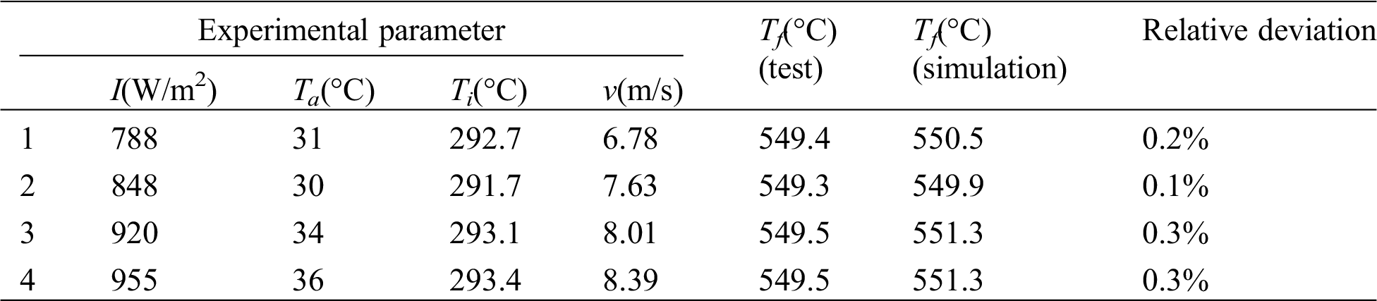
The collector model verification is carried out by comparing with the actual operating data of Dacheng Dunhuang Linear Fresnel Power Plant. Use the solar radiation intensity I, the ambient temperature Ta, the collector molten salt inlet temperature Tfi and the molten salt flow rate v as input to the collector model established above, and simulate the model. The comparison between the steady-state simulation results of the collector and the experimental data of the Dacheng Dunhuang LF Power Station is shown in Tab. 2, the relative errors of the collector outlet temperature and the experimentally measured value of the collector outlet temperature are 0.2%, 0.1%, 0.3%, 0.3%, respectively. The simulation results are basically consistent with the experimental results, which proves that the steady-state results of the model are correct and reasonable.

Table 2: Comparison table of steady-state simulation results and experimental results of collectors

4.2 KFDMC Control System Simulation Experiment

In this section, two different weather conditions are used to analyze the performance of the controller. Take the sampling time Ts = 1 min, use Eq. (7) to obtain the input and output step sampling sequence {siu,i=1,2,...,n} , and use Eqs. (8)–(10) to get the step sampling sequence {sif,i=1,2,...,n} with measurable disturbance. Assume that the unmeasurable disturbance η(k) and measurement noise ξ(k) are independent Gaussian white noise with variances of 0.8 and 1.

The simulation data of the measurable disturbances I, Ta and Tfi used to simulate a day with clear weather and no cloud cover is shown in Fig. 3. The fluctuation of solar radiation intensity is small, when the model mismatch problem caused by unmeasured disturbance is not considered, both PID controller and DMC controller can achieve better control effect and can effectively suppress radiation interference, at the same time, DMC controller has smaller overshoot and the same rise time. The simulation results are shown in Fig. 4.

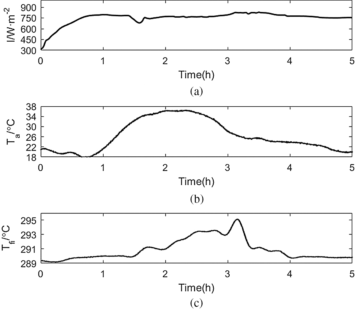
Figure 3: Simulation and disturbance data for a clear day (a) Direct normal irradiation (b) Ambient temperature (c) Inlet molten salt temperature of collector field

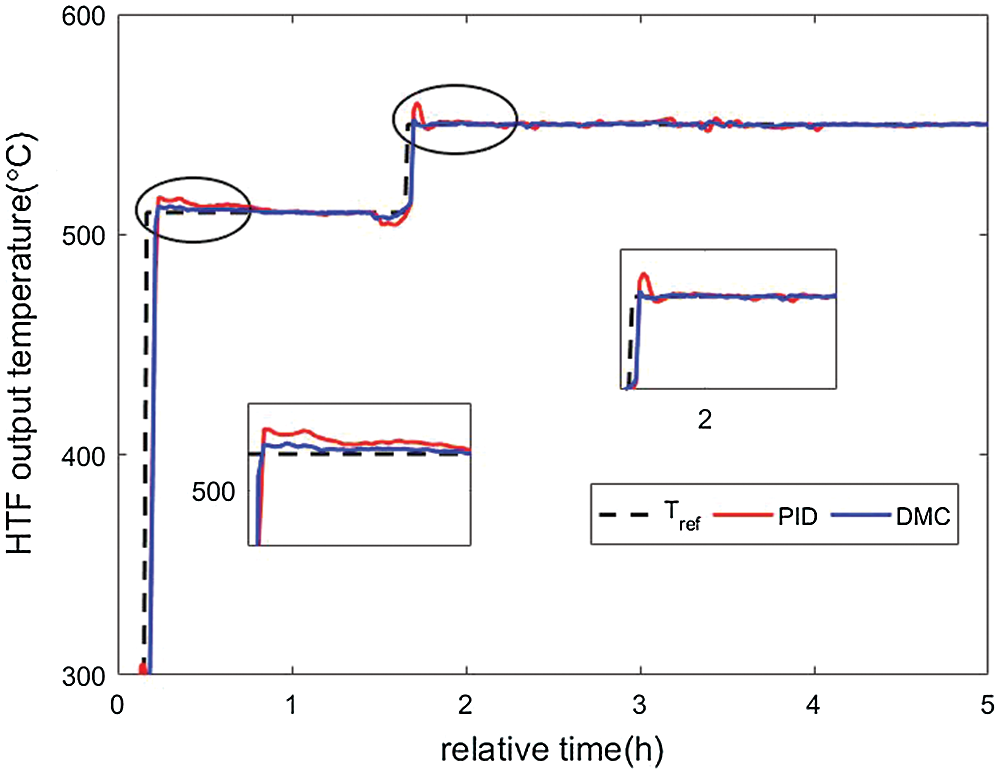
Figure 4: PID and DMC simulation comparison

Simulate a day with cloud cover and strong radiation intensity interference, the simulation data of the measurable disturbances I, Ta and Tfi used are shown in Fig. 5. Because there are several strong fluctuations in the irradiation intensity, the molten salt flow fluctuates greatly, which will bring big changes to the dynamic characteristics of the heat collection field, and make the model mismatch problem exist in the collector field model. The simulation result of the DMC controller is shown in Fig. 6. The performance of the controller deteriorates and there is a steady-state error. The simulation effect of the KFDMC controller is shown in Fig. 7. Due to the use of the Kalman filter to estimate the undetectable interference, the steady-state error is effectively eliminated, and the control effect is better. The curve of salt temperature at the outlet of the collector field in Fig. 7 is smoother and more stable than Fig. 6. In the 60th to 70th minutes of the simulation, the DNI fluctuates between 848.22 W/m2 and 874.06 W/m2, and the fluctuation is small. During this period, the maximum overshoot of the outlet salt temperature of the DMC control algorithm is 0.42%, and the maximum overshoot of the KFDMC control algorithm outlet salt temperature is 0.27%, and the maximum deviation of the outlet salt temperature of the KFDMC controller is 63.26% of the maximum deviation of the outlet salt temperature of the DMC algorithm. In the 100th to 110th minutes, DNI dropped sharply from 877.89 W/m2 to 520.47 W/m2, with large fluctuations. During this period, the maximum overshoot of the DMC algorithm was 7.14%, the maximum overshoot of the KFDMC controller was 3.39%, and the maximum deviation of the KFDMC controller outlet salt temperature was 47.5% of the maximum deviation of the DMC algorithm outlet salt temperature.

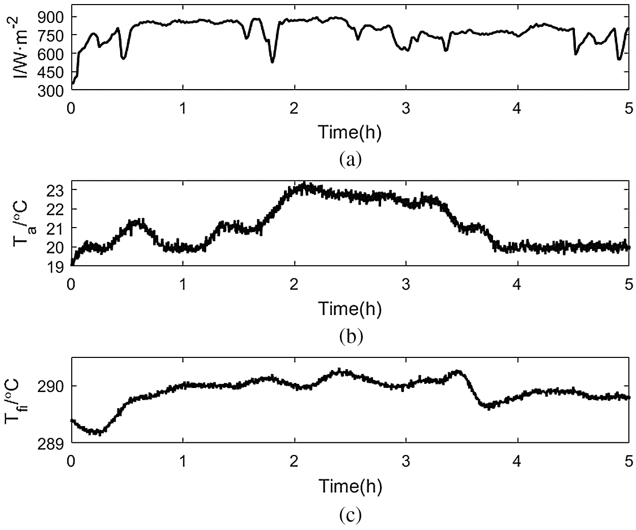
Figure 5: Perturbation data used in the heat field loop (a) Direct normal irradiation (b) Ambient temperature (c) Inlet molten salt temperature of collector field

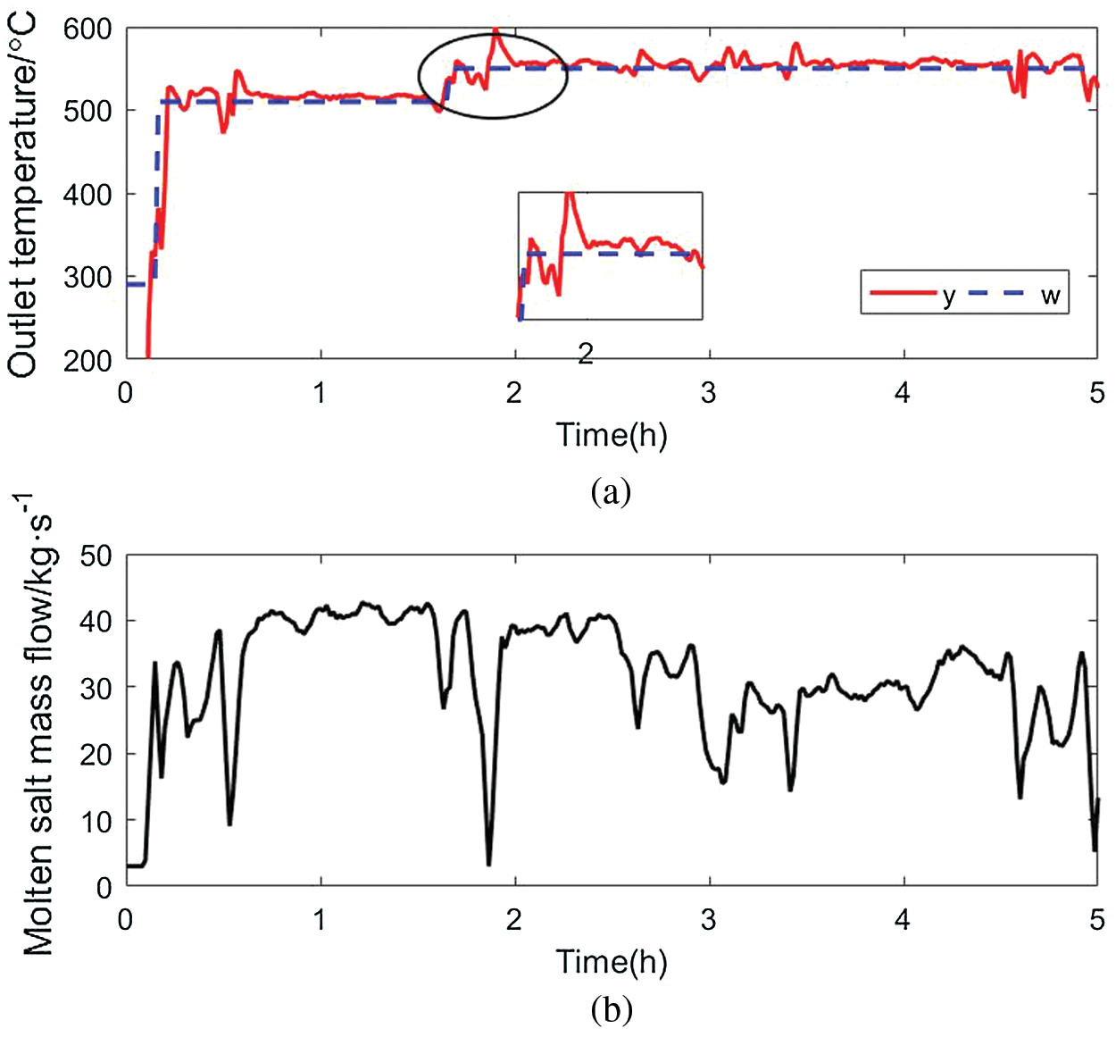
Figure 6: Dynamic matrix control results without filtering (a) Outlet molten salt temperature of collector field (b) Molten salt mass flow in collector field

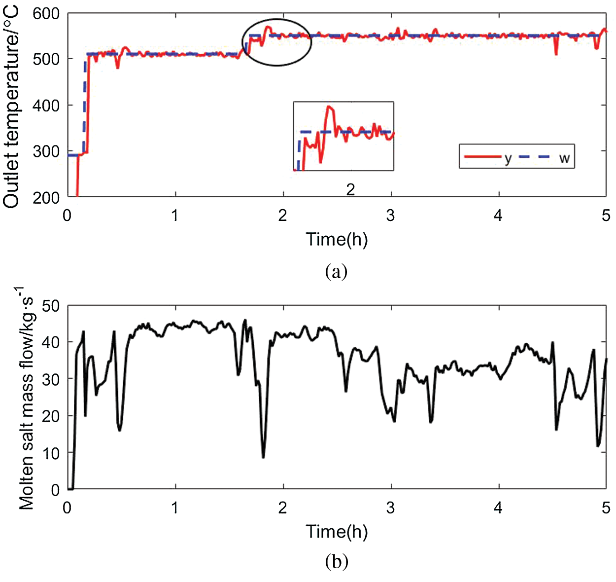
Figure 7: Dynamic matrix control with Kalman filter (a) Outlet molten salt temperature of collector field (b) Molten salt mass flow in collector field

The observation result of the Kalman filter is shown in Fig. 8, Fig. 8b is a simulation curve of 4 h~5 h. The result shows that the Kalman filter can estimate the state value more accurately, thus ensuring that the control performance is not affected. Where y is the outlet molten salt temperature of the collector field measured by the system, and yol is the open-loop predicted output estimated by steady state Kalman filter.

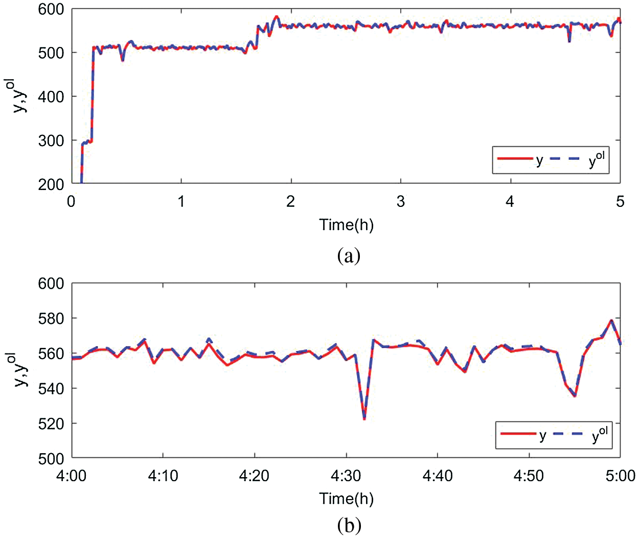
Figure 8: Kalman filter observations (a) Complete observation curve (b) Observation curve of the last hour

5  Conclusions

This paper proposes a DMC predictive controller with unmeasured interference estimation. By adding a steady-state Kalman filter in DMC, the LF heat collection system can effectively suppress the influence of measurement errors and unmodeled interference on the control effect. This article carries out simulation analysis for two different interference conditions. The results show that under the condition of clear weather and no cloud cover, the classic DMC predictive control algorithm has a good control effect, and its performance is better than PID controller. When there is cloud cover and the intensity of solar radiation fluctuates strongly throughout the day, considering measurement errors and model mismatch, the DMC predictive controller with unmeasured interference estimation has better control than the classic DMC predictive controller effect.

Funding Statement:This paper is supported by the National Natural Science Foundation of China (Grant No. 51667013) and the Science and Technology Project of State Grid Corporation of China (Grant No. 52272219000V).

Conflicts of Interest:The authors declare that they have no conflicts of interest to report regarding the present study.

References

 1.  Zhou, X. (2015). Experimental and theoretical investigation on the performance of a novel beam down system with fresnel heliostats and cavity receiver (Master Thesis). Shanghai Jiaotong University, China. [Google Scholar]

 2.  Huang, S. Y., Huang, S. H., Xu, G. L., Wang, X. M., Huang, X. M. et al. (2012). Principle and technology of solar thermal power generation. China: China Electric Power Press. [Google Scholar]

 3.  Alsharkawi, A., Rossiter, J. A. (2016). Gain scheduling dual mode MPC for a solar thermal power plant. IFAC-PapersOnLine, 49(18), 128–133. DOI 10.1016/j.ifacol.2016.10.151. [Google Scholar] [CrossRef]

 4.  Torrico, B. C., Roca, L., Normey-Rico, J. E., Guzan, J. L., Yebra, L. (2010). Robust nonlinear predictive control applied to a solar collector field in a solar desalination plant. IEEE Transactions on Control Systems Technology, 18(6), 1430–1439. [Google Scholar]

 5.  Galvez-Carrillo, M., Keyser, R. D., Ionescu, C. (2009). Nonlinear predictive control with dead-time compensator: Application to a solar power plant. Solar Energy, 83(5), 743–752. DOI 10.1016/j.solener.2008.11.005. [Google Scholar] [CrossRef]

 6.  Lima, D. M., Normeyrico, J. E., Santos, T. L. M. (2016). Temperature control in a solar collector field using Filtered Dynamic Matrix Control. ISA Transactions, 62(5), 39–49. DOI 10.1016/j.isatra.2015.09.016. [Google Scholar] [CrossRef]

 7.  Brus, L., Wigren, T., Zambrano, D. (2010). Feedforward model predictive control of a non-linear solar collector plant with varying delays. IET Control Theory & Applications, 4(8), 1421–1435. DOI 10.1049/iet-cta.2009.0315. [Google Scholar] [CrossRef]

 8.  Xu, H., Li, X., Xu, E. S. (2020). Research on temperature control of trough solar collector. Electric Power, 53(2), 83–91. [Google Scholar]

 9.  Lu, X. J., Dong, H. Y. (2017). Application of multi-model active fault-tolerant sliding mode predictive control in solar thermal power generation system. Acta Automatica Sinica, 43(7), 1241–1247. [Google Scholar]

10. Gallego, A. J., Camacho, E. F. (2012). Adaptative state-space model predictive control of a parabolic-trough field. Control Engineering Practice, 20(9), 904–911. DOI 10.1016/j.conengprac.2012.05.010. [Google Scholar] [CrossRef]

11. Zaversky, F., Medina, R., García-Barberena, J., Snchez, M., Astrain, D. (2013). Object-oriented modeling for the transient performance simulation of parabolic trough collectors using molten salt as heat transfer fluid. Solar Energy, 95(9), 192–215. DOI 10.1016/j.solener.2013.05.015. [Google Scholar] [CrossRef]

12. Sánchez, A. J., Gallego, A. J., Escao, J. M., Camacho, E. F. (2020). Parabolic trough collector defocusing analysis: Two control stages vs. four control stages. Solar Energy, 209(10), 30–41. DOI 10.1016/j.solener.2020.09.001. [Google Scholar] [CrossRef]

13. Luo, X. (2012). Disturbance observation method based on kalman filter applied in model predictive control (Master Thesis). Chongqing University, China. [Google Scholar]

14. Xie, Y. J., Ding, B. C., Chen, Q. (2017). Open-loop prediction method in dynamic matrix control based on Kalman filter. Control & Decision, 32(3), 419–426. [Google Scholar]

15. Li, S. Q., Ding, B. C. (2015). An overall solution to double-layered model predictive control based on dynamic matrix control. Acta Automatica Sinica, 41(11), 1857–1866. [Google Scholar]

16. Ding, B. C. (2016). Industrial predictive control. China: China Machine Press. [Google Scholar]

This work is licensed under a Creative Commons Attribution 4.0 International License, which permits unrestricted use, distribution, and reproduction in any medium, provided the original work is properly cited.