Energy Engineering

DOI: 10.32604/EE.2021.014759

ARTICLE

Robust Variable-Pitch Control Design of PMSG Via Perturbation Observer

Yilin Hu1, Yan Xie2, Bo Li3,*, Yiqiang Jiang1 and Fu Bao1

1Department of International Applied Technology, Yibin University, Yibin, 644000, China
2School of Information and Communication Engineering, Hainan University, Haikou, 570000, China
3School of Physics and Information Engineering, Zhaotong University, Zhaotong, 657000, China
*Corresponding Author: Bo Li. Email: 20192205026@stu.kust.edu.cn
Received: 27 October 2020; Accepted: 15 November 2020

1  Introduction

Energy is an essential material basis and support for human survival and social-economic development [1]. However, extensive consumption of limited fossil energy sources such as coal, oil, and natural [2] lead to severe environmental pollution, greenhouse effect, and increased global warming which are the common challenges in the world [3]. Hence, develop various renewable energy, e.g., wind [4], solar [5], geothermal [6], tides [7], waves [8], etc., and improve its efficiency have become a global consensus [9]. Specially, wind energy is one of promising alternative energy with the merits of pollution-free, cheap, widespread, and unlimited supply [10]. According to statistics of Renewables 2020 Global Status Report, the total growth rate of wind power capacity is around 228.79% in the globe over the past decade, which leads to a total of 651 GW installation up to 2019 [11].

Currently, permanent magnet synchronous generator (PMSG) is an attractive choice of wind turbine (WT) due to its large thrust, low loss, high-efficiency density, and high energy conversion efficiency [12]. And the operating regions of PMSG can be divided into three parts, as shown in Fig. 1. Specially, in Region 2, wind speed is between cut-in wind speed and rated value. The task of WT is to control turbine speed at the optimal value for extracting the maximum output power [13]. In Region 3, wind speed is between rated value and cut-out wind speed. The variable pitch controller adjusts the blade pitch angle to maintain output power at its rated value as the capacities of generator and converter are limited [14].

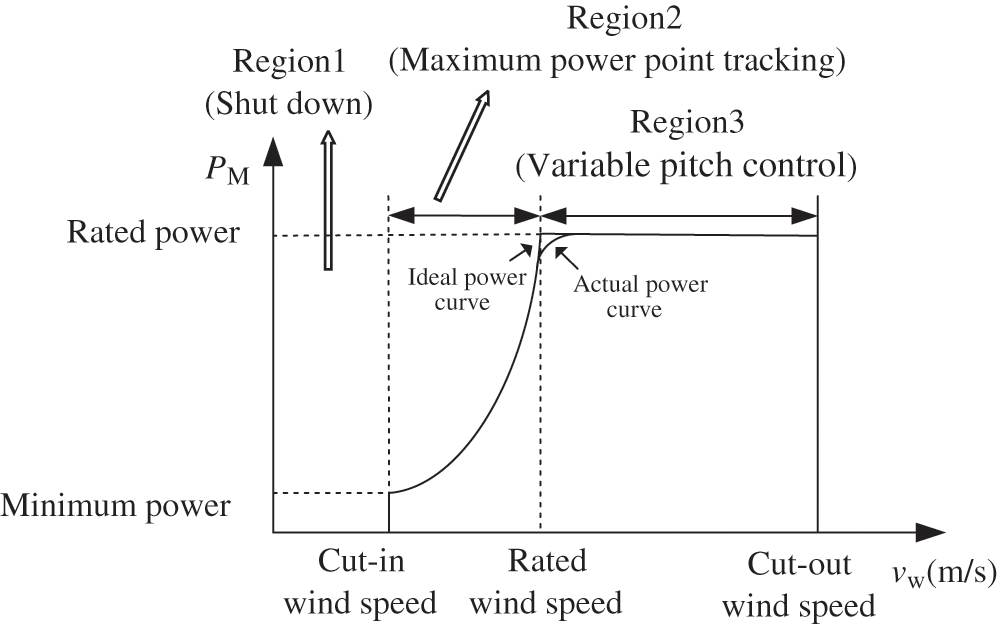
Figure 1: Three operating regions of PMSG

Various variable pitch control techniques have been reported in publications during the past decades so far. Conventional vector control (VC) using proportional-integral (PI) and proportional-integral-derivative (PID) control are widely adopted in industrial processes owing to its strengths of simple configuration and convenient implementation [15]. Nevertheless, it is an approximated linearization model based on an equilibrium point in which performance will inevitably degrade when the operating point is changed [16]. The linear quadratic Gaussian (LQG) is another common method in pitch angle control which can provide high robustness in terms of the phase and gain margins [17]. Nevertheless, wind energy conversion systems (WECS) are highly nonlinear due to the randomicity, intermittence, and seasons of wind energy such that this linear controller only has poor performance [18]. Hence, a series of advanced control strategies for pitch angle control, e.g., nonlinear control, fuzzy control, robust control, and self-adaptive control are presented to overcome the defects of VC and LQG. Adaptive PID [19] control and fuzzy self-tuning PID control [20] tune PID parameters on-line, which can suppress a variety of non-linear, time-varying factors. But the inherent drawback of PID is still retained in the above frameworks, which cannot obtain consistent control performance [21]. Moreover, Senjyu et al. [22] proposes a generalized predictive control (GPC) for wind generators in all operating regions which can effectively mitigate the adverse effects of changed operating points. Van et al. [23] develops a low-cost fuzzy logic controller for variable-speed WT without consideration of expensive wind speed measurements. And Wang et al. [24] designs a two-degree-of-freedom motion mechanism with feedback linearization control (FLC) for the large WT with improved robustness and stability. Moreover, multi-layer perceptron and radial basis function neural networks are investigated in work [25] to prevent WT from overloading or shutting down during high wind speed. Recently, perturbation observer has been applied widely in nonlinear system control, such as WECS [26], photovoltaic systems [27], VSC-HVDC systems [28] and so on, which can on-line estimate unknown nonlinearities, parametric uncertainties, and time-varying external disturbances for nonlinear system without the requirement of detailed system model [29].

In this work, a perturbation observer based sliding-mode control (POSMC) is adopted for PMSG to limit the turbine output power and generator speed in Region 3. Firstly, the perturbation observer generates the new perturbation via combining the system nonlinearities, parametric uncertainties, unmodelled dynamics, and time-varying external disturbances. Then sliding mode control is utilized to completely compensate the perturbation estimation in real-time. The proposed POSMC retains the strong robustness of sliding-mode control (SMC), and only require the measurements of d-q axis current and mechanical rotation speed. Three case studies are studied by Matlab/Simulink, e.g., ramp wind speed, random wind speed, and parameter uncertainty. Simulation results validate that, compared with VC control, feedback linearization control (FLC) and nonlinear adaptive control (NAC), POSMC can achieve satisfactory robust control performance under various operating conditions.

The rest of this article is organized as follows: Section 2 gives the model of PMSG system; Section 3 introduces the theory of POSMC; Section 4 develops the detailed design of POSMC for variable-pitch PMSG. In Section 5, case studies results are discussed and analyzed. And the last Section summarizes this work and draws conclusions.

2  Modelling of PMSG System

A representative topology of PMSG system is described in Fig. 2. Firstly, mechanical power is transformed into electrical power via WT. Then, the electrical power is injected into power grid through back-to-back voltage source converters, filters, and the transformer. Specially, the major task of the machine-side converter (MSC) is to capture mechanical power and provide the required stator voltage, while active power and reactive power are regulated by the grid-side converter (GSC) [30]. In addition, MSC and GSC can realize a fully decoupled control by the DC link.

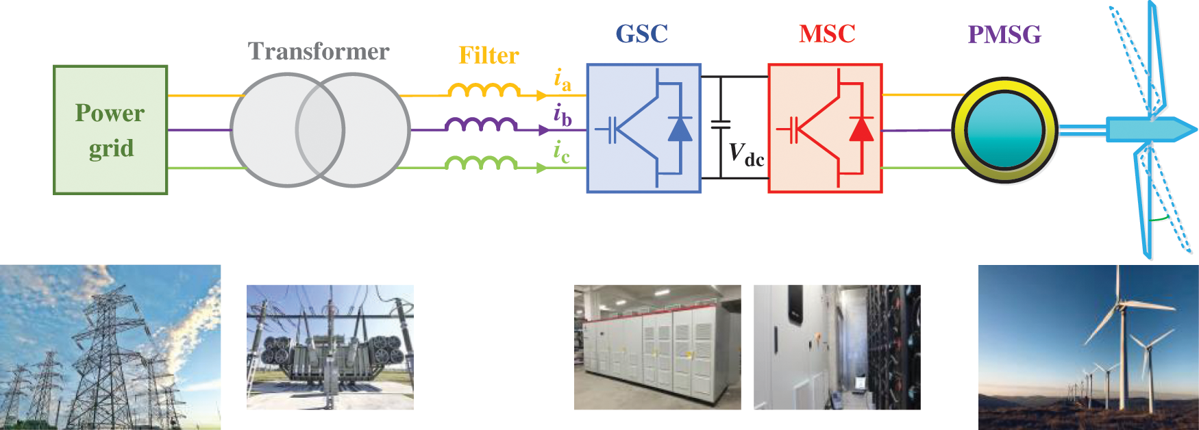
Figure 2: A representative topology of PMSG system

2.1 WT Model

The tip speed ratio λ of WT is denoted as [15]

λ=RωmV (1)

where R represents the blade radius, ωm is the mechanical rotation speed, V is the wind speed.

According to aerodynamic theory, the electrical power extracted by the WT can be described as

Pm=12ρπR2V3CP(β,λ) (2)

where ρ is the air density. And the power coefficient CP(β,λ) can be represented by pitch angle β and λ

Cp=0.22(116λi−0.4β−5)e−12.5λi (3)

1λi=1λ+0.08β−0.035β3+1 (4)

2.2 Generator System Model

The voltage and torque equations of PMSG can be denoted as

Vd=idRs+Lddiddt−ωeLqiq (5)

Vq=iqRs+Lqdiqdt+ωe(Ldid+Ke) (6)

Te=p[(Ld−Lq)idiq+iqKe] (7)

where Vd and Vq represent d-q axis stator voltages, id and iq are d-q axis stator currents, Ld and Lq are d-q axis inductances, ωe=pωm is electrical rotate-speed, Te is the electromagnetic torque, p is the number of pole pairs, and Ke is the permanent magnetic flux.

2.3 Drive Train Model

The dynamics model of mechanical shaft system can be represented by

Jtotdωmdt=Tm−Te (8)

Tm=12ρπR5Cp(λ,β)λ3ωm2 (9)

where Jtot denote the total inertia of the drive train, Tm is the mechanical torque, D is the viscous damping coefficient. Note that Te has a much faster response than Tm, thus let T˙e=0 in this paper to realize simplified calculation.

2.4 Pitch Angel Control Model

Pitch angel control actuator could regulate the blade pitch based on the required value. And the first-order linear model of pitch angel control actuator without considering the delay characteristics can be given as [14]

β˙=−βτβ+βrτβ (10)

where βr is the required pitch angle, and τβ is the time constant of actuator.

3  Perturbation Observer Based Sliding-Mode Control

3.1 Design of SMSPO

An uncertain nonlinear system is denoted as

{x˙=Ax+B(a(x)+b(x)u+d(t))y=x1 (11)

where x=[x1,x2,…,xn]T∈Rn , u∈R , y∈R denote state vector, control input, and system output, respectively. a(x):Rn↦R and b(x):Rn↦R represent unknown smooth functions, and d(t):R+↦R is time-varying external disturbance.

The perturbation of system (11) is described as

ψ(x,u,t)=a(x)+(b(x)−b0)u+d(t) (12)

where b0 is constant control gain.

Based on Eq. (12), the last state xn of system (11) is represented as

x˙n=a(x)+(b(x)−b0)u+d(t)+b0u=ψ(x,u,t)+b0u (13)

Define a fictitious state xn+1 to denote perturbation ψ(x,u,t) , then the original nth order system can be extended into the (n+1)th order augmented system, yields

{y=x1x˙1=x2⋮x˙n=xn+1+b0ux˙n+1=ψ(⋅) (14)

Define the extended state vector xextend=[x1,x2,…,xn,xn+1]T , and propose the assumptions:

Assumption 1: b0 is selected to meet |b(x)/b0−1|≤θ<1 , where θ represents a positive constant.

Assumption 2: perturbation ψ(x,u,t) and its derivative ψ˙(x,u,t) are bonded within the domain: |ψ(x,u,t)|≤γ1 , |ψ˙(x,u,t)|≤γ2 with ψ(0,0,0) = 0 and ψ˙(0,0,0) = 0, where γ1 and γ2 are positive constants.

Suppose y = x1 is the sole measurable state, a (n+1)th order SMSPO is designed to estimate the system states and perturbation, obtains

{x^˙1=x^2+α1x~1+k1sat(x~1)⋮x^˙n=ψ^(⋅)+αnx~1+knsat(x~1)+b0uψ^˙(⋅)=αn+1x~1+kn+1sat(x~1) (15)

where x^ represents the estimated value of x, x~=x−x^ denotes the estimation error, positive constants αi (i = 1,2,…,n) are observer gains, and positive constants ki (i = 1,2,…,n) are sliding surface gains.

3.2 Design of Sliding-Mode Controller

An estimated sliding surface is defined as

S^(x,t)=∑i=1n⁡ρi(x^i−yd(i−1)) (16)

where the estimated sliding surface gains ρi=Cn−1i−1λcn−i (i = 1,2,…,n) place all the poles of estimated sliding surface on the left half −λc of complex plane with λc>0 .

Finally, POSMC of system is given as

u=1b0[yd(n)−∑i=1n−1⁡ρi(x^i+1−yd(i))−ςS^−φsat(S^,òc)−ψ^(⋅)] (17)

where ς and φ are controller gains, òc is the thickness layer boundary of controller.

4  POSMC Design of Variable-Pitch PMSG

4.1 State-Space Equation of PMSG

The state-space equation of PMSG is represented by

x˙=f(x)+g1(x)u1+g2(x)u2+g3(x)u3 (18)

where

f(x)=[−βτβ−RsLdid+ωeLqLdiq−RsLqiq−1Lqωe(Ldid+Ke)1JtotTm] (19)

g(x)=[−βτβ00001Ld00001Lq00000] (20)

x=[βidiqωm]T (21)

u=[u1,u2,u3]T=[βr,Vd,Vq]T (22)

y=[y1,y2,y3]T=[h1(x),h2(x),h3(x)]T=[ωm,id,iq]T (23)

where x∈R4 , u∈R3 , and y∈R3 are state vector, control input, and system output, respectively. Rs is the stator resistance, Vd and Vq are d-q axis stator voltages, and ωe=pωm is the electrical generator rotation speed.

4.2 Pitch Angle Control

Differentiate control output y1=ωm until it appears explicitly, as

y¨1=1JtotT˙m=A(−Cpωm−RVF2E)dωmdt−AEβτβ[−0.088e−12.5τE−0.08V2F2+0.105β2(1+β3)2]+AEτβ[−0.088e−12.5τE−0.08V2F2+0.105β2(1+β3)2]u1 (24)

where

A=ρπR2V32ωm (25)

E=(39.27−319τ+1.1β)e−12.5τ (26)

F=ωmR+0.08βV (27)

τ=1λ+0.08β−0.035β3+1 (28)

Eq. (24) can be rewritten into matrix form, yields

y¨1=F1(x)+B1(x)u1 (29)

where

F1(x)=A(−Cpωm−RVF2E)dωmdt−AEβτβ[−0.088e−12.5τE−0.08V2F2+0.105β2(1+β3)2] (30)

B1(x)=AEτβ[−0.088e−12.5τE−0.08V2F2+0.105β2(1+β3)2] (31)

Note that det[B1(x)]≠0 when V≠0 and β≠0 , thus B1(x) is nonsingular in all the feasible zone. In other words, above input-output linearization is valid.

Define perturbation ψ1(⋅) to describe the nonlinearities and uncertainties of F1(x) and B1(x) , yields

ψ1(⋅)=F1(x)+(B1(x)−B1(0))u1 (32)

where B1(0)=b10 is constant control gain.

Define tracking error e1=[ωm−ωm∗] where ωm∗ is the reference of ωm , one can obtain

e¨1=ψ1(⋅)+B1(0)u1−ω¨m∗ (33)

Then, a third order sliding-mode state and perturbation observer (SMSPO) is adopted to estimate ψ1(⋅) , as

{ω^˙m=ω˙^m+α11ω~m+k11sat(ω~m,òo)ω˙^˙m=ψ^1(⋅)+α12ω~m+k12sat(ω~m,òo)+B1(0)u1ψ^˙1(⋅)=α13ω~m+k13sat(ω~m,òo) (34)

where positive constants α11 , α12 , α13 , k11 , k12 , and k13 are observer gains.

The estimated sliding surface of system (29) is chosen as

S^1=ρ1(ω^m−ωm∗)+ρ2(ω˙^m−ω˙m∗) (35)

Finally, the POSMC of system (29) is designed as

u1=1B1(0)[ω¨m∗−ρ1(ω˙^m−ω˙m∗)−ς1S^1−φ1sat(S^1,òc)−ψ^1(⋅)] (36)

where ρ1 is estimated sliding surface gains, ς1 and φ1 are controller gains.

4.3 Generator Control

Differentiate control output y=[y2,y3]T=[id,iq]T until it appears explicitly, as

[y˙2y˙3]=[F2(x)F3(x)]+B2(x)[u2u3] (37)

where

F2(x)=1Ld(−idRs+ωeLqiq) (38)

F3(x)=−RsLqiq+1Lqωe(Ldid+ke) (39)

B2(x)=[B21B22B23B24]=[1Ld001Lq] (40)

Note that det[B2(x)]=1LdLq≠0 , thus B2(x) is nonsingular in all the feasible zone. In other words, above input-output linearization is valid.

Define perturbation ψ2(⋅) and ψ3(⋅) to describe the nonlinearities and uncertainties of F2(x) , F3(x) , and B2(x) , yields

[ψ2(⋅)ψ3(⋅)]=[F2(x)F3(x)]+(B2(x)−B2(0))[u2(x)u3(x)] (41)

where B2(0)=[b2000b30] is constant control gain.

Define tracking error e=[e2e3]T=[id−id∗,iq−iq∗] , one can obtain

[e˙2e˙3]=[ψ2(⋅)ψ3(⋅)]+B2(0)[u2u3] (42)

Then, two second order sliding-mode perturbation observers (SMPOs) are adopted to estimate ψ2(⋅) and ψ3(⋅) , as

{i^˙d=ψ^2(⋅)+α21i~d+k21sat(i~d,òo2)+b20u2ψ^˙2(⋅)=α22i~d+k22sat(i~d,òo2) (43)

{i^˙q=ψ^3(⋅)+α31i~q+k31sat(i~q,òo2)+b30u3ψ^˙3(⋅)=α32i~q+k32sat(i~q,òo2) (44)

where positive constants α21 , α22 , α31 , α32 , k21 , k22 , k31 and k32 are observer gains.

The estimated sliding surface of system (37) is chosen as

[S^2S^3]=[i^d−id∗i^q−iq∗] (45)

Finally, the POSMC of system (37) is designed as

[u2u3]=1B2(0)[i˙d∗−ς2S^2−φ2sat(S^2,òc2)−ψ^2(⋅)i˙q∗−ς3S^3−φ3sat(S^3,òc2)−ψ^3(⋅)] (46)

where ς1 , ς2 , φ1 , and φ2 are controller gains.

At this end, the overall block diagram of POSMC is shown in Fig. 3.

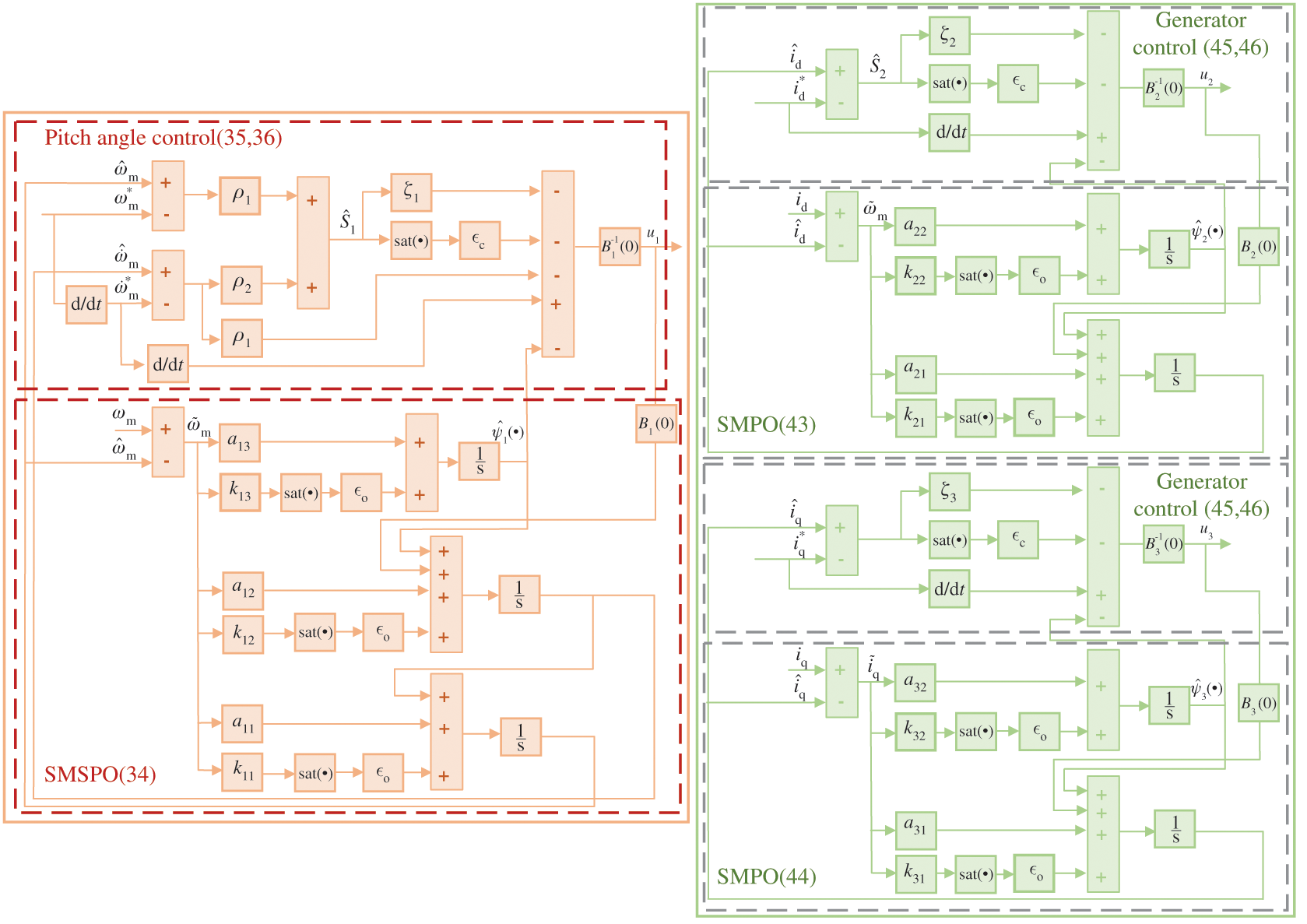
Figure 3: The overall block diagram of POSMC

4.4 Analysis and Discussion

As described in Assumption 2, the perturbation and its derivative are locally bounded. And the deduction of these bounds is given as

ψ1(⋅)=F1(x)+(B1(x)−B1(0)B1(x))[−ρ1(ω˙^m−ω˙m∗)−ς1S^1−φ1sat(S^1,òc)+ω¨m∗−ψ^1(⋅)]=F1(x)+(B1(x)−B1(0)B1(x))[−ρ1e11−ς1S^1−φ1sat(S^1,òc)+ε11] (47)

ψ2(⋅)=F2(x)+(B21(x)−B21(0)B21(x))(−ς2S^2−φ2sat(S^2,òc2)+i˙d∗−ψ^2(⋅))=F2(x)+(B21(x)−B21(0)B21(x))(−ς2S^2−φ2sat(S^2,òc2)+ε21) (48)

ψ3(⋅)=F3(x)+(B24(x)−B24(0)B24(x))(−ς3S^3−φ3sat(S^3,òc2)+i˙q∗−ψ^3(⋅))=F3(x)+(B24(x)−B24(0)B24(x))(−ς3S^3−φ3sat(S^3,òc2)+ε22) (49)

ψ˙1(⋅)=F˙1(x)+(B1(x)−B1(0)B1(0))(−ρ1e˙11−ς1S^1˙−φ1sat(S^1˙,òc)+ε˙11) (50)

ψ˙2(⋅)==F˙2(x)+(B21(x)−B21(0)B21(0))(−ς2S^2˙−φ2sat(S^2˙,òc2)+ε˙21) (51)

ψ˙3(⋅)==F˙3(x)+(B24(x)−B24(0)B24(0))(−ς3S^3˙−φ3sat(S^3˙,òc2)+ε˙22) (52)

|ψ1|≤11−θ1|F1(x)|+θ11+θ1(‖ρ1‖‖e11‖+‖ς1‖+‖φ1‖+|ϵ11|) (53)

|ψ2|≤11−θ2|F2(x)|+θ21+θ2(‖ς2‖+‖φ2‖+|ϵ21|) (54)

|ψ3|≤11−θ3|F3(x)|+θ31+θ3(‖ς3‖+‖φ3‖+|ϵ22|) (55)

|ψ˙1|≤|F˙1(x)|+|B1(x)||u1|+θ1(‖ρ1‖‖e˙11‖+‖ς1‖+‖φ1‖+|ϵ˙11|) (56)

|ψ˙2|≤|F˙2(x)|+|B21(x)||u2|+θ2(‖ς2‖+‖φ2‖+|ϵ˙21|) (57)

|ψ˙3|≤|F˙3(x)|+|B24(x)||u3|+θ3(‖ς3‖+‖φ3‖+|ϵ˙22|) (58)

Hence, the validity of the developed perturbation observer is demonstrated.

5  Case Studies

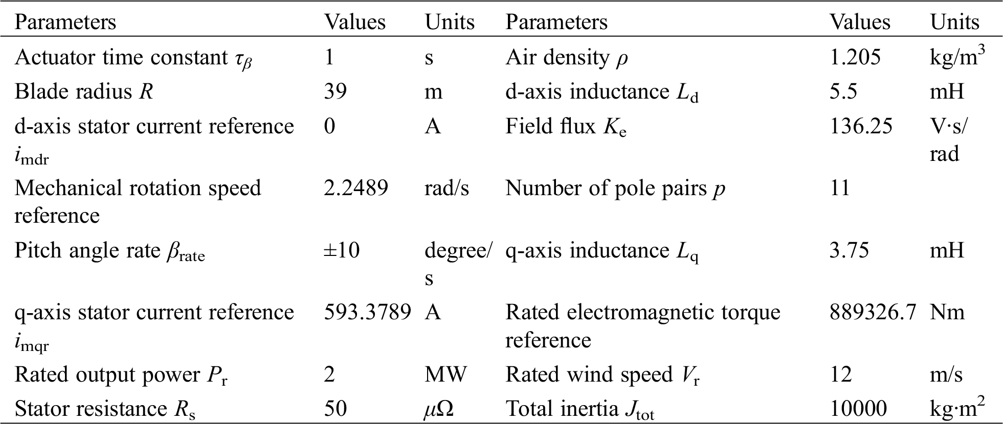
Three cases, e.g., ramp wind speed, random wind speed, and parameter uncertainty, are undertaken to assess the performance of POSMC compared with that of VC [15], FLC [24], and NAC [14]. The simulation is implemented based on MATLAB R2019a by a desktop computer with an Intel® Core™ i5 CPU at 3.4 GHz and 16 GB of RAM. And the parameters of PMSG and POSMC are listed in Tabs. 1 and 2, respectively.

Table 1: Parameters of PMSG

Table 2: Parameters of POSMC

5.1 Ramp Wind Speed

A ramp wind signal changing from 18 m/s to 14 m/s is exerted to WECS, as shown in Fig. 4. The simulation outcomes of four controllers under ramp wind are shown in Fig. 5. One can easily find that VC has the longest convergence time and the biggest tracking error of ωm due to its control gains are obtained by local linearization of specific system operating point. FLC has obvious oscillation of ωm , Pm, and Qm during running period which needs full state measurements. Meanwhile, NAC has the highest overshoot of imd and imq compared with other three methods. And POSMC can obtain the satisfactory control performance with the fast convergence speed and the small tracking error. Specially, the convergence time of VC, FLC, NAC, and POSMC in terms of ωm are 4.16 s, 5.71 s, 5.80 s, and 16.46 s, respectively. And the maximum overshoot of Pm of VC, FLC, NAC and POSMC is 8.70% and 3.55%, 1.25% and 0.15%, respectively. Meanwhile, the errors between the estimations and actual values of the designed observers are shown in Fig. 6 which provides satisfactory estimation.

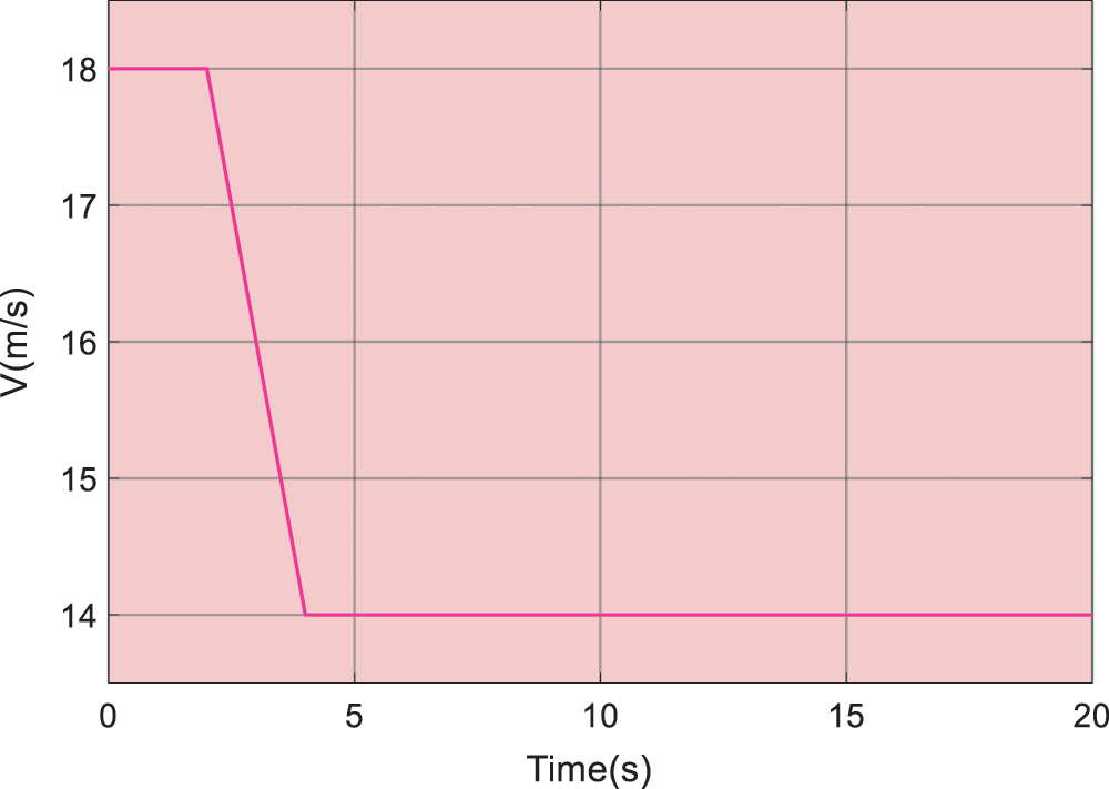
Figure 4: Ramp wind curve

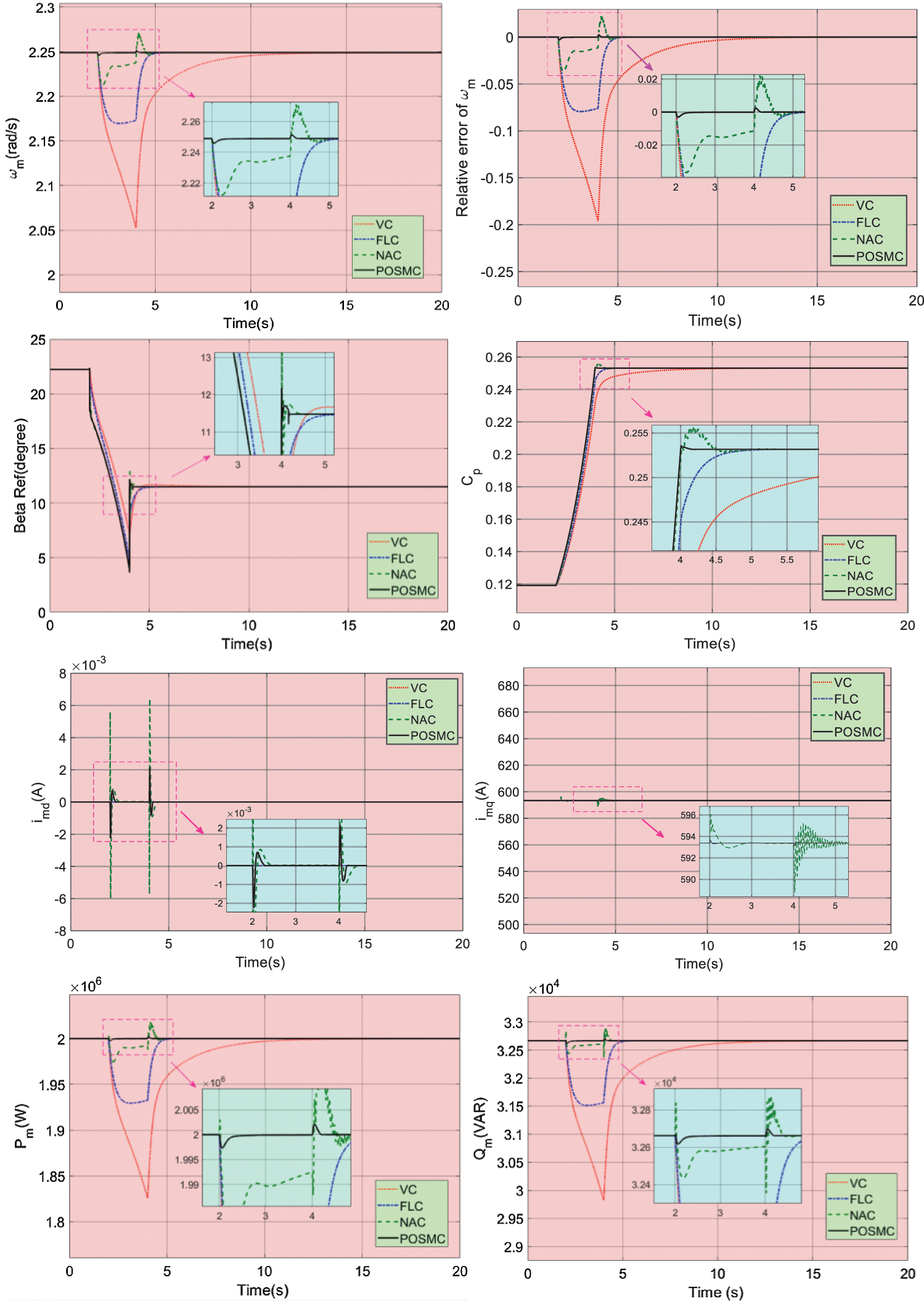
Figure 5: The simulation outcomes of four controllers under ramp wind speed

Figure 6: The error between the estimations and actual values of the designed observers under ramp wind speed

5.2 Random Wind Speed

The random wind curve is denoted in Fig. 7. And Fig. 8 describes the simulation outcomes under such scenario. Obviously, POSMC keeps ωm , Pm and Qm around their rated value during all the simulation time with the smallest overshoot and consistent control performance. Meanwhile, VC, FLC, and POSMC have the nearly similar control performace of imd and imq. And Fig. 9 denotes the error between the estimations and actual values of the designed observers which prove that the developed SMSPO and SMPO have excellent tracking effects.

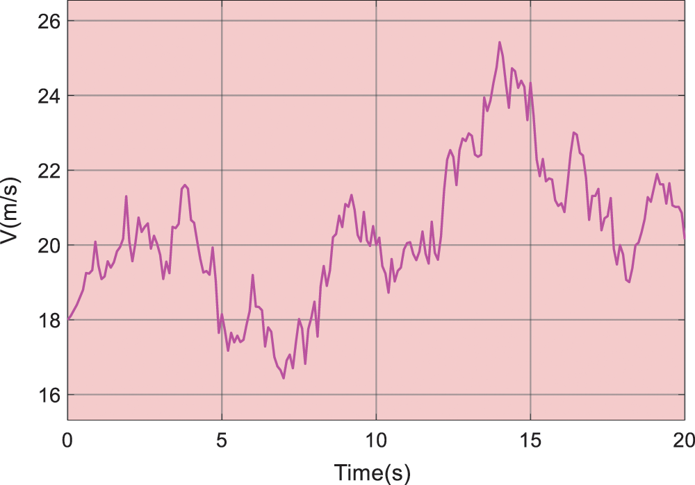
Figure 7: Random wind curve

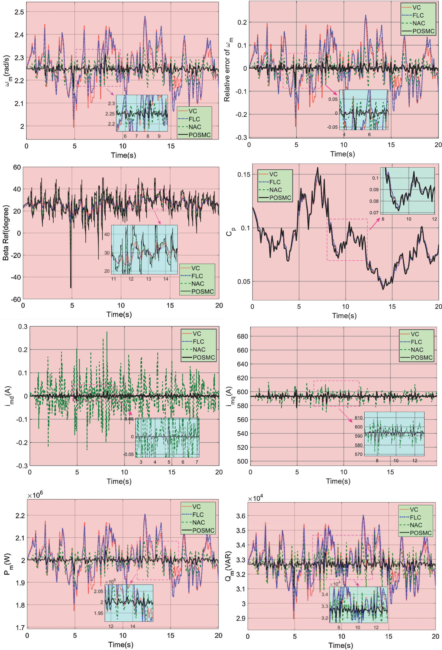
Figure 8: The simulation results of four controllers under random wind speed

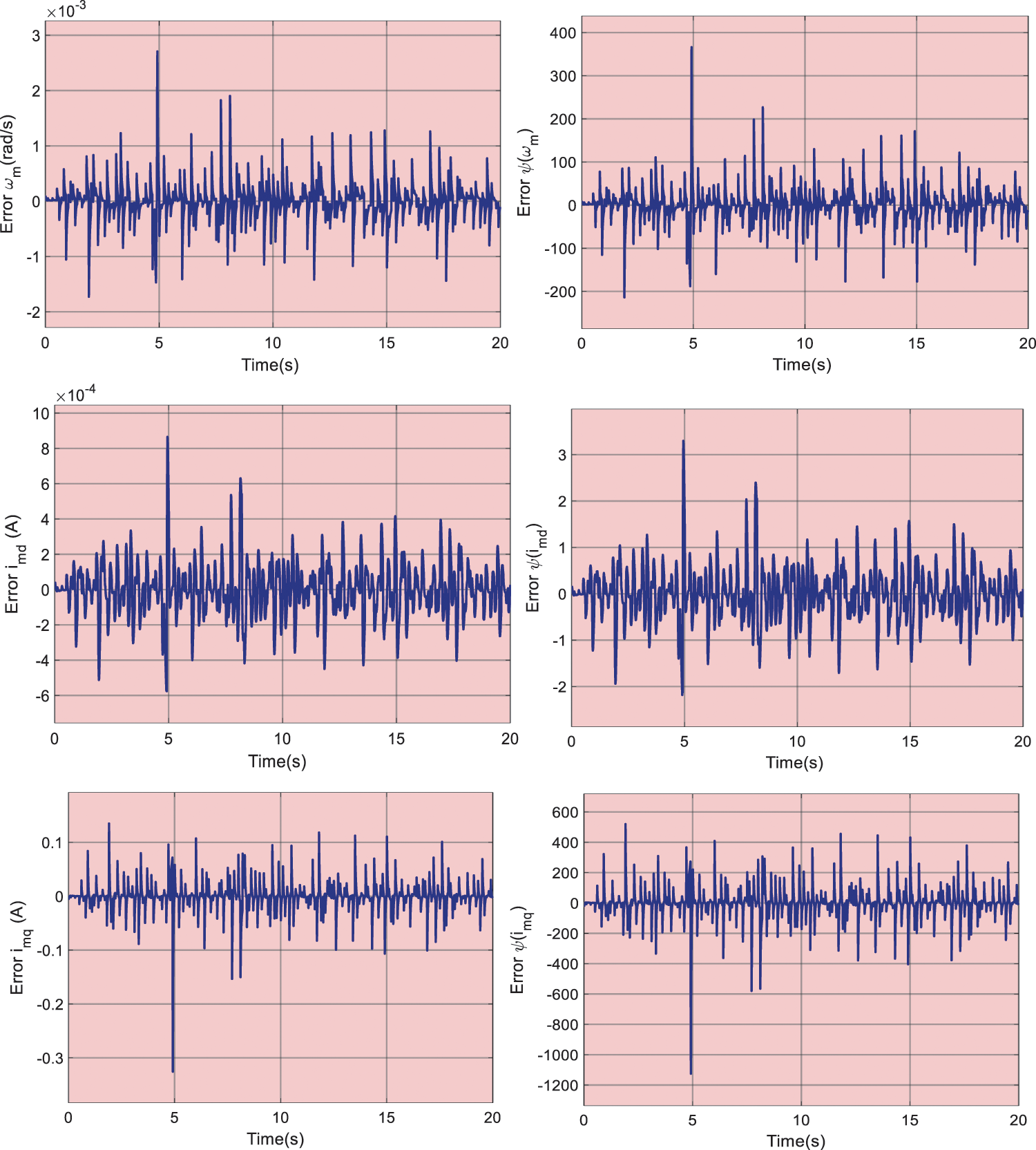
Figure 9: The error between the estimations and actual values of the designed observers under random wind speed

5.3 Parameter Uncertainty

In this case, the variation of field flux Ke from 1 (p.u.) at t = 4s to 0.9 (p.u.) at t = 9s is implemented to system for evaluating the robustness of four controllers. And wind speed remains at 18 m/s during all the simulation time. Fig. 10 shows the simulation outcomes of four controllers under above scenario. It is clear that POSMC can restore perturbed system with the fastest speed. Though VC and FLC have the lower oscillation of imd because of the simple mechanism, they have the worst control performance in other seven output variables. And the maximum overshoot of ωm of VC, FLC and NAC is 5.16% and 1.24% and 0.36%, respectively. While POSMC can realize nearly smooth tracking performance of all output variables with the strongest robustness.

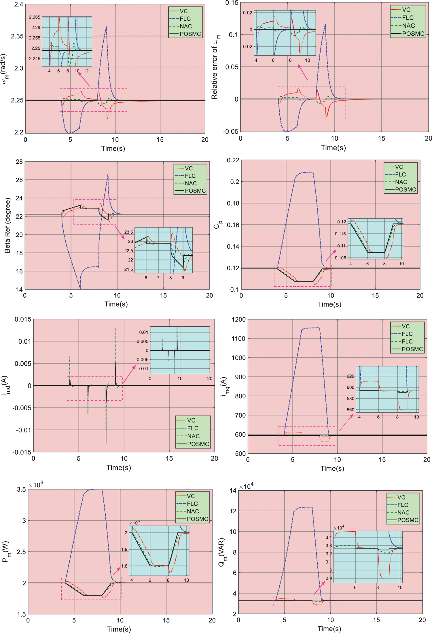
Figure 10: The simulation outcomes of four controllers under parameter uncertainty

5.4 Statistical Analysis

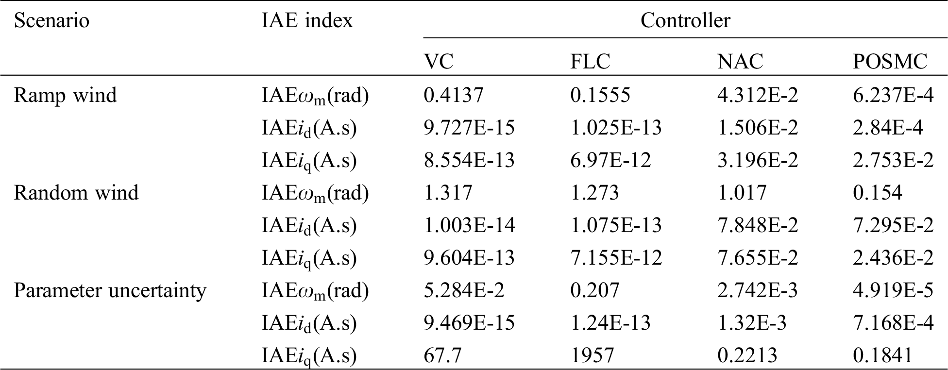
Integral absolute error index IAEx=∫0T|x−x∗|dt is widely used in the quantitative analysis of control errors, which describes the error accumulation of system output compared to its reference value over a period of time T. Tab. 3 gives IAE ωm , IAE id , and IAE iq of four controllers in three cases. VC obtains the smallest IAE id and IAE iq in most cases thanks to its simple structure, but it has the longest recovery time and most obvious oscillations of ωm due to the linear frame. And POSMC can obtain the smallest IAE ωm in all the four controllers under three cases. Moreover, the overall control costs ∫0T(|βr|+|Vd|+|Vq|)dt of four controllers are shown in Fig. 11. Although VC have the lower control costs than POSMC in ramp wind, it has poor control performance. While POSMC has the smallest control costs than VC, FLC, and NAC in random wind due to the integration of nonlinear real-time perturbation estimation and robust SMC structure. Specially, the overall control costs of POSMC are 99.58%, 99.52% and 96.73% of that of VC, FLC, and NAC in random wind.

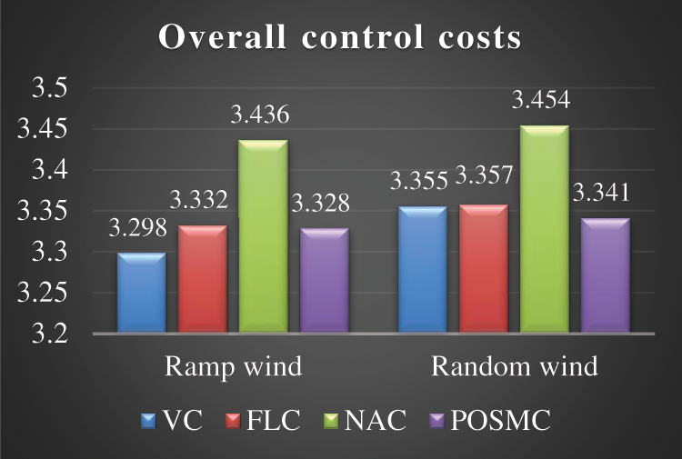
Figure 11: The overall control costs of four control approaches

Table 3: IAE indexes of four control approaches obtained in three scenarios (p.u.)

6  Conclusions

In this paper, POSMC is applied in variable-pitch control of PMSG to limit generator’s output power at its rated value when the wind speed is higher than rated value. The main novelties/contributions can be concluded as follows:

     i)  POSMC combines nonlinearities, parametric uncertainties, unmodelled dynamics, and time-varying external disturbances into a new perturbation estimating via the perturbation observer. Subsequently, sliding mode control is designed to completely make up for the perturbation estimation in real-time for the sake of realizing a global consistent control performance and improving the robustness of the system under various operation conditions.

    ii)  Compared with VC, POSMC is designed based on nonlinear architecture which is not affected by the changed system operating points.

   iii)  Compared with FLC, POSMC only requires the measurements of d-q axis current and mechanical rotation speed ωm rather than full-state measurements which are easy to implement.

    iv)  Compared with NAC, POSMC has the better control performance in ramp wind and random wind, the higher robustness in terms of parameter uncertainty, the smaller IAE indexes and overall control costs. Specially, the IAE ωm of POSMC is only 1.45%, 15.14% and 1.79% of that of NAC in ramp wind, random wind and parameter uncertainty, respectively. And the overall control costs of POSMC are 96.86% and 96.73% of that of NAC in ramp wind and random wind, respectively.

Future studies will be focused on carrying out the HIL experiment of variable-pitch PMSG to further prove the implementation feasibility of POSMC.

Funding Statement: The authors thankfully acknowledge the support of the Noise problem of electric vehicle brushless DC motor starting (S202010641109).

Conflicts of Interest: The authors declare that they have no conflicts of interest to report regarding the present study.

This work is licensed under a Creative Commons Attribution 4.0 International License, which permits unrestricted use, distribution, and reproduction in any medium, provided the original work is properly cited.