| Energy Engineering |
DOI: 10.32604/EE.2021.014949
ARTICLE
Wind Power Revenue Potential: Simulation for Finland
Department of Mechanical Engineering, Aalto University, Espoo, Finland
*Corresponding Author: Sakarias Paaso. Email: sakarias.paaso@aalto.fi
Received: 10 November 2020; Accepted: 18 March 2021
Abstract: Potential revenue from wind power generation is an important factor to be considered when planning a wind power investment. In the future, that may become even more important because it is known that wind power generation tends to push electricity wholesale prices lower. Consequently, it is possible that if a region has plenty of installed wind power capacity, revenue per generated unit of electricity is lower there than could be assumed by looking at the mean electricity wholesale price. In this paper, we compare 17 different locations in Finland in terms of revenue from wind power generation. That is done by simulating hourly generation with three different turbine types at two different hub heights and multiplying that by the hourly electricity spot price for years 2018 and 2019. Estimated revenues differ greatly between locations and turbine types, major factor being technical potential i.e., the amount of electricity generated. Differences between revenues per generated MWh seem to be small, however, the smallest figures being on the western coast where installed capacities are also the largest in Finland.
Keywords: Wind power; renewable energy; resource assessment; revenue; Finland
Climate change is an internationally recognized, global problem that is caused by excessive stock of greenhouse gases in the atmosphere. One way of responding to it is decreasing greenhouse gas emissions emitted into the atmosphere, which slows down the rate of change. A major greenhouse gas is carbon dioxide (CO2) that is mainly emitted when burning fossil fuels as a source of energy to be used for example in transportation and electricity generation. However, there are energy sources that can be utilized with minimal emissions. A group belonging to those is renewable energy sources that covers for example biomass, hydro, solar and wind power. Wind power is a rapidly growing source of energy in electricity production in Finland. In only ten years, between 2009 and 2019, cumulative installed wind power capacity grew from around 200 MW to 2300 MW [1]. In the same period, annual power production increased from couple hundred to around 6000 GWh and in 2019, wind power accounted for 9% of total electricity generation in Finland which is 66 TWh [1,2]. According to data provided by Etha Wind [3], around 18500 MW of new capacity is either under construction or in different planning phases with planned start of production ranging from 2020 to 2030.
Nordic electricity wholesale market, Nord Pool, covers four countries: Denmark, Norway, Sweden and Finland. Its day-ahead pricing mechanism is relatively simple: For each hour electricity sellers and buyers bid the volume (MWh/h) they are willing to produce or buy and at which price. Demand and supply curves are then formed from these individual bids and the price sets at the level where the curves cross. The whole area under Nord Pool is divided into smaller bidding areas to handle congestions in the electricity grid and hence, prices can vary between different regions if transmission capacity is not sufficient between regions, which is often the case. Finland is a unified bidding area and hence, electricity spot price everywhere in the country is the same. Besides day-ahead trading, other types of electricity trading, such as intraday trading and power purchase agreements, also exist. However, in this study focus is on electricity spot prices formed in the day-ahead trading. [4]
Due to its variable nature, wind power creates variability to the electricity system and hence, to electricity spot prices. In windy days when wind power generates electricity at high volumes, prices tend to be lower, sometimes even negative, especially if demand is low. In addition, when generation power is low, prices tend to be higher, especially if one or more nuclear power plants are on maintenance break, other balancing mechanisms, such as hydropower, are not available at sufficient volumes and/or demand is high. That negative correlation between prices and generation power as well as the extreme cases described above can be seen from Fig. 1. Of course, correlation does not mean causation but for instance in [5,6] researchers have found causal effects of wind power generation on electricity prices in the U.S. and Canada, respectively.
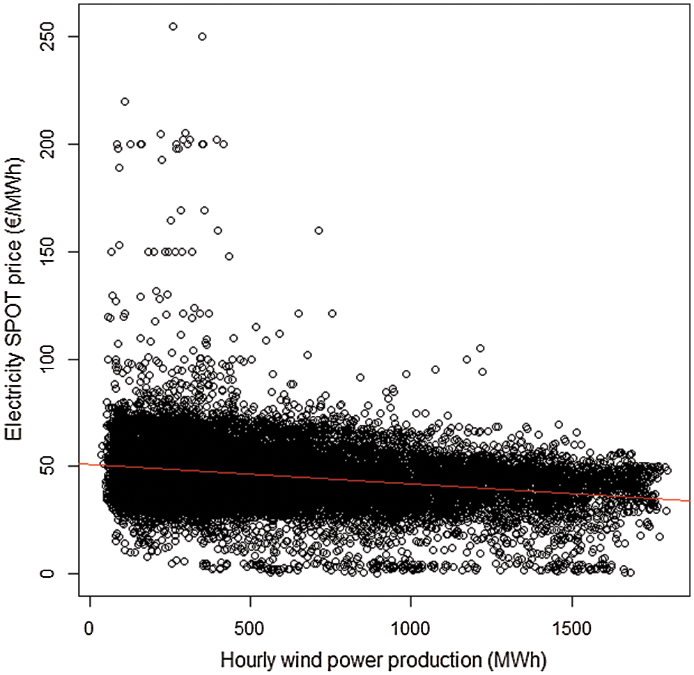
Figure 1: Relationship between hourly wind power production (hourly forecast) and electricity spot prices in Finland in 2018 and 2019. Red line is fitted to the points using least squares method [7,8]
This study compares 17 different places in Finland in terms of estimated revenue from wind power production. This is done by estimating hourly generation with three turbine types at two different hub heights and multiplying the generation with hourly electricity spot prices. By definition, two variables determine the lucrativeness of a location from the perspective of revenue: First, technical potential the location has for wind power which determines the power output and second, price in the electricity wholesale markets when electricity is generated at the location.
The first of the two variables mentioned above is rather straightforward but the second may need more explaining. Since the wholesale electricity price is the same everywhere in Finland, is not the latter variable same for every location? A reason why the second variable may differ between locations is that power output varies between locations temporally. Hence, it is possible that on average, price paid per generated unit of electricity, such as megawatt hour (MWh) varies between locations both because of random variation in price as well as power output and the relationship between wind power generation and electricity prices mentioned above. Especially, if a location has plenty of installed wind power capacity nearby, it may be that electricity price is affected by generation there which decreases the revenue from wind power generation. Schematic graph in Fig. 2 shows how this would work in theory. If the correlation graphed in Fig. 2 is real and steep enough, it is one possible way of how functional electricity markets could drive variable renewable energy generation capacity more evenly distributed spatially.
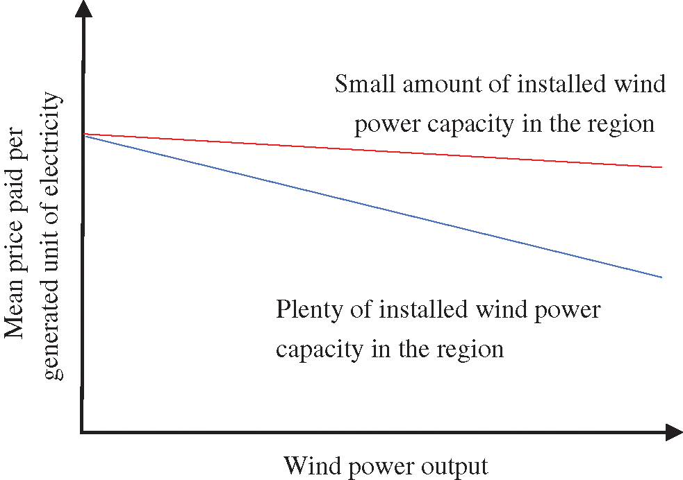
Figure 2: Schematic graph of how already installed capacity could affect revenues from wind power generation
The results of this paper are important because there are only few publicly available wind resource assessments from Finland and they are usually based on from today’s perspective old wind turbine models (see for examples [9] and [10]). In addition, to the best of our knowledge, there are no studies that combine the estimated production and electricity price at least in an hourly basis to obtain the revenue potential at different locations. Estimating potential revenues is important because as discussed earlier, the price paid per generated unit of electricity may vary between regions although the hourly electricity price was same in all the regions.
Consequently, our paper contributes to the wind resource assessment literature by providing estimates for wind power potential at several locations in Finland from the perspective of both power output and revenue from generation. Additionally, our paper contributes to the existing literature of wind power market value by providing spatially detailed estimates of mean revenue per generated MWh at locations with different levels of installed capacities in the regions.
Numerous studies have assessed technical wind power potential in different areas using rather similar methods. The assessing process is roughly visualized in Fig. 3. Wind speed data at desired locations is often gathered either from a wind atlas database, such as Finnish Wind Atlas, at a desired height as in [11] or using direct measurement data as in [12]. Direct measurements usually take place at low heights and consequently, they need to be extrapolated to wind turbine hub heights using for instance log law as in [12] and [13] or power law as in [14] where the authors analyzed these two extrapolation methodologies. Extrapolation requires information about the geography of the location, in particular about the surface roughness. This can be done by estimating surface roughness for different directions of wind, “roughness rose”, such as in [15], or using a proxy parameter for the area, which is typical for studies with large geographic scope, such as in [10].
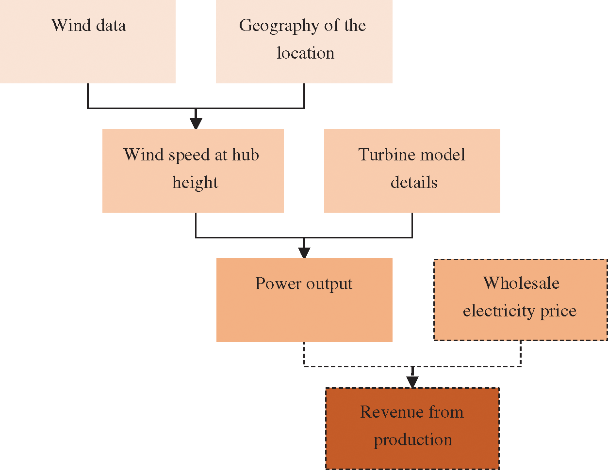
Figure 3: Wind power potential assessment process. Our contribution with a dashed line
A common method in converting extrapolated or measured wind data to power generation is by using power curve, which shows the relationship between power output and wind speed for a certain turbine. For instance, in [11] researchers carry out their estimations using several turbine types, in [16] a composite power curve derived from eight large turbine models is used and in [12] estimations are carried out using one turbine model as a representative one.
Although there are numerous studies comparing different regions in terms of wind power potential from the perspective of for example wind conditions and land use, to the best of our knowledge, there are no studies comparing potential revenues. However, for example in [6] and [5] researchers use hourly wholesale electricity price and wind power generation data to estimate the causal impact of wind power on electricity prices in different areas. That is related to the second variable determining revenue from production at a certain location: price paid for wind power production there. In addition, there is a wide economic literature estimating the market value of wind power and how it behaves as installed capacity increases under different scenarios for example for the spatial distribution of wind power capacity and carbon pricing (see for examples [17,18]). The idea behind that literature is similar to that we presented in the introduction: Increasing capacity decreases the price paid per unit of electricity generated by wind power because of the relationship between electricity price and wind power output.
Data sources for the estimations can be seen in Tab. 1
Table 1: Data sources for the estimations

Wind farms in Finland are heavily concentrated to western coastal region (Fig. 4). According to statistics provided by AFRY [1], by the end of 2019, starting from the northern part of the western coast and going towards south, North Ostrobothnia had 38.9% of cumulative capacity in Finland, Central Ostrobothnia 4.6%, Ostrobothnia 12.6%, South Ostrobothnia 10% and Satakunta 11.1%. That accounts for 77.2% of total wind power capacity. In addition, Lapland in the northern Finland had 12% of total capacity of which major share is in the northern part of the western coast. [1] Majority of planned wind farm investments are also located to the western coast (70%–80% of planned capacity), particularly to the northern part of it (Northern Ostrobothnia). Other areas of interest are Kainuu in the east and Lapland in the north, both constituting around 5% of planned capacity [3].
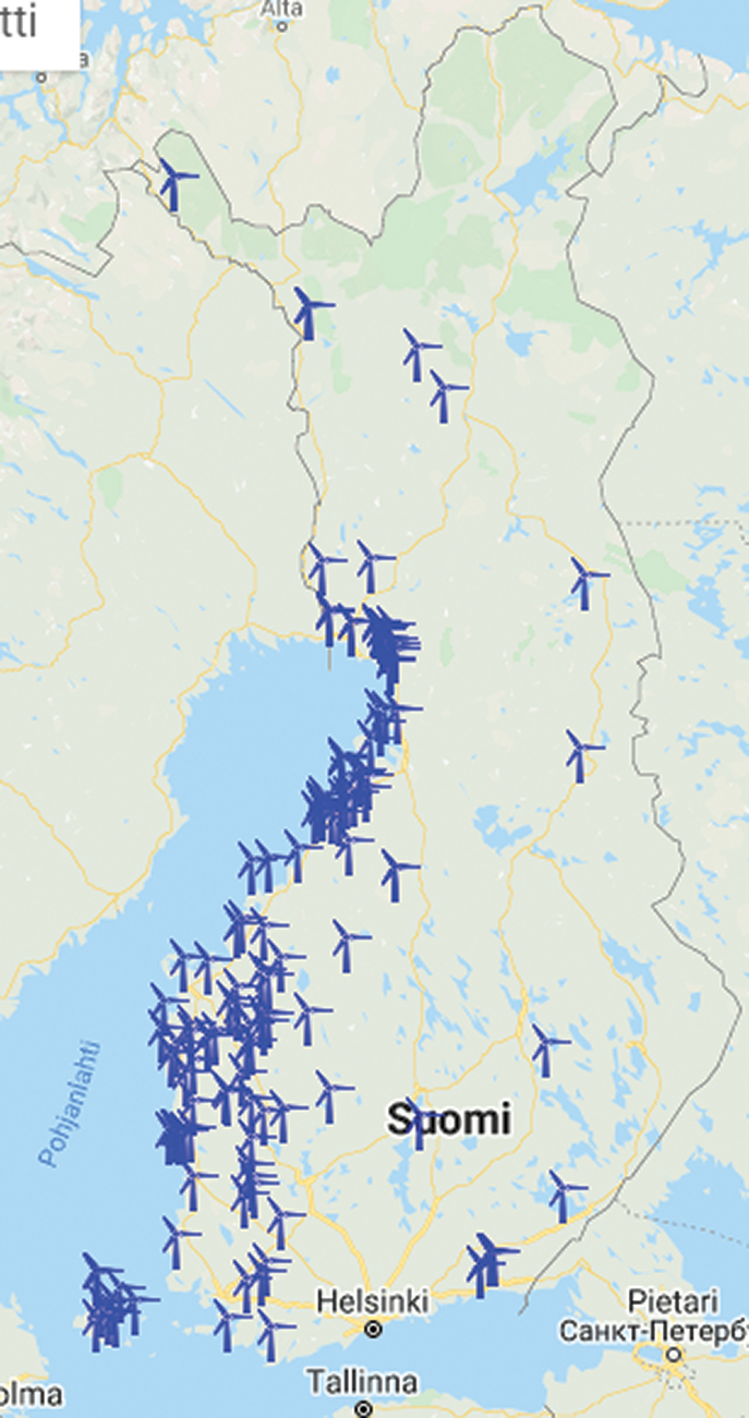
Figure 4: Map of operating wind farms in Finland [22]
Looking at the wind conditions map in Fig. 5, those areas seem to be rational choices for wind power production. Many municipalities in that area have also aging population, negative population inflow rate and low population density so in the pursuit of real estate tax revenues, they are rather avidly zoning new area for wind farms as there are also not as many obstacles to them compared to more densely populated areas [24]. However, looking at the Fig. 5, other potential areas in the southern coast as well as in elevated areas in the northern and eastern part of the country seem to be almost totally without generation. Major reason why the southern coast and practically the whole Eastern Finland are not utilized is that The Finnish Defense Forces has not allowed to install wind farms there in the fear that they would influence their radars [25]. In addition, in the Northern Finland, basic infrastructure for wind power, such as road and power grid networks, are not so good compared to more southern parts which increases construction costs there [26].
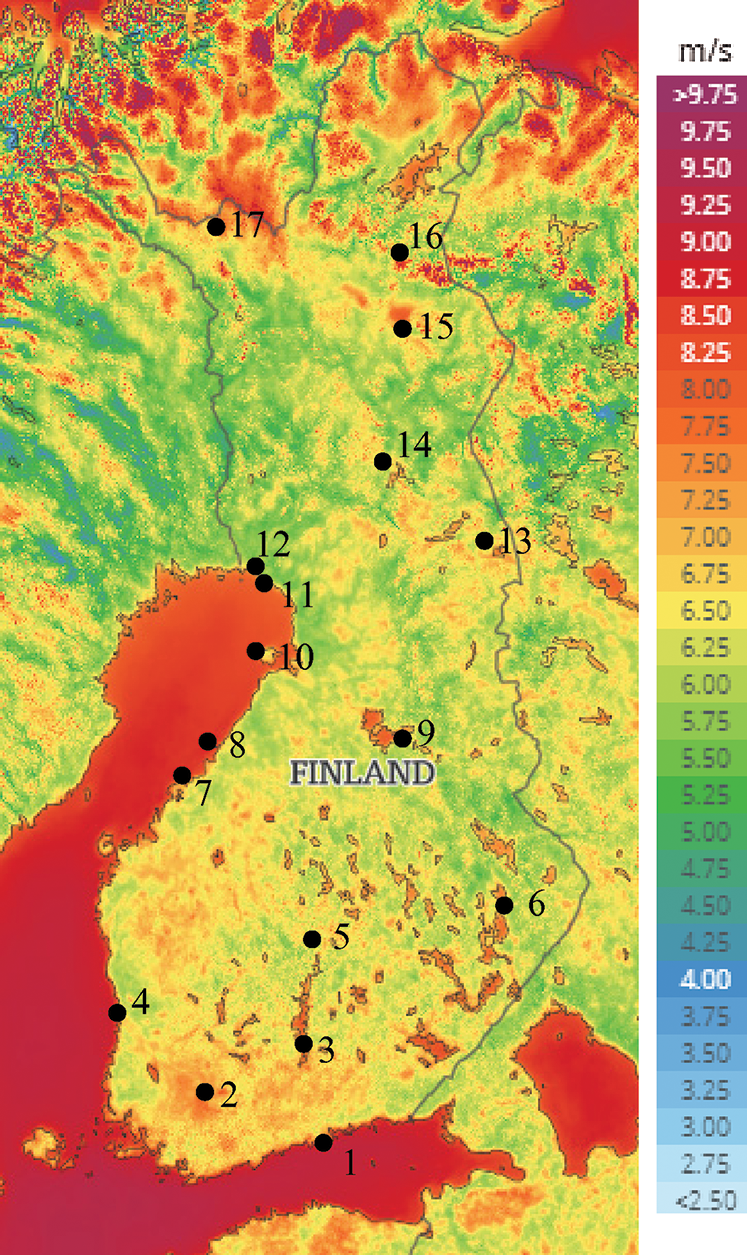
Figure 5: Map of mean wind speeds in Finland at 100 m altitude. Locations of interest are marked to the map and numbers refer to Tab. 2 [23]
Table 2: Descriptive statistics of wind data. Numbers refer to Fig. 5

In this study, 17 different locations are compared in terms of the estimated revenues from wind power production. They are marked to the map in Fig. 5. The areas have been selected based on wind conditions, already installed wind power capacity and planned wind power investments so that areas with different levels of capacity and wind conditions can be compared in terms of revenues from generation. The exact locations are the locations of weather observation stations of Finnish Meteorological Institute (FMI).
Wind speed data from FMI contains observations of average wind speed and direction in 10 min intervals covering years 2018 and 2019. Measurements are carried out 10 meters above major obstacles in the surroundings and hence, measurement heights vary between locations [27]. The heights were either obtained from Finnish Meteorological Institute [28] or if there were no information available, 15 m was used. Descriptive statistics of the wind data can be seen from Tab. 2.
Wind speeds were extrapolated to 100 m height using log law as for instance in [12]. More detailed version of that is also being used in WAsP which is generally applied tool in analyzing technical wind power potential [29]. When assuming neutral atmospheric stability and no large obstacles around the location at which wind speed is measured, relation between wind speeds at two different heights is the following:
In Eq. (1) z is the height of interest (here hub height), zr is the height in which the wind speed is measured and z0 is roughness length which is a parameter that describes land topography.
Since the parameter describing land roughness, z0, varies considerably depending on the wind direction especially on the coastal area, it was estimated separately for four cardinal directions (90° sectors) with a radius of 10 km. In Finland, roughness also differs between different periods of year mainly because of snow and ice covering land surface. Length of the period snow and ice covers the surface was assessed separately for each place using a map from Finnish Meteorological Institute Snow Statistics [30]. Base for the roughness length estimation was CORINE Land Cover 2018 raster data [21] and a roughness length table provided in Finnish Wind Atlas [10].
We had no tool for calculating exact roughness roses which may have affected the results particularly for locations that are surrounded by different types of surface coverings (for example sea and ground in the same sector). In those cases, different roughness length table values were averaged depending on how large area different surface types covered from the sector. In addition, because of the observation station in Saariselkä Kaunispää is on top of a mountain, smaller radius (−1 km) was used for it for simplicity. Tab. 3 shows roughness length values used in the simulations. Areas that differed from the prevailing surface type but had a diameter in the region of 1 km or less in the radial direction were not considered. To capture the effect of roughness length on the variables of interest (power output, and revenue), the simulation was also carried out with 30% higher and lower roughness length values.
Table 3: Roughness length values used in the estimations

To convert wind speeds at two different altitudes, 100 m and 150 m, into power output, power curves in Fig. 6 of Vestas V136 3.45 MW, Vestas V126 3.45 MW and Nordex N149 4.5 MW turbine models were obtained from thewindpower.net [20]. Since the wind observations were in 10 minutes intervals, power output was also calculated in that frequency and after that averaged for the whole hour.

Figure 6: Power curves of wind turbine models used in this study [20]
Turbine models mentioned above are used in this paper for a following reasoning: In Finland in 2019, 65% of the number of cumulative installed wind turbines had power between 3 and 3.99 MW and Vestas holds 53% of the cumulative installed capacity [1]. In addition, 91% of capacity installed in 2017 were turbines of Vestas with a power of 3.45 MW [31]. Vestas has three other turbine types with power of 3.45 MW, too, but we concentrate on these two. Model V136 is designed for low- and medium wind sites whereas V126 is for medium wind sites. Nordex N149 was chosen because in 2020, around 40% of wind farms under construction without subsidy from the state had Nordex as a turbine manufacturer and turbine power between 4.3 and 4.8 [32]. The model was chosen because there was power curve data available of it.
Besides power curves, other information about the turbines relevant in this paper can be found in Tab. 4. In the table, re cut-in wind speed means wind speed at which a turbine starts generating electricity again after cutting out due to too high wind speed. This factor has been considered for the turbines of Vestas but for Nordex N149 information about that value was not found and therefore, it was not considered.
Table 4: Detailed information of wind turbine models used in this study [33,34]

Hourly revenues were calculated by multiplying the estimated hourly production (MWh/h) with hourly electricity spot price (€/MWh/h). This was done separately for the 17 different locations and with six different combinations of turbine types and hub heights. Spot prices were obtained for Finnish bidding area from Nord Pool market data (Tab. 1 in chapter 3.1). From the estimated revenues the comparison between different locations as well as turbine models and hub heights could be made. Combining the estimated revenues and power outputs it was also possible to determine mean revenues per produced MWh using Eq. (2).
In Eq. (2)
[€/MWh] is the mean revenue per generated MWh with a given combination i of location, turbine type and hub height, gi,t [MWh] is electricity generation with a given combination i of location turbine type and hub height at a given hour t ∈ T = {1, …, t, …17520} and pt [€/MWh] is electricity spot price at a given hour t.
3.6 Electricity Price vs. Power Output Regression
To examine the relationship between electricity spot price and wind power generation at different locations, we conducted a univariate regression analysis between these two variables. We modelled the relationship as in Eq. (3) and estimated parameters β1 and β0 from our data using ordinary least squares method.
In Eq. (3) pt [€/MWh] is electricity spot price, gi,t [MWh] is wind power generation at hour t with a given combination i of location, hub height and turbine model. In addition, ɛ is an error term whereas β1 and β0 are coefficients that are to be estimated from the data.
3.7 Levelized Cost of Electricity
We also calculated estimates for levelized cost of electricity (LCOE) for every location and combination of turbine type and hub height by a modified formula from Rinne, Holttinen, Kiviluoma and Rissanen (Eq. (4)) [35].
In Eq. (4) IC is overnight investment cost (€/MW), r is interest rate, N is the power plant lifetime in years, CF is capacity factor for calculating full load hours and O&M is operations and maintenance cost (€/MW).
Fig. 7 shows the extrapolated mean wind speeds at 100 and 150 m height. As one would expect by looking at the Tab. 2 in chapter 3.3, locations on coastal area seem to have clearly the highest figures, typically between 8 and 9 m/s. However, Kemi is an exception: there the extrapolated mean wind speeds are 6.72 and 7.13 m/s at 100 and 150 m heights, respectively. At the locations in inland, mean wind speeds are typically in the region of 5 and 6 m/s with Saariselkä being an exception: There the figures are 7.94 and 8.28 m/s at 100 and 150 m height, respectively.
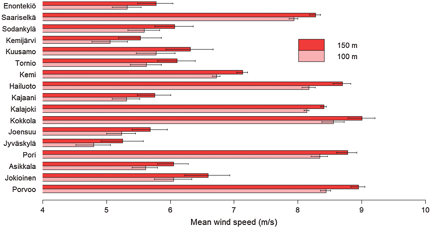
Figure 7: Extrapolated wind speeds at 100 m and 150 m height. Whisker ends represent means that are calculated using 30% higher and lower roughness length values
We also compared the estimated mean speeds at 100 m height to two other sources: Global Wind Atlas and Finnish Wind Atlas. At most locations the differences to at least one of the other sources were in the region or less than 0.5 m/s, Joensuu et al. being the clearest exceptions. There the smallest differences were 0.91 and 0.67, respectively. Differences seemed to be small especially at the locations on coastal areas, in the region of 0.3 to 0.6 m/s and again, Kemi being an exception. That is probably because in coastal areas the effect of the surface roughness on wind speed can be modelled easily (roughness length close to zero). It is also worth mentioning that these two other sources use more sophisticated methods for estimating roughness lengths than we do but because of their large geographic scope the results may not be in spatial sense as accurate as ours. In addition, their timeframe is much wider, Global Wind Atlas covers years 2008–2017 and Finnish Wind Atlas years 1989–2007, which makes them more robust against short-term variation in wind speeds [10,23].
Tab. 5 and Fig. 8 show the average power outputs and capacity factors for every location with different turbine types and hub heights. As can be expected by looking at the wind speed extrapolations, locations on the coastal area, Porvoo, Pori, Kokkola, Kalajoki and Hailuoto have the highest average power outputs with Saariselkä that locates on top of a mountain being close to these five locations. At these locations, the highest mean hourly outputs are in the region of 2.5 MWh with N149 at 150 m height and lowest at around 1.5–1.6 MWh with V126 at 100 m height. The lowest figures are at Jyväskylä, Kemijärvi and Joensuu in inland areas where the highest mean hourly outputs are 1.12, 1.32 and 1.38 MWh with N149 at 150 m height and the lowest at 0.52, 0.65 and 0.65 MWh with V126 at 100 m height, respectively.
Table 5: Mean hourly power outputs (MWh/h)


Figure 8: Capacity factors for different turbine models at different heights and locations
Between the locations, capacity factors in Fig. 8 show similar pattern as the mean hourly outputs. The highest figures are at the same locations as before, at Porvoo capacity factor is 0.60 with V136 at 150 m height, and the lowest at Jyväskylä: 0.15 with V126 at 100 m height. However, as can be expected by looking at the power curves in Fig. 6, the order between turbine types is not the same. Vestas V136 with its good performance in low-wind conditions passes Nordex N149 albeit the difference between these two models is rather small, between 0.6 and 1.8 percentage points when comparing at the same location and height. Vestas V126 as the worst-performing model has from 6.4 to 9.5 percentage points lower capacity capacity factors than V136. Moreover, Vestas V136 comes before V126 at every location even when comparing V136 at 100 m and V126 at 150 m height.
When the estimated capacity factors are compared to the average capacity factor of wind power in Finland (32.7%) [36], they look rather high. This is because our estimations are for an idealized case that does not take into account losses occuring for example because of other wind turbines nearby in a wind farm and/or icing of wind turbine blades.
We also simulated hourly outputs and capacity factors by using 30% higher and lower values for surface roughness length. As can be seen in Fig. 9 the range between these two extremes is narrow for locations on coastal areas and clearly wider for most of the locations in inland. That is because, as discussed above, the roughness length values for prevailing wind directions at the locations on coast are low, close to zero, whereas those for locations in inland are higher, typically 1.2 or 1.4. For capacity factors the width of the range between upper and lower value at the locations on coast and Saariselkä (low roughness length) is between 0.6 and 2.1 percentage points and in inland excluding Saariselkä the range is between 3.1 and 7.2 percentage points. In terms of average hourly outputs, the results can be seen in Fig. 9.

Figure 9: Difference in mean hourly power output when using 30% higher and lower values for surface roughness length
Tab. 6 shows revenue means the similar way power outputs were assessed above. When comparing to Tab. 5 that shows the average power outputs, mean revenues seem to be consistent with those. No notable difference can be detected in either the order between different locations or between turbine models and hub heights. Therefore, the highest revenues can be found at Porvoo, Pori, Kokkola, Kalajoki, Hailuoto and Saariselkä with Nordex N149 at 150 m (116.24 €/h in Porvoo) and the lowest at Jyväskylä, Joensuu and Kemijärvi with Vestas V126 at 100 m (22.92 €/h in Jyväskylä).
Table 6: Mean hourly revenues €/h

When the mean hourly revenues are calculated using 30% higher and lower values for surface roughness length as in Fig. 10, differences between the two extremes show similar pattern as for power outputs. For locations on coast and Saariselkä the differences are from 0.90 to 4.51 €/h and for locations in inland excluding Saariselkä they are from 4.94 to 14.60 €/h, and again, the widest ranges being for Nordex N149 at 150 m height.
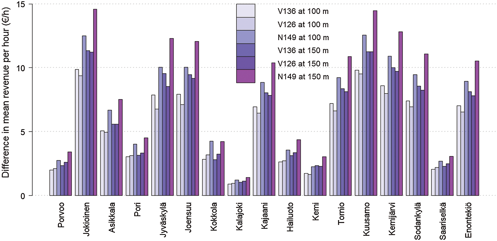
Figure 10: Difference in revenue means when using 30% higher and lower values for surface roughness length
Distributions of revenues can be seen in the boxplots of Fig. 11 that shows revenues with Nordex N149 at 150 m height. Resulting from the positive skewness of the distributions of wind speeds and hence, power outputs, revenues are positively skewed and the lower the median value (black line inside the box) the more so. In addition, when comparing mean and median values in Tab. 6 and Fig. 11, they seem to be in line between different places but as can be expected, median values are smaller.
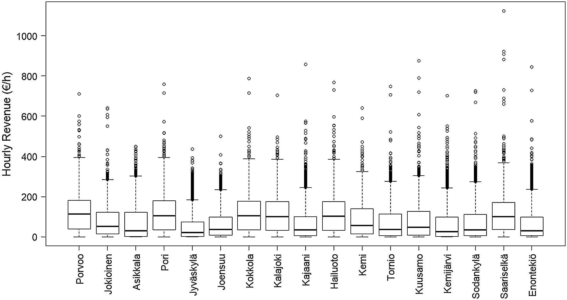
Figure 11: Boxplots of hourly revenues with Nordex N149 at 150 m height
Fig. 12 shows percentage differences between the simulated average hourly revenues and rough estimates based on simply the simulated mean hourly outputs multiplied by the mean electricity spot price over the two-year period. At every location, except at Kajaani, the rough estimates based on mean electricity price and power output are higher. The largest difference is at Kemi, 6.78% with V126 at 100 m height and on average over all locations, turbine types and hub heights, the difference is 2.8%. On hourly basis that difference is at maximum only slightly over 4 € but over the whole lifetime of a wind turbine the cumulative difference is rather large: If we hold the average hourly revenues constant over a 30-year-period and calculate net present values of total revenue over this period using these two estimates for hourly revenues, at Porvoo with V126 at 100 m height the difference between net present values is 380510.1 € using 5% discount rate.
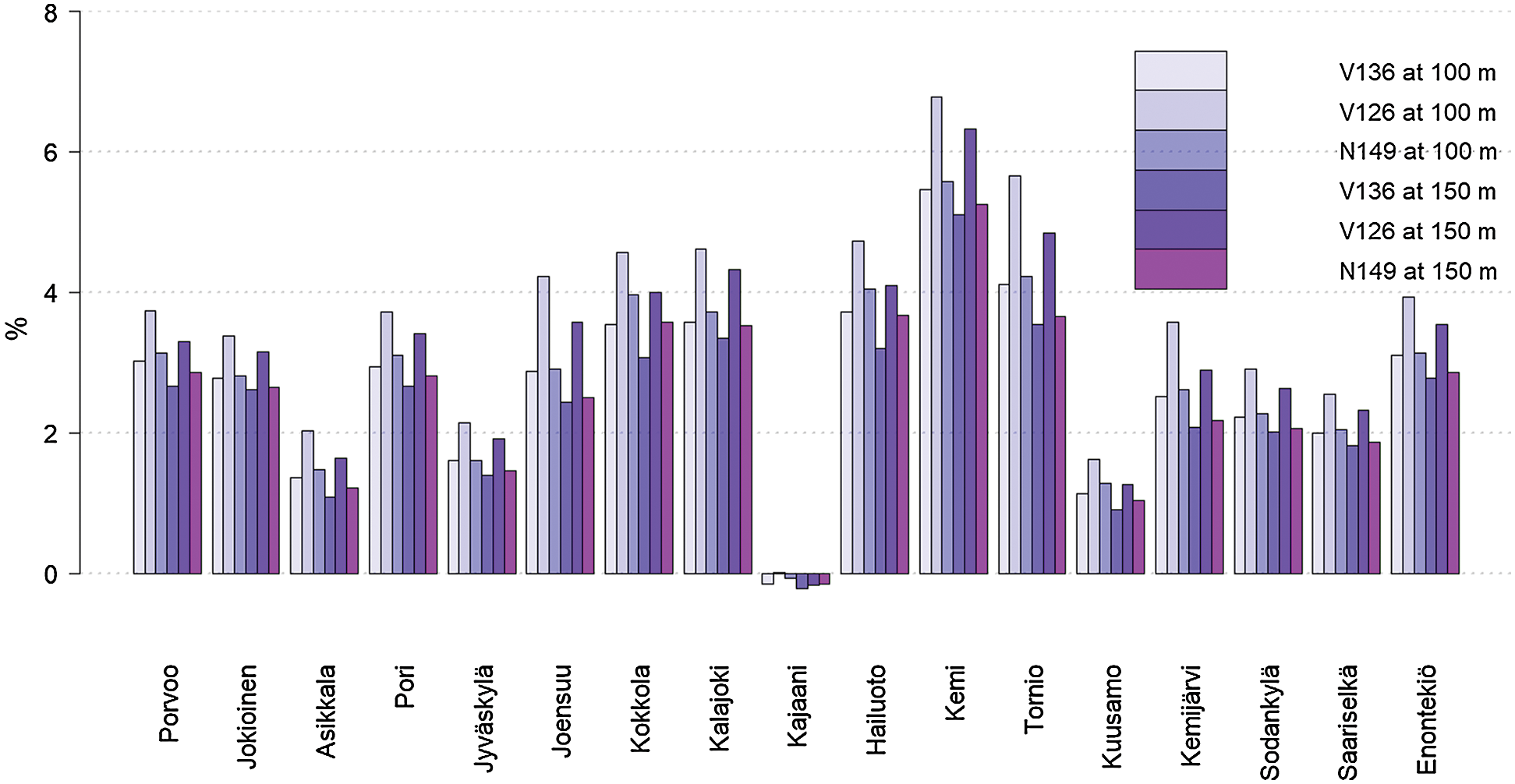
Figure 12: Difference between mean hourly revenues when calculated using mean electricity spot price multiplied by mean hourly output and the simulated mean revenues in Tab. 6
4.4 Western Coast Compared to Other Locations
This section assesses whether on average, revenue per generated unit of electricity varies between locations and if so, whether that can be attributed to already installed capacity in the region of the locations. For that use in this study, the locations on western coast (Pori, Kokkola, Kalajoki, Hailuoto, Kemi and Tornio) are compared to other locations in terms of mean revenue per generated MWh. As seen before, major share of installed wind power capacity and planned investments in Finland are located on the western coast. Hence, if we assume that all the locations are similar when it comes to other factors that may affect the results, such as generation profiles between different periods of the year, we can attribute at least part of the variation to different levels of installed capacity. However, for more reliable and detailed estimates, more locations and more detailed data of where the installed capacity is located and how much capacity is in each place should be used, but here we concentrate on assessing signs of existence of the effect. Looking at the mean revenues per hour in Tab. 6 and comparing those to the average hourly outputs in Tab. 5, it is hard to detect if there are any differences between average prices per generated unit of electricity. Pori, Kokkola, Kalajoki and Hailuoto seem to have high whereas Kemi and Tornio relatively low average hourly revenues but that is what can be expected when considering the mean hourly power outputs and wind speeds in Tab. 5 and Fig. 7. From Fig. 12 it is possible to see that there might be differences in mean price per MWh between locations and it becomes clearer in the following analysis.
Firstly, Fig. 13 shows mean revenue per generated MWh (

Figure 13: Mean revenue per generated MWh. Line represents the mean of all places with every turbine type and hub height (44.17 €/MWh). Note the shortened y axis
As a comparison, we calculated
Secondly, Fig. 14 is a result of sampling all possible combinations (12376 combinations) for two sets of locations, one with six locations and one with 11, and then calculating the

Figure 14: Density plot for differences between mean revenues per generated MWh for two sets of locations, one with six and one with 11 locations. Vertical lines show the differences when the set of six contains all the locations on the western coast
Thirdly, to examine more thoroughly the relationship between power output and electricity mean price at different locations, we conducted a regression analysis using Eq. (3) at every location with Vestas V126 at 100 m height. As an example, Fig. 15 shows the results for Kalajoki. The slope coefficient β1 takes value −1.71 €/MWh2 and the intersection term β0 is 48.16 €/MWh. R2-value that gives information about the goodness-of-fit of the regression i.e., how well the regression model explains variance in the dependent variable (electricity price) from the independent variable (power output), for this location is 0.0236. R2 gets values from 0 to 1 and a value of 1 means that the points fit perfectly to the model.

Figure 15: Relationship between mean price of electricity and power output at Kalajoki. Note the shortened y axis. Width of the interval for which the points are calculated is 0.05 MWh
Tab. 7 shows the parameters of the regressed lines for every location. As can be seen, slopes and R2s are larger in absolute terms for locations on western coast (Pori, Kokkola, Kalajoki, Hailuoto, Kemi, Tornio) than for others. The only exception is Pori, for which the slope is less steep than for Porvoo and Joensuu. In addition, R2s for Tornio and Pori are lower than for Porvoo. A likely reason why the lines are downward sloping even at locations, except Kajaani, that have no or little installed wind power capacity in the region is that wind conditions are correlated between different areas in Finland. In addition, as one could expect, R2s are relatively low since there are multiple other factors explaining the electricity price besides potential wind power generation in one are although the area had relatively large amount of installed capacity.
Table 7: Regression coefficients and R2’s

Trying to explain exactly why the relationship between power output and mean revenue per generated MWh as well as the order between locations are as analyzed above is beyond the scope of this study but the pattern seems clear: At locations on the western coast
4.5 Comparing Revenues to Cost Estimates
We calculated our estimates for LCOE using Eq. (4) applying the same parameters as Vakkilainen et al. [35]: an interest rate of 5%, power plant lifetime of 25 years, operations and maintenance costs of investment cost of a wind farm installed in coastal area (1360 €/kW) [35]. For operations and maintenance costs we used an estimate from the Finnish Wind Power Association (0.02 of the investment cost per annum) [38]. We varied only the value for capacity factor that was taken from our calculations. Of course, especially investment costs may vary considerably between different locations, wind farm sizes and turbine types but estimating those is beyond the scope of this study. However, to capture the effect of the variation in investment costs on LCOE, we also calculated LCOE values using 30% higher and 30% lower values for IC. Hence, the upper boundary for it was 1768 €/kW that is slightly larger than Rinne, Holttinen et al. [11] applied as an investment cost without location specific costs for Vestas V136 3.45 MW at 150 m height. Lower boundary was 952 €/kW which is also slightly larger than Rinne, Holttinen et al. used for Vestas V90 3.0 MW turbine at 75 m height.
Fig. 16 shows the results when the LCOE’s are subtracted from
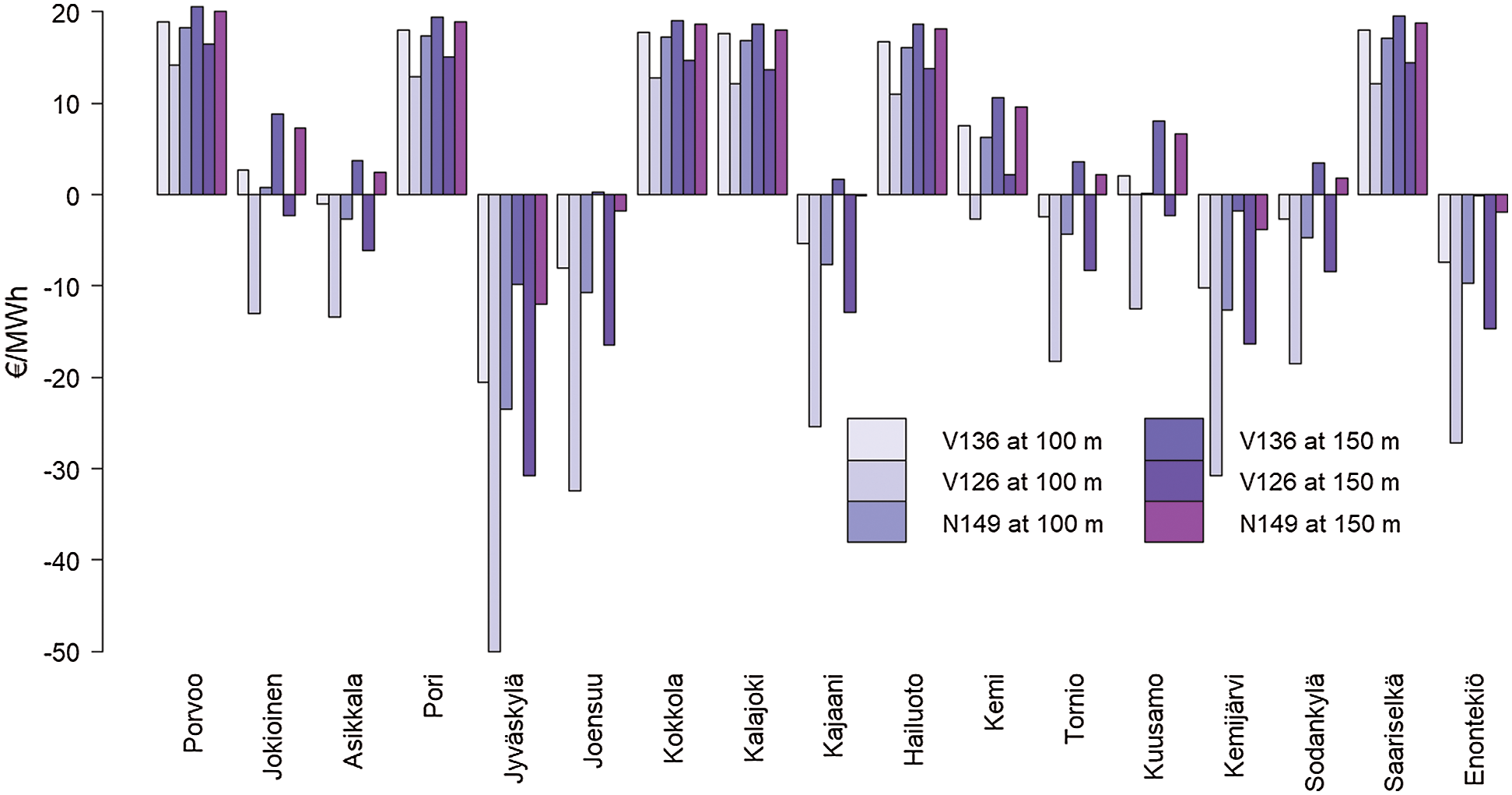
Figure 16: LCOE estimates subtracted from mean revenues per generated MWh
Impact of varying the value for investment cost on LCOE estimates increases as the capacity factor decreases. The largest difference between high- and low-end estimate for LCOE is at Jyväskylä with V126 at 100 m height (56.70 €/MWh) and the smallest is at Porvoo with V136 at 150 m height (14.22 €/MWh). On average the difference is 25.53 €/MWh. Using the low-end estimate for LCOE, according to these rough estimates, installing a wind turbine would be profitable at all locations with at least two combinations of turbine models and hub heights. With the high-end estimates installing would be profitable only at Porvoo, Pori, Kokkola, Kalajoki, Hailuoto and Saariselkä with every turbine type and at Kemi with one turbine type.
We have presented a method of how to analyze wind power potential at different locations as well as the relationship between electricity wholesale market price and wind power generation at a certain location. As seen above, from that analysis it is also possible to assess the potential profitability of a wind farm investment with a given cost structure. In addition, our method of calculating
However, our method comes with two important caveats: Being based on historical data, the results of our simulation provide only a limited amount of information when making for example investment decisions with a time horizon far into the future. As seen in Section 4.4, over the two-year period the
What can be said based on our results with a reasonably high level of confidence though, is that from the perspective of potential revenue, the best areas to install wind power in Finland are coastal regions as well as the elevated areas in the Lapland. Based on our calculations of LCOEs and
As briefly discussed in the introduction, differing mean revenues per MWh between areas is one mechanism of how functional electricity markets give investors an incentive to build capacity spatially dispersed. That is also a desirable outcome from the whole power system perspective since it helps mitigating the challenges that the intermittency of wind power generation causes for the power system [40]. Nevertheless, since investors have multiple other factors to consider besides
Table 8: Correlations between measured wind speeds (note that coefficients are multiplied by 100)

Wind power capacity in Finland is heavily concentrated on western coast because of reasons related to wind conditions, radars of The Finnish Defense Forces and zoning policy. Capacity has been growing and in the coming decade is expected to grow fast, majority of investments still being located on the western coast.
In this study we compared 17 different locations from the perspective of potential revenues from wind power production with three different wind turbine models and at two different hub heights. Estimated average hourly revenues were the largest at Porvoo Emäsalo on the southern coast, while the second and third largest were at Pori Tahkoluoto and Kokkola Tankar on the western coast, respectively. The lowest revenues were at Jyväskylä in the Central Finland.
When considering means of estimated revenues per generated MWh, we found small differences between locations. Although the differences were small, our results showed that the lowest figures were at locations on the western coast, Kemi and Tornio in the northern part of it having the lowest values. When we assessed the results more thoroughly, one likely reason why those places were at the bottom was that electricity prices are affected by generation in the region of those places because of relatively high amount of installed capacity there and on the western coast in general.
Nevertheless, at least at this stage, clearly the most important factor determining the lucrativeness of a location in terms of revenue seemed to be power output as shown in Section 4.6. In the future, considering where the upcoming investments are located in, the amount of already installed wind power capacity in the region may become an important factor, too. That is because of the negative correlation (and causal relationship) between wind power generation and electricity price discussed earlier in this study. In addition, as shown in Fig. 12, even at this stage it may be important to notice that on average, revenue per MWh generated by wind power is not equal to the average electricity spot price.
Acknowledgement: The author wants to thank teachers and professors who have educated him throughout his education and especially Dr. Ali Khosravi who was the supervisor of the Bachelor’s Thesis and with his experience contributed to this study.
Funding Statement: The authors received no specific funding for this study.
Conflicts of Interest: The authors declare that they have no conflicts of interest to report regarding the present study.
1. AFRY (2020). Wind Power in Finland 2019. https://www.tuulivoimayhdistys.fi/filebank/1457-Tuulivoimatilastot_AFRY_eng.pdf. [Google Scholar]
2. Energiateollisuus ry (2020). Energiavuosi 2019. Sähkö. https://energia.fi/files/4360/Sahkovuosi_2019_mediakuvat.pdf. [Google Scholar]
3. Etha Wind (2020). Wind Farms and Projects in Finland 2020. https://www.tuulivoimayhdistys.fi/en/wind-power-in-finland/wind-power-projects-in-finland/wind-power-projects-in-finland. [Google Scholar]
4. Nord Pool (2017). Price Calculation. https://www.nordpoolgroup.com/trading/Day-ahead-trading/Price-calculation/. [Google Scholar]
5. Quint, D., Dahlke, S. (2019). The impact of wind generation on wholesale electricity market prices in the midcontinent independent system operator energy market: An empirical investigation. Energy, 169, 456–466. DOI 10.1016/j.energy.2018.12.028. [Google Scholar]
6. Amor, M. B., Billette de Villemeur, E., Pellat, M., Pineau, P. (2014). Influence of wind power on hourly electricity prices and GHG (greenhouse gas) emissions: Evidence that congestion matters from Ontario zonal data. Energy, 66, 458–469. DOI 10.1016/j.energy.2014.01.059. [Google Scholar]
7. Fingrid (2020). Continuously Updated Wind Power Forecast. https://data.fingrid.fi/. [Google Scholar]
8. Nord Pool (2020). Historical Market Data. https://www.nordpoolgroup.com/historical-market-data/. [Google Scholar]
9. Hynynen, K. M., Baygildina, E., Pyrhönen, O. (2012). Wind resource assessment in southeast Finland. IEEE Power Electronics and Machines in Wind Applications, pp. 1–5. DOI 10.1109/PEMWA.2012.6316376. [Google Scholar]
10. FMI (2009). Finnish Wind Atlas. http://www.tuuliatlas.fi. [Google Scholar]
11. Rinne, E., Holttinen, H., Kiviluoma, J., Rissanen, S. (2018). Effects of turbine technology and land use on wind power resource potential. Nature Energy, 3, 494–500. DOI 10.1038/s41560-018-0137-9. [Google Scholar]
12. Sherida, B., Baker, S. D., Pearre, N. S., Firestone, J., Kempton, W. (2012). Calculating the offshore wind power resource: Robust assessment methods applied to the U.S. Atlantic Coast. Renewable Energy, 43, 224–233. DOI 10.1016/j.renene.2011.11.029. [Google Scholar]
13. González-Aparicio, I., Monforti, F., Volker, P., Zucker, A., Careri, F. et al. (2017). Simulating European wind power generation applying statistical downscaling to reanalysis data. Applied Energy, 199, 155–168. DOI 10.1016/j.apenergy.2017.04.066. [Google Scholar]
14. Bañuelos-Ruedas, F., Angeles-Camacho, C., Rios-Marcuello, S. (2010). Analysis and validation of the methodology used in the extrapolation of wind speed data at different heights. Renewable and Sustainable Energy Reviews, 14, 2383–2391. DOI 10.1016/j.rser.2010.05.001. [Google Scholar]
15. Gualtieri, G., Secci, S. (2011). Wind shear coefficients, roughness length and energy yield over coastal locations in Southern Italy. Renewable Energy, 36, 1081–1094. DOI 10.1016/j.renene.2010.09.001. [Google Scholar]
16. Bosch, J., Staffell, I., Hawkes, A. D. (2017). Temporally-explicit and spatially-resolved global onshore wind energy potentials. Energy, 131, 207–217. DOI 10.1016/j.energy.2017.05.052. [Google Scholar]
17. Hirth, L. (2013). The market value of variable renewables: The effect of solar wind power variability on their relative price. Energy Economics, 38, 218–236. DOI 10.1016/j.eneco.2013.02.004. [Google Scholar]
18. Eising, M., Hobbie, H., Möst, D. (2020). Future wind and solar power market values in Germany—Evidence of spatial and technological dependencies? Energy Economics, 86, 104638. DOI 10.1016/j.eneco.2019.104638. [Google Scholar]
19. FMI (2020). Download Observations. https://www.ilmatieteenlaitos.fi/havaintojen-lataus. [Google Scholar]
20. The Wind Power (2020). Manufacturers and Turbines. https://www.thewindpower.net/turbines_manufacturers_en.php. [Google Scholar]
21. National Land Survey of Finland, Finnish Environment Institute (2019). Paikkatietoikkuna-CORINE MAANPEITE 2018. https://kartta.paikkatietoikkuna.fi. [Google Scholar]
22. Etha Wind & Finnish Wind Power Association (2019). Finnish Wind Farms. https://www.ethawind.com/suomen-tuulivoimapuistot. [Google Scholar]
23. World Bank & Technical University of Denmark (2019). Global Wind Atlas. https://globalwindatlas.info. [Google Scholar]
24. Mainio, T. (2019). Tuulivoima tuo isäntäkunnille jopa miljoonatulot kiinteistöveroina. https://kuntalehti.fi/uutiset/talous/tuulivoima-tuo-isantakunnille-jopa-miljoonatulot-kiinteistoveroina/. [Google Scholar]
25. Pyrhönen, O., Partanen, J., Vakkilainen, E., Hynynen, K. (2019). Tuulivoiman tutkahäiriökysymys on ratkaistava osana hävittäjähankintoja. https://www.lut.fi/uutiset/-/asset_publisher/h33vOeufOQWn/content/tuulivoiman-tutkahairiokysymys-on-ratkaistava-osana-havittajahankintoja. [Google Scholar]
26. Fingrid (2020). Karttapalvelu. https://fingrid.navici.com. [Google Scholar]
27. Finnish Meteorological Institute (2016). Havaintosuureet. https://www.ilmatieteenlaitos.fi/havaintosuureet. [Google Scholar]
28. Finnish Meteorological Institute (2020). Havaintoasemat. https://www.ilmatieteenlaitos.fi/havaintoasemat. [Google Scholar]
29. Serny Jacobsen, H. (2014). Frequently Asked Questions-WaSP. https://www.wasp.dk/support/faq. [Google Scholar]
30. Finnish Meteorological Institute (2012). Snow Statistics. https://en.ilmatieteenlaitos.fi/snow-statistics. [Google Scholar]
31. Finnish Wind Power Association (2019). List of Wind Farms in Production. https://www.tuulivoimayhdistys.fi/en/wind-power-in-finland/wind-power-projects-in-finland/wind-power-projects-in-finland. [Google Scholar]
32. Finnish Wind Power Association (2020). Projects under Construction. https://tuulivoimayhdistys.fi/en/wind-power-in-finland/projects-under-construction. [Google Scholar]
33. Vestas (2020). 4MW PLATFORM. http://nozebra.ipapercms.dk/Vestas/Communication/Productbrochure/4MWbrochure/4MWProductBrochure/?page=20. [Google Scholar]
34. Nordex (2020). N149/4.0-4.5. https://www.nordex-online.com/en/product/n149-4-0-4-5/. [Google Scholar]
35. Vakkilainen, E., Kivistö, A. (2017). Comparison of Electricity Production Costs. http://urn.fi/URN:ISBN:978-952-335-124-0. [Google Scholar]
36. VTT (2019). Wind Statistics 2018. https://www.tuulivoimayhdistys.fi/filebank/1398-Wind_Statistics_2018_Public.pdf. [Google Scholar]
37. ENTSO, E. (2020). Actual Generation per Production Type. https://transparency.entsoe.eu/generation/r2/actualGenerationPerProductionType/show. [Google Scholar]
38. Finnish Wind Power Association (2020). Käyttö- ja ylläpitokustannukset. https://tuulivoimayhdistys.fi/tietoa-tuulivoimasta-2/tietoa-tuulivoimasta/taloudellisuus/kaytto-ja-yllapitokustannukset. [Google Scholar]
39. Svenska Kraftnät (2019). Långsiktig marknadsanalys 2018. https://www.svk.se/siteassets/om-oss/rapporter/2019/langsiktig-marknadsanalys-2018_sammanfattning.pdf. [Google Scholar]
40. Ren, G., Liu, J., Wan, J., Guo, Y., Yu, D. (2017). Overview of wind power intermittency: Impacts, measurements, and mitigation solutions. Applied Energy, 204, 47–65. DOI 10.1016/j.apenergy.2017.06.098. [Google Scholar]
 | This work is licensed under a Creative Commons Attribution 4.0 International License, which permits unrestricted use, distribution, and reproduction in any medium, provided the original work is properly cited. |