| Energy Engineering |
DOI: 10.32604/EE.2021.014961
ARTICLE
An Intelligent Diagnosis Method of the Working Conditions in Sucker-Rod Pump Wells Based on Convolutional Neural Networks and Transfer Learning
1Shengli College China University of Petroleum, Dongying, 257061, China
2China University of Petroleum (East China), Qingdao, 266580, China
*Corresponding Author: Ruichao Zhang. Email: zrcupc@slcupc.edu.cn
Received: 11 November 2020; Accepted: 12 December 2020
Abstract: In recent years, deep learning models represented by convolutional neural networks have shown incomparable advantages in image recognition and have been widely used in various fields. In the diagnosis of sucker-rod pump working conditions, due to the lack of a large-scale dynamometer card data set, the advantages of a deep convolutional neural network are not well reflected, and its application is limited. Therefore, this paper proposes an intelligent diagnosis method of the working conditions in sucker-rod pump wells based on transfer learning, which is used to solve the problem of too few samples in a dynamometer card data set. Based on the dynamometer cards measured in oilfields, image classification and preprocessing are conducted, and a dynamometer card data set including 10 typical working conditions is created. On this basis, using a trained deep convolutional neural network learning model, model training and parameter optimization are conducted, and the learned deep dynamometer card features are transferred and applied so as to realize the intelligent diagnosis of dynamometer cards. The experimental results show that transfer learning is feasible, and the performance of the deep convolutional neural network is better than that of the shallow convolutional neural network and general fully connected neural network. The deep convolutional neural network can effectively and accurately diagnose the working conditions of sucker-rod pump wells and provide an effective method to solve the problem of few samples in dynamometer card data sets.
Keywords: Sucker-rod pump well; dynamometer card; convolutional neural network; transfer learning; working condition diagnosis
Currently, most oilfields have entered the middle and late stages of development; hence, the production benefits are increasingly low [1–4]. The sucker-rod pump is the main pumping system that provides mechanical energy for oil production [5–8], but due to abnormal working conditions and inefficient management, the energy consumption of production is large [9–10]. Therefore, the timely diagnosis and analysis of the production system is important to ensure the safe operation of oil wells and the maximization of the economic benefits of oilfield development [11–12]. Dynamometer card analysis is an important means and effective measure to diagnose the working conditions of sucker-rod pumps [13–15]. However, with the informatization construction of oilfields, dynamometer cards have realized online real-time acquisition [16]. The traditional manual analysis method is difficult to popularize because it needs considerable manpower and material resources and is affected by professional experience. Due to the good nonlinear approximation ability of artificial neural networks, back propagation neural networks [17], radial basis function neural networks [18], wavelet neural networks [19], extreme learning machines [20], self-organizing neural networks [21,22] and other models have been applied to the working condition diagnosis of sucker-rod pump wells and are gradually replacing traditional manual analysis methods. However, limited by the mechanism of the model, these methods have the following problems: (1) The input of the model is hundreds of load and displacement data measurements, which makes the internal mapping structure of the model complex and seriously affects the diagnostic accuracy of the model [23]; (2) The working condition diagnosis is based on the shape feature of a dynamometer card, and the input of load and displacement data makes the model unable to extract the shape feature of the dynamometer card directly and effectively.
In recent years, with the continuous emergence of large-scale data sets and the continuous improvement of computer GPU computing power, deep learning models represented by convolutional neural networks, such as AlexNet [24], GoogLeNet [25], VGG-16 [26], ResNet [27] and DenseNet [28], have shown incomparable advantages in image recognition. These excellent neural network models provide the basis for the identification and diagnosis of dynamometer cards. A deep convolutional neural network needs a large number of data samples for training to optimize millions of parameters to complete the accurate classification of targets. However, due to the factors of data acquisition, dynamometer card classification and quality control, it is very difficult to obtain a dynamometer card data set with millions of samples. Therefore, the deep convolutional neural network model is applied to the ImageNet image data set for pretraining, and the trained model is applied to the dynamometer card data set to optimize the parameters so as to realize the intelligent diagnosis of the working conditions in sucker-rod pump wells. This method can be applied to a dynamometer card data set with few samples without overfitting occurring. The method expands the application range of deep convolutional neural networks and provides a new method and idea for the working condition diagnosis of sucker-rod pump wells.
2.1 Establishment of the Dynamometer Card Dataset
2.1.1 Data Acquisition and Classification
The data set studied in this paper comes from the measured dynamometer cards of sucker-rod pump wells in an oilfield. According to the graphic features and production experience, the dynamometer cards are classified. There are many types of dynamometer cards. In this paper, only ten common types are selected for analysis, as shown in Tab. 1. The obtained data set contains 7000 dynamometer cards, which are divided into a training set, a verification set and a test set at a ratio of 8:1:1, that is, the training set contains 5600 dynamometer cards, the verification set contains 700 dynamometer cards and the test set contains 700 dynamometer cards.
Table 1: Classification of dynamometer cards

The obtained dynamometer card images cannot be directly used as the input images of a convolutional neural network, so the images need to be preprocessed. Preprocessing can standardize the dynamometer card images and improve the stability and accuracy of dynamometer card classification and recognition. Dynamometer card diagnosis mainly identifies the shape features of dynamometer cards. Colour information is useless for the shape recognition of dynamometer cards and to a certain extent increases the complexity of the background. Therefore, this paper binarizes the original dynamometer card images and cuts them to 96 × 96. Next, zero mean normalization is conducted to improve the optimization efficiency of the algorithm and accelerate the convergence of the model. Finally, the number of samples is increased by rotating and mirroring images to reduce the overfitting problem in the deep learning process so as to improve the generalization performance of the diagnosis model. After rotating and mirroring images, the sample size can be expanded to 8 times the original size. The data preprocessing flow of dynamometer cards is shown in Fig. 1.

Figure 1: Preprocessing of dynamometer cards
2.2 Transfer Deep Learning Network
The AlexNet network won the ILSVRC competition in 2012 with a large score. Its top-5 error rate was only 17%, far lower than the 26% of the second place method. It is similar to the LeNet-5 network architecture but larger and deeper than the LeNet-5 network. The model has 60 million parameters and 650000 neurons. It is composed of five convolutional layers (some convolutional layers are followed by pooling layers) and three fully connected layers, as shown in Fig. 2.

Figure 2: AlexNet network architecture
In order to improve the training speed, the AlexNet model introduces the ReLU modified linear element activation function, which greatly shortens the learning period [29]. Second, in order to reduce overfitting, the AlexNet model uses an elimination strategy (the elimination rate is 50%) and uses various offsets, horizontal flips and other methods to randomly move training data. In addition, the local response normalization function is also used in the AlexNet model to make different feature maps specialized, promote their separation, force them to explore new functions, and finally improve their generalization.
The GoogLeNet network won the 2014 ILSVRC competition [30] by reducing the top-5 error rate to 7%. Overall, GoogLeNet is a 27-layer deep learning network with approximately 500000 parameters, which is deeper than the AlexNet network (22 layers), but the number of parameters to be optimized is only 1/12 that of the AlexNet network. In order to avoid vanishing gradients, the model uses two different cost functions at different depths. In terms of width, the model proposes the Inception architecture, which can express information at multiple scales. The Inception architecture is shown in Fig. 3.

Figure 3: Inception architecture of the GoogLeNet network
Technically, the GoogLeNet model uses a fixed filter to conduct multiscale analysis [31], which is used for the learning of the inception structure. Additionally, GoogLeNet uses the 1 × 1 convolution method to increase the network depth and reduce the feature dimension. Finally, GoogLeNet uses the multilevel analysis method [32] and integrates the feature information of different depths to improve the recognition accuracy. Compared with the AlexNet network, the GoogLeNet network is deeper and wider, the results have been further improved, and the number of parameters is lower.
2.3.1 Hardware and Software Platform
The hardware and software platform used in this experiment is the following: Win10 64 bit, Intel i7-10700, CPU @ 4.80 GHz, 16 GB of memory, an SSD, and Python 3.2.3 Spyder.
2.3.2 Network Design of the CNN3 Model, CNN2 Model and FC Model
In addition to the above two deep convolutional neural networks, other network models, including shallow convolutional neural networks (CNN3 model and CNN2 model) and a fully connected neural network model (FC model), are designed for training. In these models, in addition to the input layer and output layer, the CNN3 model also includes two convolutional layers, two pooling layers and one fully connected layer, and the softmax function is used in the output layer. The network architecture of the CNN3 model is shown in Fig. 4. Correspondingly, the CNN2 model has one convolutional layer and one pooling layer less than the CNN3 model. The network architecture of the CNN2 model is shown in Fig. 5.

Figure 4: CNN3 network architecture

Figure 5: CNN2 network architecture
In addition, the FC model has only one fully connected layer in addition to the input layer and the output layer. The network architecture of the FC model is shown in Fig. 6.
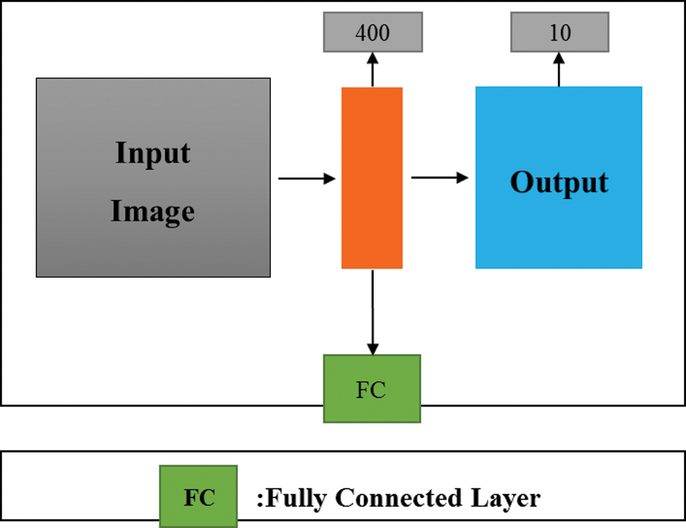
Figure 6: FC network architecture
Based on the AlexNet model and GoogLeNet model, which are pretrained using the ImageNet data set, we change the 103 nodes of the softmax output layer into 10 nodes, which are used to classify dynamometer cards under different working conditions. Then, training, verification and testing are conducted using different dynamometer card data sets. The parameters of the model network are set using a continuous optimization process. The final parameters are as follows: The initial learning rate is 0.001, the momentum factor is 0.9, the attenuation parameter is 0.0005, and the other parameters remain unchanged. Moreover, the shallow convolutional neural networks (CNN3 model and CNN2 model) and fully connected neural network model (FC model) are also trained using the dynamometer card data set. The training processes are shown in Figs. 7 and 8.

Figure 7: The training accuracy and loss
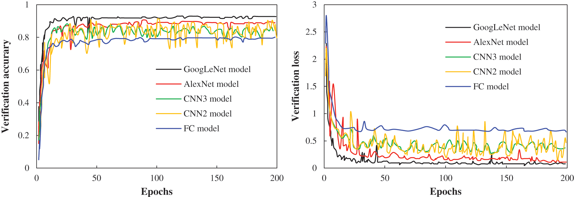
Figure 8: The verification accuracy and loss
Through training, the GoogLeNet model converges after 175 learning epochs, and the convergence time is 145276 s. The AlexNet model converges after 142 learning epochs, and the convergence time is 117862 s. The CNN3 model converges after 185 learning epochs, and the convergence time is 9745 s. The CNN2 model converges after 180 learning epochs, and the convergence time is 9281 s. Finally, the FC model converges after 115 learning epochs, and the convergence time is 6078 s.
3.1.1 Comparison of the Diagnostic Performance
The relevant experimental parameters of the number of epochs to achieve convergence, convergence time, training loss, training accuracy, verification loss and verification accuracy in the five model experiments are collected. The detailed results are shown in Tab. 2.


Figure 9: ACCs of different models

Figure 10: AUCs of different models
The diagnostic accuracies of different network models are shown in Fig. 9. Among the models, the transfer GoogLeNet network model has the highest accuracy rate of 0.92; the transfer AlexNet network model has the second highest accuracy rate of 0.89; the CNN3 network model and CNN2 network model have the third and fourth highest rates, respectively; and the FC model has the lowest accuracy at only 0.78. The results show that the prediction accuracy of the deep convolutional neural network model is higher than that of the shallow convolutional neural network and the traditional fully connected neural network model.
Cause analysis: According to the experimental results, the verification error of the deep convolutional neural network model conforms to the trend of the training error and has little fluctuation, which indicates that the model is in a good state and can effectively extract the characteristics of dynamometer cards under different working conditions. The verification error of the shallow convolutional neural network model basically conforms to the trend of the training error, but the difference is large, and the verification fluctuates violently. The loss of the model is also high. Therefore, although the model can converge, the accuracy is not high. Considering that this may be caused by the small capacity of the model, the complexity of the model can be improved, and the fitting ability of the model can be enhanced. While the fully connected neural network model can converge well, the error and loss are high, and the feature extraction ability is poor.
In addition, considering the imbalance of sample categories, it is necessary to determine the stability of different models. The AUC is the area under the ROC curve, and the value is between 0.5 and 1. The closer its value is to 1, the better the stability of the model. Therefore, we assume that one type of working condition is positive and the other is negative. Then, the average AUC of different models is calculated to determine the performance of different models. The results are shown in Tab. 3. As shown in Fig. 10, the AUC of the transfer GoogLeNet model is 0.88, the AUCs of the transfer AlexNet model and CNN3 model follow, and the AUC of the traditional fully connected neural model is lower than 0.7.
Table 3: Calculation results of the AUC

The ROC curve is also known as the sensitivity curve. It takes the true positive rate (TPR) as the ordinate and the false positive rate (FPR) as the abscissa. The ROC curve focuses on positive and negative samples at the same time, so it is more robust to the imbalance of sample categories, which is also one of the main indexes to measure the stability of the model. The closer the ROC curve is to the upper left corner, the better the performance of the model. The average ROC curves of the three diagnostic models with dynamometer card diagnostic performance better than 0.80 are shown in Fig. 11. Among the curves, green is the GoogLeNet model, red is the AlexNet model, and blue is the CNN3 model. Overall, the diagnosis performance of the GoogLeNet model is better than that of the AlexNet model and CNN3 model, which shows that transfer learning is feasible.

Figure 11: Average ROC curves of different models
3.1.3 Field Application Analysis
To further verify the practicability and accuracy of the transfer deep convolutional neural network models (GoogLeNet model and AlexNet model), 300 oil wells in the Shengli Oilfield in China were diagnosed and analysed. The results are shown in Tab. 4. The table shows that the average diagnostic accuracy of the GoogLeNet model is 90.6% and that of the AlexNet model is 88.7%, indicating that the deep convolutional neural network model based on transfer learning has higher diagnostic accuracy and performance. Therefore, GoogLeNet can be used as the method and basis for the intelligent diagnosis of sucker-rod pump wells.

(1) In the actual production of oilfields, there are many types of dynamometer cards, and the intelligent diagnosis model of the working conditions can only diagnose the 10 oil well working conditions listed in this paper. However, the research ideas and methods of this paper can be used as a reference to establish dynamometer card data sets under more types of working conditions and conduct training so as to expand the scope of working condition diagnosis. In addition, actual dynamometer cards may contain a variety of working condition information, but this working condition diagnosis model can only diagnose a certain main working condition type. Therefore, dynamometer cards under such multiple working conditions can be trained as a new type so as to realize the multicondition diagnosis of dynamometer cards.
(2) The diagnostic accuracy of the intelligent diagnosis model can be further improved. First, the data from the feature extraction is not only from used dynamometer cards but also combined with the production data of oil wells, such as daily fluid production, dynamic liquid level, and other data. These features or information can feed back the working conditions of oil wells from different levels and angles so as to make a more comprehensive and accurate diagnosis. Second, a comprehensive system of classifiers can be constructed, and the voting mechanism can be used to count the diagnosis results of different classifiers so as to realize more accurate classification of dynamometer cards. Finally, the quality and quantity of data can be improved by expanding the sample size of the dynamometer card or using data preprocessing methods such as image clipping, image quality enhancement and image flipping so as to improve the diagnostic accuracy of the working condition intelligent diagnosis model.
(1) Through the classification and preprocessing of dynamometer card data measured in oilfields, a dynamometer card data set including ten typical working conditions is established and used to train and optimize the working condition diagnosis model of sucker-rod pump wells.
(2) This paper proposes a transfer learning-based intelligent diagnosis method of the working conditions of sucker-rod pump wells, which can handle the small sample dynamometer card data set. Using the dynamometer card data set and the trained deep convolutional neural network model, model training and parameter optimization are conducted, and the learned features of the dynamometer card are transferred and applied so as to realize the intelligent diagnosis of the working conditions. The experimental results show that transfer learning is feasible and can provide methods and ideas for the intelligent diagnosis of the working conditions of sucker-rod pump wells. However, it is worth noting that a large number of parameters to be optimized will lead to the need for considerable time and computing resources for transfer deep learning.
(3) The field application results show that the deep convolutional neural network model based on transfer learning has higher diagnostic accuracy and can identify and diagnose dynamometer cards under different working conditions efficiently and accurately, which greatly improves the timeliness of oil well analysis and is conducive to improving the production efficiency and benefits of oilfields.
Funding Statement: The authors received no specific funding for this study.
Conflicts of Interest: The authors declare that they have no conflicts of interest to report regarding the present study.
1. Sun, Z. F., Lin, C. Y., Du, D. X., Bi, H. S., Ren, H. Q. (2019). Application of seismic architecture interpretation in enhancing oil recovery in late development stage—Taking meandering river reservoir in dongying depression as an example. Journal of Petroleum Science and Engineering, 187, 106769. [Google Scholar]
2. Han, D. K. (2010). Discussions on concepts, countermeasures and technical routes for the secondary development of high water-cut oilfields. Petroleum Exploration and Development, 37(5), 583–591. DOI 10.1016/S1876-3804(10)60055-9. [Google Scholar] [CrossRef]
3. Galimov, I. F., Gubaidullin, F. A., Vakhin, A. V., Isaev, P. V. (2018). Analyzing effectiveness of the terrigenous reservoirs hydrofracturing at South-Romashkinskaya area of Romashkinskoe oil field at the late stage of development (Russian). Oil Industry Journal, (1), 52–54. [Google Scholar]
4. Chen, D. C., Yao, Y., Han, H., Fu, G., Song, T. J. et al. (2016). A new prediction model for critical liquid-carrying flow rate of directional gas wells. Natural Gas Industry, 36(6), 40–44. [Google Scholar]
5. Zheng, B. Y., Gao, X. W., Li, X. Y. (2019). Diagnosis of sucker rod pump based on generating dynamometer cards. Journal of Process Control, 77, 76–88. DOI 10.1016/j.jprocont.2019.02.008. [Google Scholar] [CrossRef]
6. Bello, O., Dolberg, E. P., Teodoriu, C., Karami, H., Karami, H. et al. (2020). Transformation of academic teaching and research: Development of a highly automated experimental sucker rod pumping unit. Journal of Petroleum Science and Engineering, 190, 107087. DOI 10.1016/j.petrol.2020.107087. [Google Scholar] [CrossRef]
7. Yin, J. J., Sun, D., Yang, Y. S. (2020). A novel method for diagnosis of sucker-rod pumping systems based on the polished-rod load vibration in vertical wells. SPE Journal, 25(5), 2470–2481. DOI 10.2118/201228-PA. [Google Scholar] [CrossRef]
8. Chen, D. C., Yao, Y., Zhang, R. C., Xu, Y. X., Li, Q. et al. (2017). A new model based on pump diagram for measuring liquid production rate of oil wells in real-time. Bulletin of Science and Technology, 33(11), 77–81. [Google Scholar]
9. Zhang, R. C., Wang, Z. L., Wang, X. H., Wang, J. C., Zhang, G. Z. et al. (2018). Integrated diagnostics method and application of ground and downhole working condition in rod pumping well. Journal of Applied Science and Engineering, 24(4), 615–624. [Google Scholar]
10. Ounsakul, T., Rittirong, A., Kreethapon, T., Toempromraj, W., Rangsriwong, P. (2019). Data-driven diagnosis for artificial lift pump’s failures. SPE/IATMI Asia Pacific Oil & Gas Conference and Exhibition, Bali, Indonesia. [Google Scholar]
11. Carpenter, C. (2020). Dynamometer-card classification uses machine learning. Society of Petroleum Engineers, 72(3), 52–53. [Google Scholar]
12. Abdalla, R., Abu El Ela, M., El-Banbi, A. (2020). Identification of downhole conditions in sucker rod pumped wells using deep neural networks and genetic algorithms. SPE Production & Operations, 35(2), 435–447. DOI 10.2118/200494-PA. [Google Scholar] [CrossRef]
13. Chen, D. C., Xiao, L. F., Zhang, R. C., Yao, Y., Peng, Y. D. et al. (2017). A diagnosis model on working condition of pumping unit in oil wells based on electrical diagrams. Journal of China University of Petroleum (Edition of Natural Science), 41(2), 108–115. [Google Scholar]
14. Zhang, R. C., Yin, Y. Q., Xiao, L. F., Chen, D. C. (2020). A real-time diagnosis method of reservoir-wellbore-surface conditions in sucker-rod pump wells based on multidata combination analysis. Journal of Petroleum Science and Engineering, 198, 108254. [Google Scholar]
15. Wibawa, R., Handjoyo, T., Prasetyo, J., Purba, M., Wilantara, D. et al. (2019). Dynamometer card classification using case-based reasoning for rod pump failure identification. SPE/IATMI Asia Pacific Oil & Gas Conference and Exhibition, Bali, Indonesia. [Google Scholar]
16. Chen, D. C., Zhang, R. C., Meng, H. X., Xie, W. X., Wang, X. H. (2015). The study and application of dynamic liquid lever calculation model based on dynamometer card of oil wells. Science Technology and Engineering, 15(32), 32–35. [Google Scholar]
17. Jami, A., Heyns, P. S. (2018). Impeller fault detection under variable flow conditions based on three feature extraction methods and artificial neural networks. Journal of Mechanical Science and Technology, 32(9), 4079–4087. [Google Scholar]
18. Yu, D. L., Li, Y. M., Sun, H., Ren, Y. L., Zhang, Y. M. et al. (2017). A fault diagnosis method for oil well pump using radial basis function neural network combined with modified genetic algorithm. Journal of Control Science and Engineering, 2017(24), 1–7. DOI 10.1155/2017/5710408. [Google Scholar] [CrossRef]
19. Wu, W., Sun, W. L., Wei, H. X. (2011). A fault diagnosis of suck rod pumping system based on wavelet packet and RBF network. Advanced Materials Research, 189–193, 2665–2669. DOI 10.4028/www.scientific.net/AMR.189-193.2665. [Google Scholar] [CrossRef]
20. Li, K., Han, Y., Wang, T. (2018). A novel prediction method for down-hole working conditions of the beam pumping unit based on 8-directions chain codes and online sequential extreme learning machine. Journal of Petroleum Science and Engineering, 160, 285–301. DOI 10.1016/j.petrol.2017.10.052. [Google Scholar] [CrossRef]
21. Xu, P., Xu, S. J., Yin, H. W. (2006). Application of BP neural network and self-organizing competitive neural network to fault diagnosis of suck rod pumping system. Acta Petrol Sinica, 27(2), 107–110. [Google Scholar]
22. Liu, J., Jaiswal, A., Yao, K. T., Raghavendra, C. S. (2015). Autoencoder-derived features as inputs to classification algorithms for predicting well failures. SPE Western Regional Meeting, Garden Grove, California, USA. [Google Scholar]
23. Du, J., Liu, Z. G., Song, K. P., Yang, E. L. (2020). Fault diagnosis of pumping unit based on convolutional neural network. Journal of University of Electronic Science and Technology of China, 49(5), 751–757. [Google Scholar]
24. Krizhevsky, A., Sutskever, I., Hinton, G. (2017). ImageNet classification with deep convolutional neural networks. Communications of the ACM, 60(6), 84–90. DOI 10.1145/3065386. [Google Scholar] [CrossRef]
25. Szegedy, C., Liu, W., Jia, Y., Sermanet, P., Reed, S. et al. (2015). Going deeper with convolutions. 2015 IEEE Conference on Computer Vision and Pattern Recognition (CVPR),pp. 1–9. Boston, MA, USA. http://ieeexplore.ieee.org/document/7298594/. [Google Scholar]
26. Simonyan, K., Zisserman, A. (2015). Very deep convolutional networks for large-scale image recognition. The 2015 International Conference on Learning Representations (ICLRpp. 1–14. San Diego, CA, USA. [Google Scholar]
27. He, K. M., Zhang, X. Y., Ren, S. Q., Sun, J. (2016). Deep residual learning for image recognition. Proceedings of IEEE Conference on Computer Vision and Pattern Recognition (CVPRpp. 770–778. Las Vegas, NV, USA. [Google Scholar]
28. Huang, G., Liu, Z., Maaten, L., Weinberger, K. Q. (2017). Densely connected convolutional networks. Proceedings of IEEE Conference on Computer Vision and Pattern Recognition (CVPRpp. 2261–2269. Honolulu, HI, USA. [Google Scholar]
29. He, K. M., Zhang, X. Y., Ren, S. Q., Sun, J. (2015). Delving deep into rectifiers: surpassing human-level performance on ImageNet classification. ICCV, 1, 1026–1034. [Google Scholar]
30. Russakovsky, O., Deng, J., Su, H., Krause, J., Satheesh, S. et al. (2015). ImageNet large scale visual recognition challenge. International Journal of Computer Vision, 115(3), 211–252. DOI 10.1007/s11263-015-0816-y. [Google Scholar] [CrossRef]
31. Serre, T., Wolf, L., Bileschi, S., Riesenhuber, M., Poggio, T. et al. (2007). Robust object recognition with cortex-like mechanisms. IEEE Transactions on Pattern Analysis and Machine Intelligence, 29(3), 411–426. DOI 10.1109/TPAMI.2007.56. [Google Scholar] [CrossRef]
32. Girshick, R., Donahue, J., Darrell, T., Malik, J., Berkeley, U. (2014). Rich feature hierarchies for accurate object detection and semantic segmentation. CVPR, 1, 580–587. [Google Scholar]
 | This work is licensed under a Creative Commons Attribution 4.0 International License, which permits unrestricted use, distribution, and reproduction in any medium, provided the original work is properly cited. |