| Energy Engineering |
DOI: 10.32604/EE.2021.016192
ARTICLE
Maximizing the Benefit of Rate Transient Analysis for Gas Condensate Reservoirs
1Faculty of Petroleum and Mining Engineering, Suez University, Suez, Egypt
2Abu Qir Petroleum Company, Alexandria, Egypt
*Corresponding Author: Ahmed Mohamed Farag. Email: Ahmed_farag1991@yahoo.com
Received: 15 February 2021; Accepted: 27 May 2021
Abstract: In recent years, many trials have been made to use the Rate Transient Analysis (RTA) techniques as a method to describe the gas condensate reservoirs. The problem with using these techniques is the multi-phase behavior of the gas condensate reservoirs. Therefore, the Pressure Transient Analysis (PTA) is commonly used in this case to analyze the reservoir parameters. In this paper, we are going to compare the results of both PTA and RTA of three wells in gas condensate reservoirs. The comparison showed a great match between the results of the two mentioned techniques for the first time using a reference GOR of 75,000 SCF/STB. Therefore, we concluded that we could depend on RTA instead of PTA to spare the cost associated with the PTA in the gas condensate reservoirs.
Keywords: Rate transient analysis; production data analysis; well testing; permeability; skin factor; gas condensate
Nomenclature
| Porosity | |
| s | Skin factors |
| tca | Material-balance pseudo-time |
| k | Permeability (md) |
| rwa | Wellbore radius (ft) |
| re | Radius of the reservoir (ft) |
| q | Production rate (MMScfd) |
| Δpp | Pseudo-pressure difference (psi) |
| pwf | Bottomhole pressure (psi) |
| Q | Cumulative production (Bcf) |
| tDd | Dimensionless time |
| μi | Viscosity (cp) |
| tc | Corrected Material-balance time |
| h | Net pay thickness of the reservoir (ft) |
| cti | Total compressibility (psi−1) |
| ppi | Psuedo Initial pressure (psi) |
| T | Time (day) |
| p1hr | Pressure after 1 hr, psi |
The most challenging task in petroleum engineering is to describe the reservoir parameters accurately. Especially, in the gas condensate reservoir due to the presence of multi-phase flow [1]. PTA has been the most commonly used method to describe the gas condensate reservoir parameters like Permeability (K), Skin (S), Original Gas In Place (OGIP), etc. Using PTA requires to shut-in a producing well, which leads to loss of production and the cost of using the service tools and crew needed for the PTA data collection and interpretation. Conversely, Rate Transient Analysis (RTA) uses the production data of the producing wells, which are free sources as a good production practice [2]. However, RTA was limited to the application of single-phase dry gas or black oil reservoirs [3,4]. When the bottom-hole flowing pressure drops below the fluid dew point pressure, it will severely affect the well productivity. This productivity reduction occurs due to liquid accumulation around the wellbore, and it is called “Condensate Blockage” [5,6].
The previous trials on the gas condensate reservoirs using the RTA included many errors when using models developed for dry gas reservoirs [7]. Consequently, many types of research were made to come up with solutions. For example, a former solution to this problem was to create models to convert the multi-phase parameters to equivalent single-phase parameters to be analyzed by RTA techniques [8,9].
These researches worked on wells that had a low GOR reaching as low as 6,000 SCF/STB, where the condensate has a great effect on the mobility of gas and also the permeability estimation when applying the RTA [3].
Therefore, in our study, we made a “reference GOR” to know the definite limit which determines when the RTA or Blasingame method can be used. We analyzed reservoir “A”, the basic information about reservoir “A” is as follows: Reservoir Datum depth is at 8,000 ft. TVD SS. The initial reservoir pressure is 4,060 Pisa. The initial reservoir temperature is 170°F and GOR = 75,000 SCF/STB. Maximum CVD (constant volume depletion) liquid drop out is 3.14% and the Dewpoint pressure is 3,949 Psia. The lithology of the reservoir is sandstone. The three wells discussed here are exploratory wells.
We used the daily production data of reservoir “A” from the multi-phase flow meter in the production platform. We used a third-party flow meter to check the accuracy of the platform multi-phase flowmeter for one whole year. After this period, the production operators kept on testing each well through the test separator every month to recalibrate the flow meter on the production platform.
The objectives of this paper are to present RTA as a reliable method in the gas condensate reservoir to characterize the permeability and skin by offering a reference GOR, below which the RTA and PTA results are not matched. This research is made to offer a guideline who want to use the RTA as an alternative method for PTA to monitor their gas condensate reservoir constantly avoiding the cost associated with the PTA.
2 Theory and Review of Literature
In the Analysis of Buildup test data, many studies showed that the use of the pseudo-pressure technique yields more accurate analyses of gas buildup data in comparison to either pressure or pressure-squared methods [10–12]. Fig. 1 shows the Horner plot for a buildup test, the pseudo-pressure is plotted against Horner time on the semilog plot. From the straight line, the slope (m) is used to obtain the permeability k and skin factor s as per Eqs. (1) and (2):
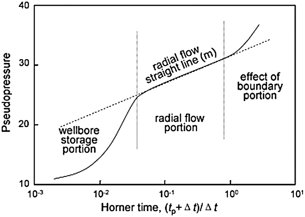
Figure 1: Semilog Horner plot for a pressure buildup test
Conventional RTA methods like Arps and Fetkovich methods did not account for the variations in operating conditions during the transient flow period, which is our main interest. Blasingame et al. accounted for changing operating conditions by defining a function called the superposition time function, also referred to as the material balance time. Blasingame et al. introduced two other functions to further smooth the data and get a unique match on the type curves; these two functions are rate integral function and rate-integral derivative function. The Material Balance Time Function could normalize any rate or pressure history so that it can account for the production conditions variations [13–21].
2.1 Material Balance Time Theory
The concept of material balance time is simply the time corrected relative to the cumulative production as per Eq. (3):
From Eq. (3), the functionality of the material balance time to normalize any rate or pressure history can be seen. Blasingame type curves are divided into three functions (Normalized rate, rate integral, and rate integral derivatives); each of them is plotted against the Material Balance Time.
It is simply defined as the rate divided by the flowing pressure drop as per Eq. (4):
It can be considered as the cumulative average of the rate at which the well was producing until a particular moment in time when plotted against the material balance time. It is considered as a method to remove the noise from the surface measured flowing rate and pressure, which helps in illustrating the reservoir signal. The integration removes any discontinuities in the raw data, resulting in a much smoother curve. This smooth curve is considered as a secondary curve match method in case we have any doubt in the Normalized Rate Type Curve. Eq. (5) illustrates the integration process:
It is the derivative of the rate integral function with respect to the material balance time as per Eq. (6):
After going through the different methods of drawing the type curves to get a unique match for our data set, in the next section, we are going to show how to calculate the parameters of skin and permeability after getting the sought match.
The daily production data was used in this study to get more resolution in the transient-part section. We could use any type of curve to calculate the parameters, but as mentioned earlier, the three curves are for clarity to help in getting the unique solution. The reservoir parameters can be calculated as Eqs. (7)–(10):
We performed PTA and RTA for three wells and compared the results of both analyses. For PTA, we used build-up tests to analyze the middle time region (MTR) to extract the skin (S) and permeability (K) for each well using Horner Pseudo-Producing Time due to Multi-Rate production time using the last flow rate [13–15]. For RTA, we used Blasingame Type Curves because we are investigating the transient flow period. Conventional RTA methods like Arps and Fetkovich methods did not account for the variations in operating conditions during the transient flow period, which is our main interest. Blasingame et al. accounted for changing operating conditions by defining a function called the superposition time function, also referred to as the material balance time. Blasingame et al. introduced two other functions to further smooth the data and get a unique match on the type curves; these two functions are rate integral function and rate-integral derivative function. The Material Balance Time Function could normalize any rate or pressure history, so that it can account for the production conditions variations [16–25].
3.1 Pressure Transient Analysis for Reservoir “A”
We performed PTA for Well A#08 through drilling the well for exploring reservoir “A”. The well was subjected to a flow after flow test consisted of producing the well at a series of stabilized increasing flow rates in succession without a shut-in period. The memory gauges measured the BHFP at the sand-face. Production periods were lasting almost for 8 h, followed by a shut-in period lasting for 60 h.
During the test, the well produced 20 MMSCFD with only 40 psi of reduction in pressure, which indicates a considerably high value of permeability. We could extract the values of skin and permeability from Figs. 2A and 2B, we noticed that the value of slope between the MTR and Late Time Region (LTR) was four times which indicated two no-flow boundaries of equal distances from the well.
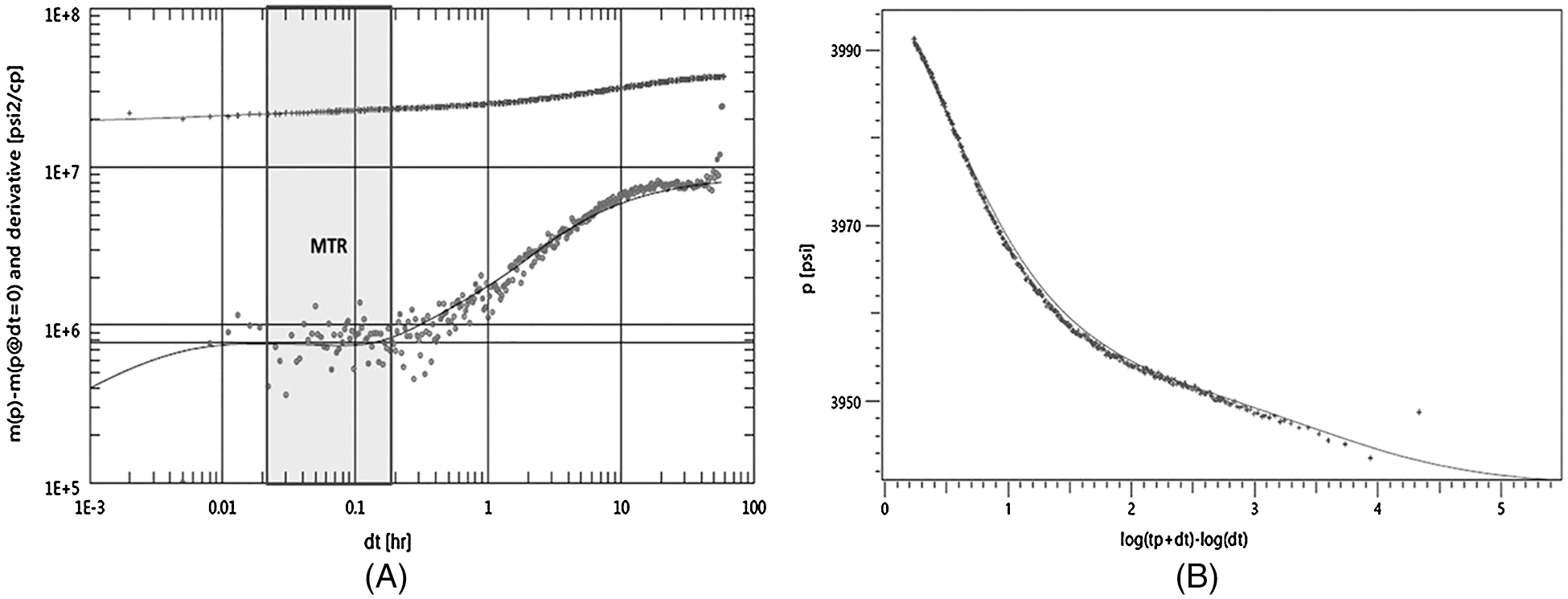
Figure 2: PTA of Well A#08, Test#01. (A) Log-Log Plot. (B) Horner plot
3.1.2 PTA for Well A#02, Test#02
We performed a flow after flow test in the same reservoir “A”. Each flow period was for 10 h, until the final build-up for 65 h. During the test, the well produced 5 MMSCFD with 145 psi of reduction in pressure, which indicated a lower permeability than the test before.
From Figs. 3A and 3B, we could extract the permeability and skin but we noticed that we did not reach any boundaries. That could lead us to believe that maybe the time of shut-in was not enough to feel the boundary due to the low permeability value. After contacting the exploration section, it was shown that the well was drilled in a channel.
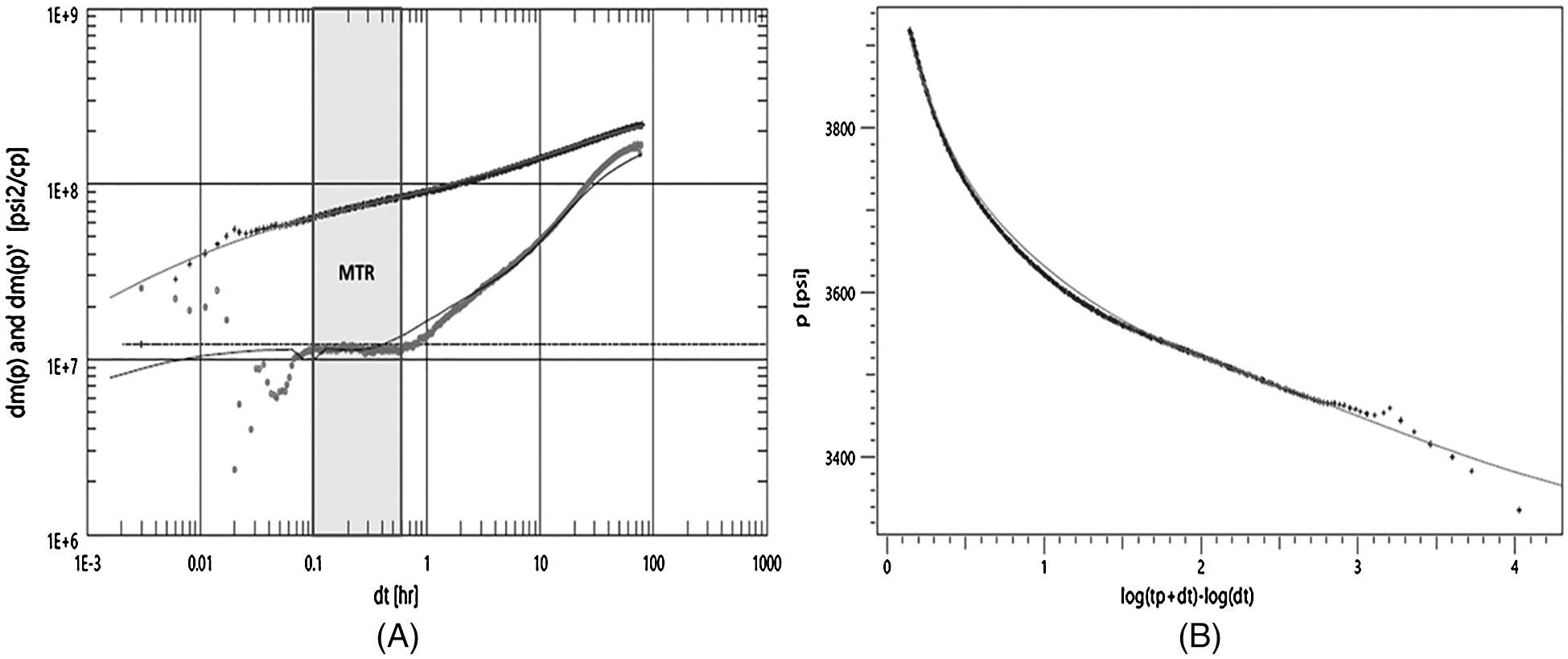
Figure 3: PTA of Well A#02, Test#02. (A) Log-Log plot. (B) Horner plot
The well was not producing as expected, so we performed PTA to only determine the skin and permeability to spot the problem. The flowing period was 12 h and the S/I period was 25 h. During the test, the well produced 1 MMSCFD with 1180 Pisa of reduction in pressure, which indicated a very low value of permeability.
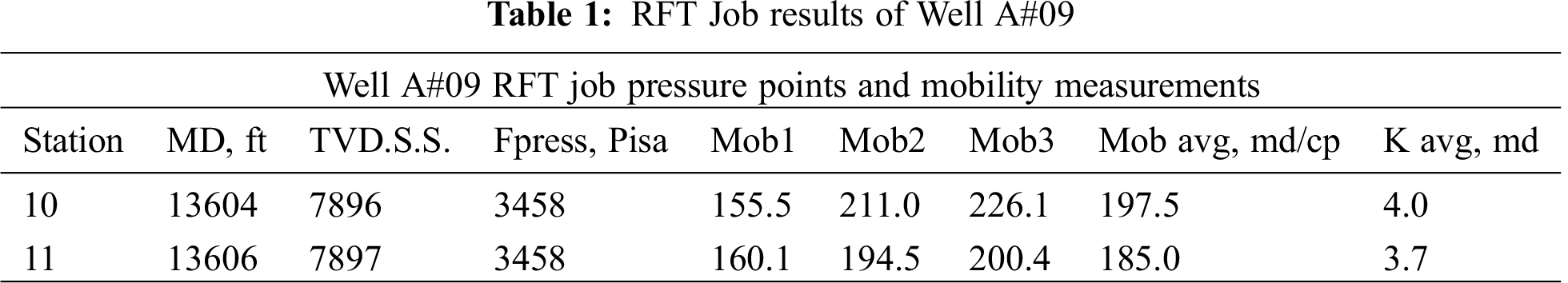
From Figs. 4A and 4B, we could extract the permeability and skin. From Fig. 4, we could see that we did not see the boundary-dominated flow because the main purpose of the test was mainly to determine the permeability and skin of this reservoir to investigate deeper into the reason for the low productivity of the well. Surface Read-Out (SRO) was used in the well but unfortunately, there was no way to close the well from below. We could see from Fig. 4A, in the early-time region (ETR), that we have the phenomena of changing wellbore storage; that happened because the well was shut-in from the surface not from below. The main reason for this phenomenon is phase redistribution [26–28]. We performed an RFT (Repeat Formation Tester) job, which gave us a qualitative indication of the permeability in the well during the drilling phase. The results are summarized in Tab. 1 [29–31].
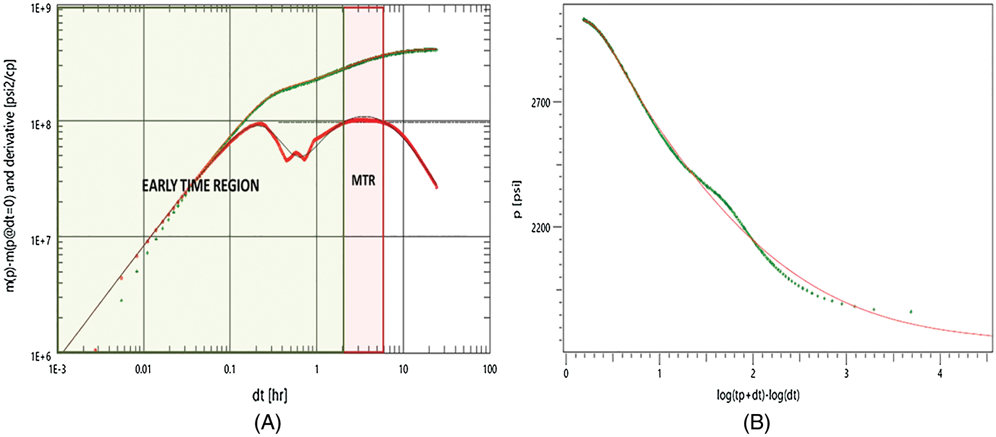
Figure 4: PTA of Well#09. (A) Log-Log plot. (B) Horner plot
3.2 Rate Transient Analysis for Reservoir “A”
We chose the stems that best match our data set; therefore, the reader may notice that for some figures one or two options of normalized rate, Integral or derivative were chosen. Depending on the clarity of the match, the interpreter may choose one, either two, or even three stems to get a more obvious match. The normalized rate for some data sets becomes scattered, so in these situations, it is preferred to go with Integral and derivative curves. The bottom hole flowing pressure is calculated using the Gray Correlation, which was developed by Gray, which was implemented into the software [32]. We used the daily production data of reservoir “A” from the multiphase flow meter in the production platform. The production data were reliable of third-party flow meter was used to check on the accuracy of the platform multiphase flowmeter for one whole year; After this period, the production operators kept on testing each well through the test separator every month to recalibrate the flow meter on the production platform.
The well was completed in Reservoir A and it was put into production in 2017 until now and the first production rate was about 19 MMSCFD on choke size 32/64”. From Fig. 5, we chose the stems that best match our data, we can notice that the well produced during the boundary-dominated flow. However, we could estimate the permeability and skin because we could confirm the stem selection using both the integral and derivative plots [33].
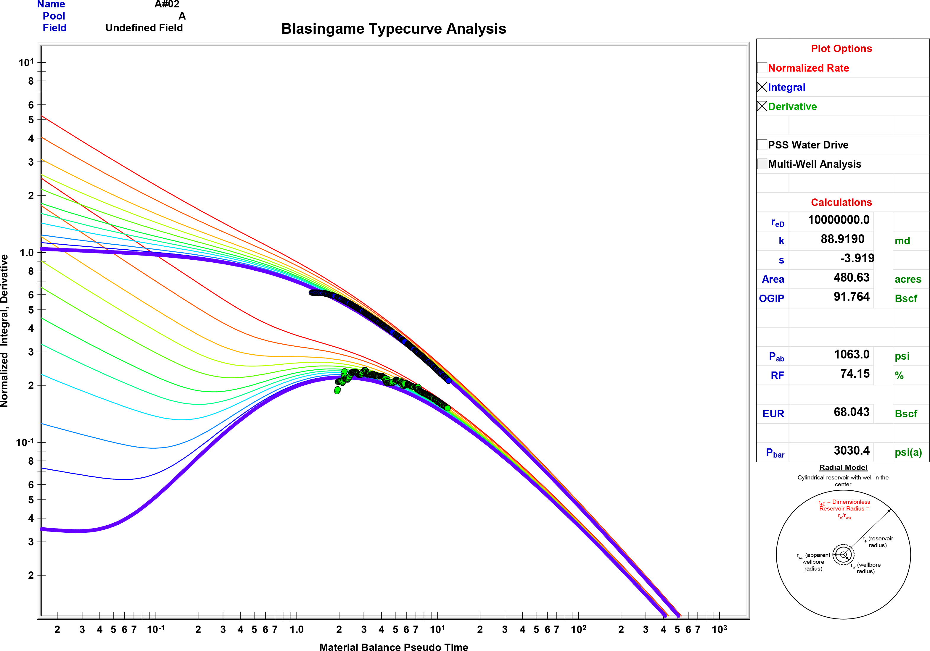
Figure 5: RTA of Well A#02, Blasingame type curve
The well was completed in Reservoir “A” and it was put into production in 2018 until now, and the first production rate was about 11.5 MMSCFD on choke size 32/64”. From Fig. 6, we chose the stems that best match our data, and we could see that the well was first produced during the pseudo-steady-state or transient-period until reaching the boundary dominated flow.
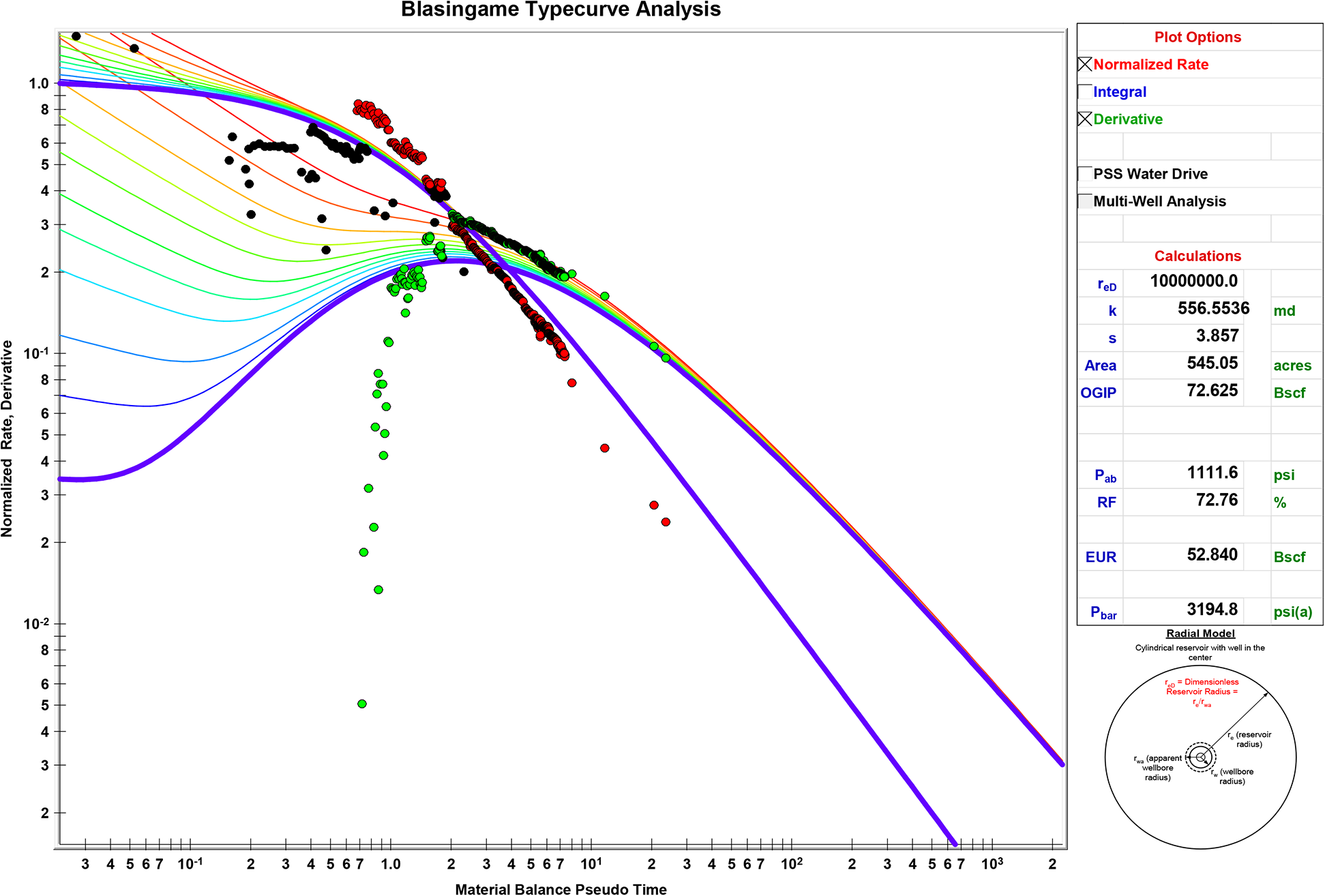
Figure 6: RTA of Well A#08, Blasingame type curve
The well was completed in Reservoir “A” and it was put into production in 2018 until now, and the first production rate was about 3.5 MMSCFD on choke size 32/64”. From Fig. 7, we chose the stems that best match our data and we could see that the well was first produced during the pseudo-steady-state or transient period until reaching the boundary-dominated flow.
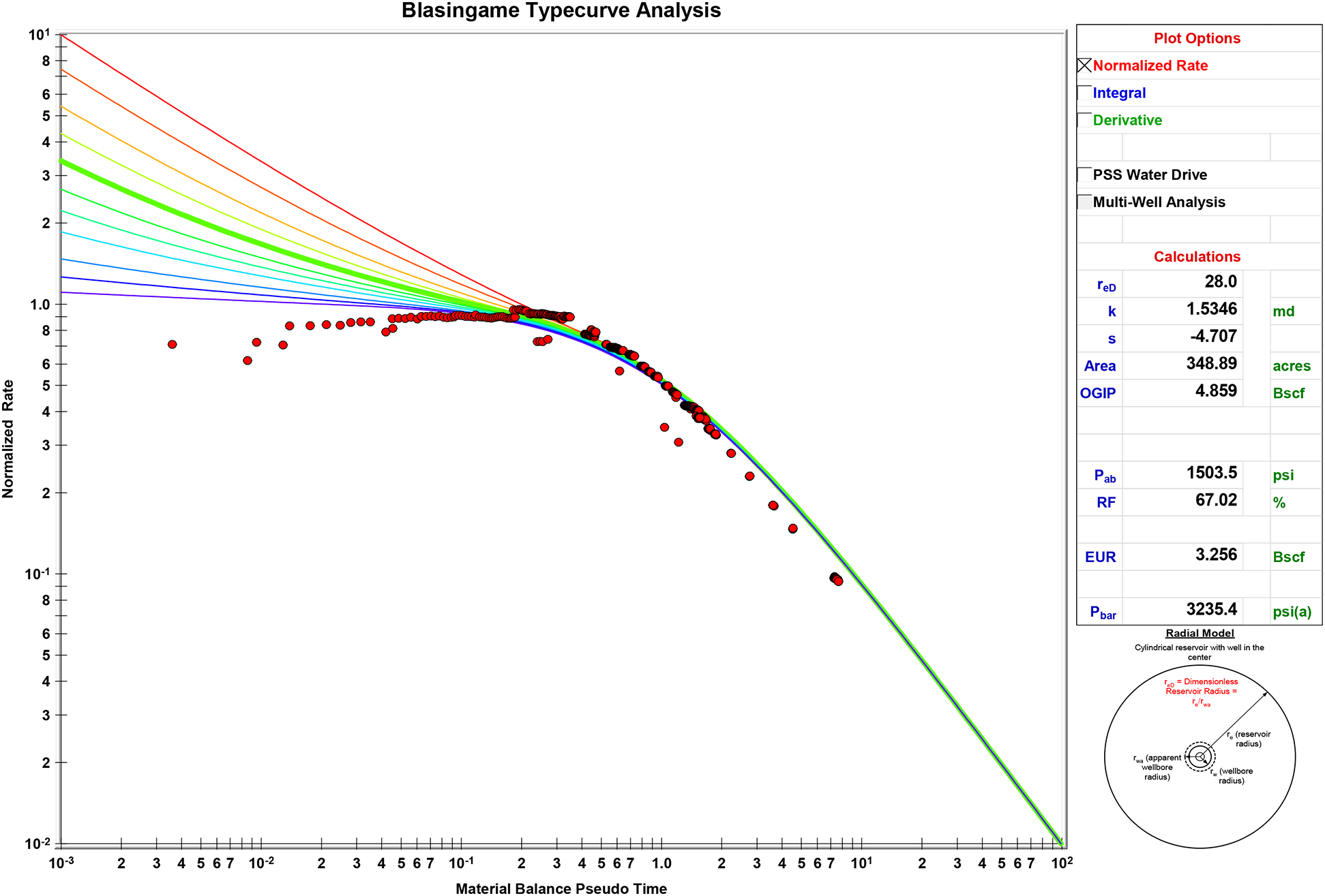
Figure 7: RTA of Well A#09, Blasingame type curve
Tab. 2 presents a comparison between the results of PTA and RTA. From Tab. 2, we could see that the results are almost similar between both analyses. Permeability values did not differ a lot between the two analyses; however, we did see a lower value of the skin in the RTA by a percentage of around 50% in Wells A#02 and A#08, because we performed the RTA after the completion of the wells while PTA was during the drilling phase (mud invasion damage is present). The difference in skin factor in Well A#09 is due to performing an acid job before performing RTA, as it was indicated earlier that the productivity of the well was not satisfying. The permeability variations showed that the reservoir is heterogeneous, and the three wells were at different locations in the reservoir as shown in Fig. 8. Despite that, we could get a match between PTA and RTA in the Gas Condensate Reservoirs for the first time while applying RTA for the three wells.
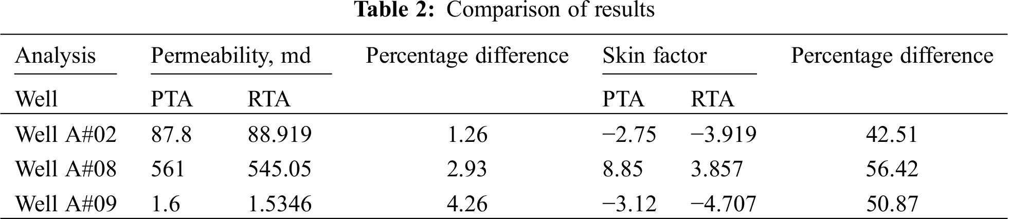
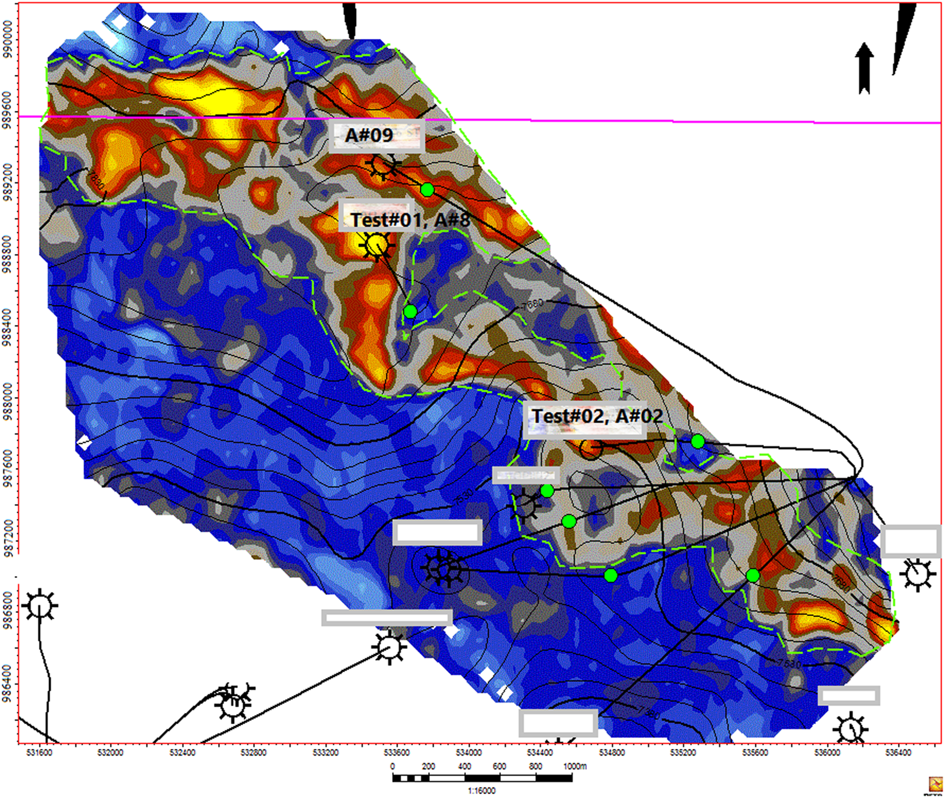
Figure 8: Structural Map showing Locations of the tested wells in reservoir (A)
We supposed that the high value of GOR (75,000 SCF/STB), would have a minimal effect on the RTA application in the Gas Condensate Reservoirs. Most of the recent researches applied the RTA in the Gas Reservoir, where the researchers used a compositional simulator to generate long-term production data over a wide range of the gas condensate reservoir parameters. In their studies, they tried to convert the parameters of gas condensate reservoirs (two-phase) to dry gas reservoirs (single-phase) to handle the multiphase flow problems using a reservoir compositional simulator [9]. In another recent research, the researchers used the single-phase type curves of Blasingame on gas condensate reservoirs, and they came up with the conclusion that condensate saturation would not have a severe effect on parameters estimates for high gas-oil ratio reservoirs, but they did not specify the value of the GOR. Therefore, they had to create an equivalent single-phase approach that came up with the right answers in Gas Condensate Reservoirs for low gas-oil ratio reservoirs [7].
We did not find any discrepancies between our study and the recent studies in the same field. However, we tried to set a reference value for the lowest GOR, below which we could not confirm the accuracy of applying RTA in Gas Condensate Reservoirs. We would suggest further research to investigate the lowest GOR, where we could apply the RTA and still get accurate results or matched results with the PTA. In our study, we used field data instead of synthetic generated production data to set the reference GOR.
The main objective of this study is to reduce the cost related to PTA by relying more on the RTA instead of PTA using Blasingame type curves to characterize the gas condensate reservoirs. Although the concept that Maximum Liquid Drop Out (MLDO) and GOR has a dominant effect on the application of RTA in Gas Condensate Reservoirs due to the condensate build up around the wellbore, which is stated in a lot of published literature. We found a great match between the RTA and PTA results after investigating wells with low MLDO of 3.14% and high gas-oil ratios of 75,000 SCF/STB. The results showed that despite the heterogeneity of the reservoir and the different locations of the three wells, the RTA could match the PTA results to a great extent. The following points are the main conclusion for the study for those who intend to use RTA as an alternative for PTA:
• The results obtained from the RTA in Gas Condensate Reservoirs are reliable as long as the GOR is 75,000 SCF/STB or higher and the MLDO is 3.14% or lower.
• GOR has a dominant effect on the application of RTA in Gas Condensate Reservoirs due to the condensate build-up around the wellbore in wells with high MLDO and low GOR.
• An accurate Multi-Phase flow meter is a great help to determine the flow rate for the two-phase flow condition.
• Using Downhole gauges is essential to obtain accurate results of the downhole pressure readings.
Although the results of permeability and skin factor were matched during the transient flow period; the OGIP (original gas in place) will be explored in future work during boundary-dominated flow.
Funding Statement: The authors received no specific funding for this work.
Conflicts of Interest: The authors declare that they have no conflicts of interest to report regarding the present study.
1. Johnson, C., Jamiolahmady, M. (2018). Production data analysis in gas condensate reservoirs using type curves and the equivalent single phase approach. Journal of Petroleum Science and Engineering, 171, 592–604. DOI 10.1016/j.petrol.2018.07.064. [Google Scholar] [CrossRef]
2. Agarwal, R. G., Gardner, D. C., Kleinsteiber, S. W., Fussell, D. D. (1999). Analyzing well production data using combined-type-curve and decline-curve analysis concepts. SPE Reservoir Evaluation & Engineering, 2, 478–486. DOI 10.2118/57916-PA. [Google Scholar] [CrossRef]
3. Al-Hussainy, R., Ramey, H. J., Crawford, P. (1966). The flow of real gases through porous media. Journal of Petroleum Technology, 18(5), 624–636. DOI 10.2118/1243-A-PA. [Google Scholar] [CrossRef]
4. Arps, J. (1945). Analysis of decline curve. Transactions of the AIME, 160(1), 228–247. DOI 10.2118/945228-G. [Google Scholar] [CrossRef]
5. Ayan, C., Hafez, H., Hurst, S., Kuchuk, F., O’Callaghan, A. et al. (2001). Characterizing permeability with formation testers. Oilfield Review, 13, 1–23. [Google Scholar]
6. Behmanesh, H., Hamdi, H., Clarkson, C. R. (2017). Production data analysis of gas condensate reservoirs using two-phase viscosity and two-phase compressibility. Journal of Natural Gas Science & Engineering, 47, 47–58. DOI 10.1016/j.jngse.2017.07.035. [Google Scholar] [CrossRef]
7. Blasingame, T., Johnston, J., Lee, W. (1989). Type-curve analysis using the pressure integral method. SPE California Regional Meeting. Bakersfield, CA. [Google Scholar]
8. Boogar, A., Gerami, S., Masihi, M. (2014). New modification on production data of Gas condensate reservoirs for rate transient analysis. Petroleum Science and Technology, 32(5), 543–554. DOI 10.1080/10916466.2010.506457. [Google Scholar] [CrossRef]
9. Bourdet, D. (2002). Well test analysis: The use of advanced interpretation models. Amsterdam: Elsevier Science. [Google Scholar]
10. CR, C. (2013). Production data analysis of unconventional gas wells: Review of theory and best practices. International Journal of Coal Geology, 109, 101–146. DOI 10.1016/j.coal.2013.01.002. [Google Scholar] [CrossRef]
11. Jensen, C., Mayson, H. (1985). Evaluation of permeabilities determined from repeat formation tester measurements made in the Prudhoe Bay Field. SPE Annual Technical Conference and Exhibition. Las Vegas, Nevada: Society of Petroleum Engineers. [Google Scholar]
12. Fekete User Help (2014) Http://Www.Fekete.Com/SAN/Theoryandequations.Html. [Google Scholar]
13. Fetkovich, M. (1980). Decline curve analysis using type curves. Journal of Petroleum Technology, 32(6), 1065–1077. DOI 10.2118/4629-PA. [Google Scholar] [CrossRef]
14. Fetkovich, M., Fetkovich, E., Fetkovich, M. (1996). Useful concepts for decline curve forecasting, reserve estimation, and analysis. SPE Reservoir Engineering, 11(1), 13–22. DOI 10.2118/28628-PA. [Google Scholar] [CrossRef]
15. Gray, H. (1978). Vertical flow correlation in gas wells. User’s manual for API 14B surface controlled subsurface safety valve sizing computer program. 2nd EditionDallas: American Petroleum Institute. [Google Scholar]
16. Hatzignatiou, D. G., Peres, A. M., Reynolds, A. (1994). Effect of wellbore storage on the analysis of multiphase flow pressure data. SPE Formation Evaluation, 9, 219–227. DOI 10.2118/19841-PA. [Google Scholar] [CrossRef]
17. Ilk, D., Anderson, D. M., Stotts, G. W., Mattar, L., Blasingame, T. (2010). Production data analysis_Challanges, pitfalls, diagnostics. SPE Annual Technical Conference and Exhibition, San Anotonio, Texas. [Google Scholar]
18. Islam, M. R., Muzemder, A. T., Khan, M. A., Hira, M. M. (2017). Rate transient analysis of well-07 and well-10 of habiganj gas field, Bangladesh. Journal of Petroleum Exploration and Production Technology, 7, 569–588. DOI 10.1007/s13202-016-0278-y. [Google Scholar] [CrossRef]
19. Lal, R. R. (2003). Well testing in Gas-condensate reservoirs (Master Thesis). Stanford: Stanford University. [Google Scholar]
20. Ezabadi, M., Ataei, A., Liang, T., Motaei, E., Othman, T. (2017). Production data analysis for reservoir characterization in conventional Gas fields: A new workflow and case study. SPE/IATMI Asia Pacific Oil & Gas Conference and Exhibition, Jakarta, Indonesia: Society of Petroleum Engineers. [Google Scholar]
21. Meunier, D., Stewart, G., Wittmann, M. J. (1985). Interpretation of pressure buildup test using in-situ measurement of afterflow. Journal of Petroleum Technology, 37(1), 143–152. DOI 10.2118/11463-PA. [Google Scholar] [CrossRef]
22. Nashawi, I. S., Elgibaly, A. A., Almehaideb, R. A. (1998). Pressure buildup analysis of gas wells with damage and non-darcy flow effect. Journal of Petroleum and Science Engineering, 21, 15–26. DOI 10.1016/S0920-4105(98)00043-6. [Google Scholar] [CrossRef]
23. Nashawi, I., Elgibaly, A., Almehaideb, R. (1998). Variable-Rate pressure-dRawdown analysis of gas wells with turbulence and damage. In Situ, 22(3), 291–320. [Google Scholar]
24. Okunola, D. (2008). Improving long-term production data analysis using pressure transient analysis techniques (Master Thesis). Texas: Texas A & M University. [Google Scholar]
25. Roussennac, B. (2001). Gas-condensate well test analysis (Master Thesis). Stanford: Stanford University. [Google Scholar]
26. Salem, A. (2016). Distorted pressure-buildup tests by phase redistribution–Changing wellbore storage effects. Journal of Environmental Science, Computer Science and Engineering Technology, 3(12), 10–26. [Google Scholar]
27. Spivey, J., Lee, W. (1999). Variable wellbore storage models for a dual-volume wellbore. SPE Annual Technical Conference and Exhibition. Houston, Texas: Society of Petroleum Engineers. DOI 10.2118/56615-MS. [Google Scholar] [CrossRef]
28. Sun, H. (2015). Advanced production decline analysis and application. Gulf Professional Publishing. DOI 10.1016/C2014-0-01693-0. [Google Scholar] [CrossRef]
29. Sureshjani, M. H., Azin, R., Osfouri, S., Gerami, S. (2016). Production data analysis in a gas-condensate field: methodology, challenges, and uncertainties. Iranian Journal of Chemistry and Chemical Engineering, 35(2), 113–127. DOI 10.30492/ijcce.2016.19381. [Google Scholar] [CrossRef]
30. Tantawy, M. A., Soliman, M. M., Agamia, A. H., Gawish, A. Y. (2015). Evaluation of Gas condensate reservoirs using production data and well test analysis–Abu Qir fields Mediterranean Sea (Master Thesis). Faculty of Petroleum and Mining Engineering, Suez University, Egypt. [Google Scholar]
31. Trina, M., Mercede, T. (2003). Characterization of gas condensate reservoir using pressure transient and production data-Santa Barbara Field. Monagas Venezuela, Texas: MSC Texas A&M University. [Google Scholar]
32. Wattenbarger, R. A., Ramey, H. J. (1968). Gas well testing with turbulence, damage and wellbore storage. Journal of Petroleum Technology, 20(8), 877–887. DOI 10.2118/1835-PA. [Google Scholar] [CrossRef]
33. Yildiz, T. (1989). Analytical studies of wireline formation testing and pressure losses across gravel packs. LSU Historical Dissertations and Theses. Louisiana State University. https://digitalcommons.lsu.edu/gradschool_disstheses/4893. [Google Scholar]
 | This work is licensed under a Creative Commons Attribution 4.0 International License, which permits unrestricted use, distribution, and reproduction in any medium, provided the original work is properly cited. |