Energy Engineering

DOI: 10.32604/EE.2021.014938

ARTICLE

FCS-MPC Strategy for PV Grid-Connected Inverter Based on MLD Model

Xiaojuan Lu and Qingbo Zhang*

Lanzhou Jiaotong University, Lanzhou, 730070, China
*Corresponding Author: Qingbo Zhang. Email: zqb17802970657@163.com
Received: 11 November 2020; Accepted: 04 March 2021

1  Introduction

With the increasing development of new energy sources such as photovoltaics, the research of power electronic devices has increasingly become the focus of attention. The inverter is effective for the photovoltaic grid-connected system, and its performance determines the power quality of the photovoltaic system fed into the grid. At present, the performance of the converter is mainly improved by studying new topological structures [1,2] and advanced control strategies [3,4]. However, the full-bridge inverter is widely used as a medium-sized photovoltaic grid-connected inverter, so the research on its modeling and control strategy is of great significance.

The averaging method has always been an important modeling method in the inverter modeling theory, interestingly, the state-space averaging method being representative [5,6]. However, the main difficulty in inverter circuit research includes its hybrid nature and poor understanding of the variation law of inverter switches acquired by using the averaging method.

The MLD model serves as a model used to describe the hybrid characteristics of hybrid systems. The modeling process can be proceeded by an overall differential equation obtained by the marriage of discrete events and continuous events. Discrete-time is introduced into the expression in the form of logical variables, which provides a more accurate approach for the mathematical description of the mixed system with linear and nonlinear simultaneously. Li et al. [7–10] establishes the MLD model of the inverter circuit for the hybrid characteristics of the inverter circuit, and studied the control method of the circuit based on the MLD model. Sheng et al. [11–15] uses deadbeat, sliding mode, and intelligent control method to control the inverter.

Model predictive control can fully consider the constraints and non-linear factors of the control object, which is suitable for processing multi-variable systems and achieves multiple control objectives at the same time by minimizing the value of the objective function. Therefore, model predictive control is suitable for the control of power electronic circuits. However, one of the main difficulties in applying the model predictive control to power electronic circuits is the mixed-integer quadratic programming (MIQP) [10,16].

Han et al. adopting the FCS-MPC control method makes full use of the discrete characteristics of power electronic circuits and considers every possible combination of switching states of electronic circuits. Moreover, selecting the switching state that minimizes the objective function value as the control of the electronic circuit can effectively avoid complex MIQP problems [17–19].

This article first analyzes the topology of the full-bridge direct inverter, and introduces logic variables to represent the switching state of the inverter, thereby obtaining the system evolution equation. The hybrid system language editing tool HYSDEL is used to describe the definition of system auxiliary variables and the evolution of the state, and the MLD model is generated. Based on the MLD model, having studied the finite control set model predictive control, we put our efforts into designing the output current full state observer and proposing the optimal objective function of the system from the perspective of control. It not only makes the control more accurate, effectively avoids the problem of mixed-integer quadratic programming, but also reduces the THD value of the inverter circuit output current, improves the power quality of the inverter into the grid, and ensures that the current output waveform and the grid voltage waveform have the same frequency and phase so that the system output can meet the grid connection requirements more quickly and accurately. Finally, a simulation was carried out through MATLAB/Simulink, and the simulation results proved the correctness of the model and the effectiveness of the control method.

2  Hybrid Logic Dynamic Modeling of Photovoltaic Inverter

2.1 MLD Model

The MLD model is a model used to describe the hybrid characteristics of the hybrid system. The modeling process introduces logical variables into the expressions to uniformly express the hybrid characteristics of the linear switching process [20]. This modeling method is more accurate for the mathematical description of the hybrid system with linear and nonlinear at the same time, which can be expressed as the following formula:

{x(t+1)=Ax(t)+B1u(t)+B2δ(t)+B3z(t)y(t)=Cx(t)+D1u(t)+D2δ(t)+D3z(t)E2δ(t)+E3z(t)≤E1u(t)+E4x(t)+E5 (1)

where, x(t) represents the system state quantity; u(t) represents the system input control variable; y(t) represents the system output variable; δ(t) represents the system auxiliary logic variable; z(t) represents the auxiliary continuous variable; A, B, C, D, E are constant-coefficient matrices.

The core of the MLD model embodies in the system analysis in a single model. State analysis would be proceeded by combining the physical conditions and related algebras in the state space of all regions in the system into the same model. By introducing appropriate auxiliary variables, we can control multiple variables of the system and process the optimization of system constraints.

2.2 MLD Dynamic Modeling of Photovoltaic Grid-Connected Inverter

The photovoltaic inverter studied in this paper as shown in Fig. 1 is a full-bridge direct inverter composed of four IGBTs. In the grid-connected part, the LC filter method of resistance and inductance is added. Compared with traditional power frequency inverter, the transformer link is omitted, which makes the inverter efficiency more efficient and saves costs. Therefore, this direct photovoltaic inverter method will gradually replace the traditional power frequency inverter method and gradually become a relatively common topology in photovoltaic grid-connected inverter circuits.

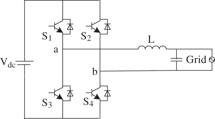
Figure 1: PV grid-connected inverter topological structure

In this circuit system, the input and output voltage can be regarded as a linear model, and the process of generating a voltage pulse sequence driven by the drive signal by the switch tube signal can be regarded as a typical nonlinear link. The voltage pulse signal acts on the circuit to make the circuit output continuous current. Therefore, photovoltaic grid-connected inverters constitute a typical hybrid system driven by discrete conditions and continuous state evolution.

Sn={1⇔Snon0⇔Snoff (2)

Set the first case: S1 and S4 are on, S2 and S3 are off, which is represented by λ = 1, namely:

λ=1↔S1=1,S4=1,S2=0,S3=0 (3)

Set S2 and S3 to be on, and S1 and S4 to be in another state when they are off, which is represented by λ = 0, namely:

λ=0↔S2=1,S3=1,S1=0,S4=0 (4)

By introducing the logic variable δ we can describe the direction of current ia. Setting the positive direction of current ia is shown in Fig. 1, and it is positive when flowing from the left side of the inductor to the right side. When iL > 0, it is represented by δ = 1, that is:

δ=1↔iL>0 (5)

When iL < 0, it is represented by δ = 0, namely:

δ=0↔iL<0 (6)

Therefore, according to the circuit topology, the logical relationship between the voltage uab and the inverter switch is obtained:

{uab=udc↔[λ=1,δ=1]∨[λ=1,δ=0]uab=−udc↔[λ=0,δ=1]∨[λ=0,δ=0] (7)

Bring it into the circuit topology to get:

{iL=Cducdt+igLdiLdt+riL+uc=uab (8)

According to the HYSDEL language, the corresponding MLD model difference equation is obtained by combining the logical relationship and the mixed characteristics:

{x˙=Ax+B1ig+B2uaby=Cx (9)

where, x=[iLuc] ; A=[ 0 1C−rL - 1L] ; B1=[−1C 0] ; B2=[01L] ; C=[0,1] .

Processing the obtained dynamic equations under the logical hybrid dynamic modeling, discretizing each parameter of the difference equation to obtain a new parameter equation:

{x(k+1)=A∗x(k)+B1∗ig(k)+B2∗uab(k)y=Cx(k) (10)

where, A∗=eAT ; B1∗=∫0TseATB1dt ; B2∗=∫0TseATB2dt .

3  Finite Control Set Model Predictive Control Strategy

The basic principle of FCS-MPC is to first perform online traversal calculations within the sampling period, according to the established system prediction model, to obtain the system output under the combination of each group of switches in the control set, and then establish an evaluation function for comparison, and finally select the order evaluation function. The switch function combined with the smallest value is used as the output signal to act on the inverter.

3.1 System Structure of Control Strategy

Fig. 2 is a block diagram of the FCS-MPC strategy. The application circuit is the single-phase photovoltaic inverter circuit topology with an output LC filter shown in Fig. 1. The important functions realized by the control block diagram in Fig. 2 are as follows:

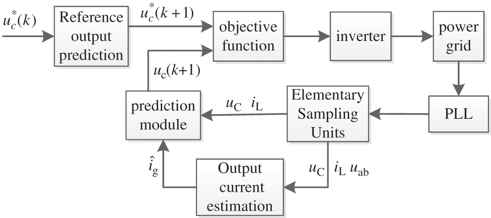
Figure 2: Block diagram of FCS-MPC

As shown in Fig. 3, we predict the reference the output voltage of the circuit at time k + 1 by referencing the output prediction module and input it to the objective function module. The prediction module predicts the output at k + 1 time by Eq. (9). The objective function module selects the optimal switching mode for circuit control according to the reference output and predicted output value of the circuit at k + 1. At each sampling moment, the grid voltage needs to be phase-locked so that the output after the system model is in the same frequency and phase as the grid voltage.

3.2 Reference Output Prediction Model

According to the basic principle of predictive control, the actual output of the system should follow the reference output as much as possible with the minimum amounts of errors. This article estimates the state of the system, and the reference voltage at k + 1 is solved by the following formula:

uc∗(k+1)=3uc∗(k−1)−2uc∗(k−2) (11)

3.3 Output Current Estimation

In order to use Eq. (10) to predict the output of the circuit, it is also necessary to know the output current ig of the circuit, but ig is usually inconvenient to measure. A simple method is to estimate the output current by measuring the filter current and output voltage, but estimation results are particularly sensitive to measurement noise because it is based on the derivative of the output voltage. Therefore, a full state observer is designed to estimate the output current ig.

{[x.i˙g]=[AB100][xig]+[B20]uaby=[C 0][xig](12)

Therefore, let [x ig]T be the state vector of the full state observer, then,

{[x^˙i^˙g]=[AB100][x^i^g]+[B20]uab+J(y−y^)y=[C 0][x^i^g] (13)

In the above formula, J is the observer coefficient; the superscript “^” represents the estimated value.

Thus, from Eq. (13), we can get:

[x^˙i^˙g]=Aobs[x^i^g]+[B20J][uabx^] (14)

where, Aobs=[AB100]−JC.

Thus, the estimated value of the output current can be obtained from the observer.

i^g=[0 0 1][x^i^g] (15)

It can be seen that the estimated value of the output current can be obtained from the filtered current iL and the output voltage uc and uab.

3.4 Selection of Objective Function

MPC predicts the state variables at the next moment through the current state variables and the switch state. The single-phase grid-connected inverter circuit studied in this paper has only 4 different switching modes. After the parameters are estimated at the future time, the optimization objective function is set. The objective function selected in this paper is:

g=(uc∗−uc)2+(ir−ig) (16)

where, uc is the actual output voltage, the reference output voltage is uc*, ir is the reference output current, and ig is the actual output current.

3.5 Control Process

The system samples the various parameters of the circuit at time k: uc is the grid voltage, the filter current is iL, the reference output voltage is uc*, and the output current is estimated, and then the objective function g is given the initial value g(i), and the output g(i)(i = 0, 1, 2, 3) of four different switching states was compared. The switch state S corresponding to the smallest g(i) is selected as the output of the control quantity at the next moment of the system.

4  Simulation and Experimental Verification

MATLAB/Simulink is used to simulate the FCS-MPC strategy based on the MLD model. The simulation parameters are as follows: Vdc = 400 V, filter inductance L = 100 ml, capacitance C = 1500 μF, rated frequency of 50 Hz.

The outputs in Fig. 4 are the predicted voltage and current waveforms of the switching function average model, and the outputs in Fig. 5 are the predicted voltage and current waveforms based on the MLD model. The connected load is a resistor-inductance load. It can be seen that, compared with Fig. 4, based on the predicted voltage and current of the mixed logic dynamic model in the first cycle, the voltage and current have stabilized, which can meet the grid connection requirements and have better dynamic characteristics. The estimated value of the output current observer and the actual value of the circuit is shown in Fig. 6. It can be seen that the observer can track the actual value of the circuit very well.

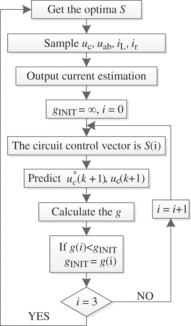
Figure 3: Flow chart of control

Figure 4: The predicted voltage and current waveforms based on switch function model

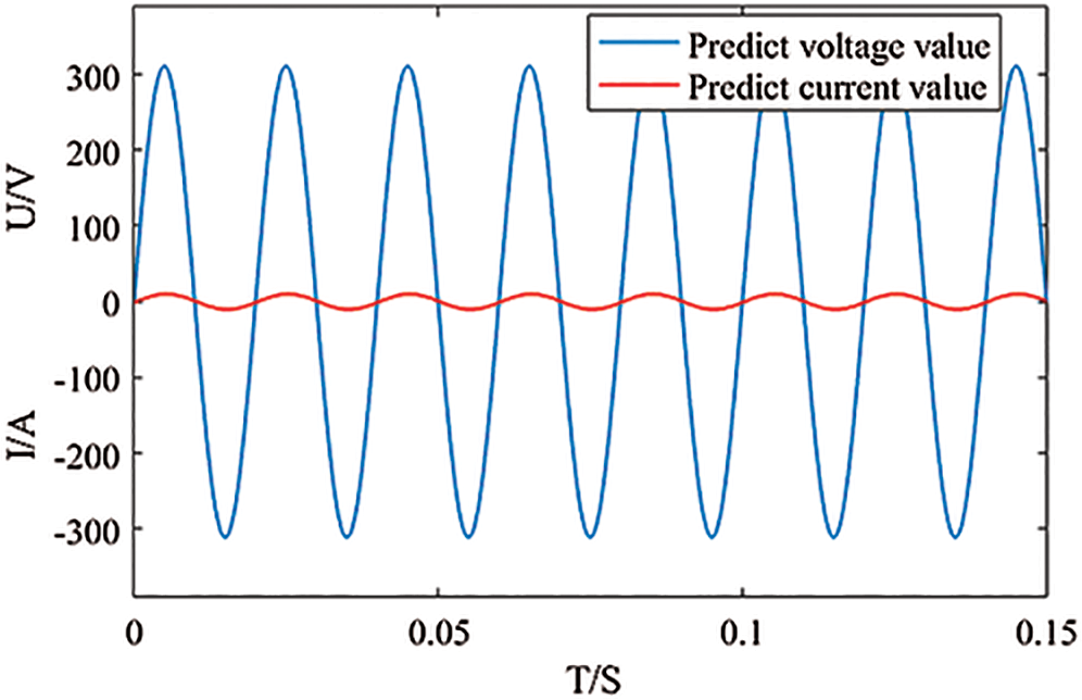
Figure 5: Predictive voltage and current waveform based on MLD model

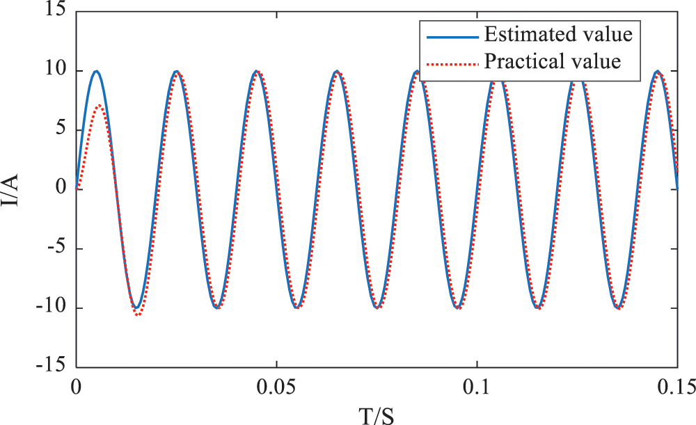
Figure 6: Comparison of estimated value of observer and practical value

The output voltage frequency of the designed system is shown in Fig. 7. It can be seen from Fig. 7 that during the simulation time, the minimum value of the system voltage output frequency is between 49.998 Hz and 49.999 Hz, and the maximum value is only between 50.006 Hz and 50.007 Hz. The frequency is maintained at 50 Hz, and the frequency of the grid voltage is also around 50 Hz. After modeling, the output voltage frequency can achieve the same frequency.

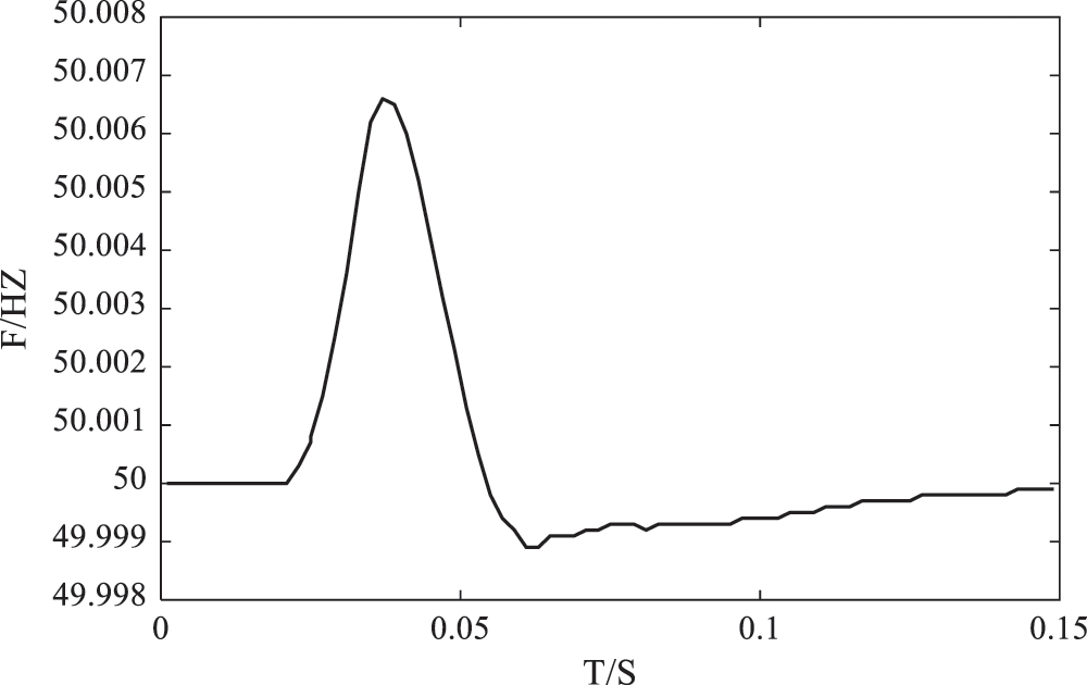
Figure 7: System grid output frequency diagram

The output inverter voltage and grid voltage, as well as the inverter voltage and grid current of the designed system, are shown in Figs. 8 and 9, respectively. It can be seen from the output waveform that the inverter voltage follows the grid voltage output. In the traditional switching function, it often takes several or more cycles to achieve the stable condition of the grid connection. In the logic hybrid dynamic modeling, the grid connection condition can be reached immediately, that is, the same frequency and phase, which can be better. To achieve the control effect, it is more effective.

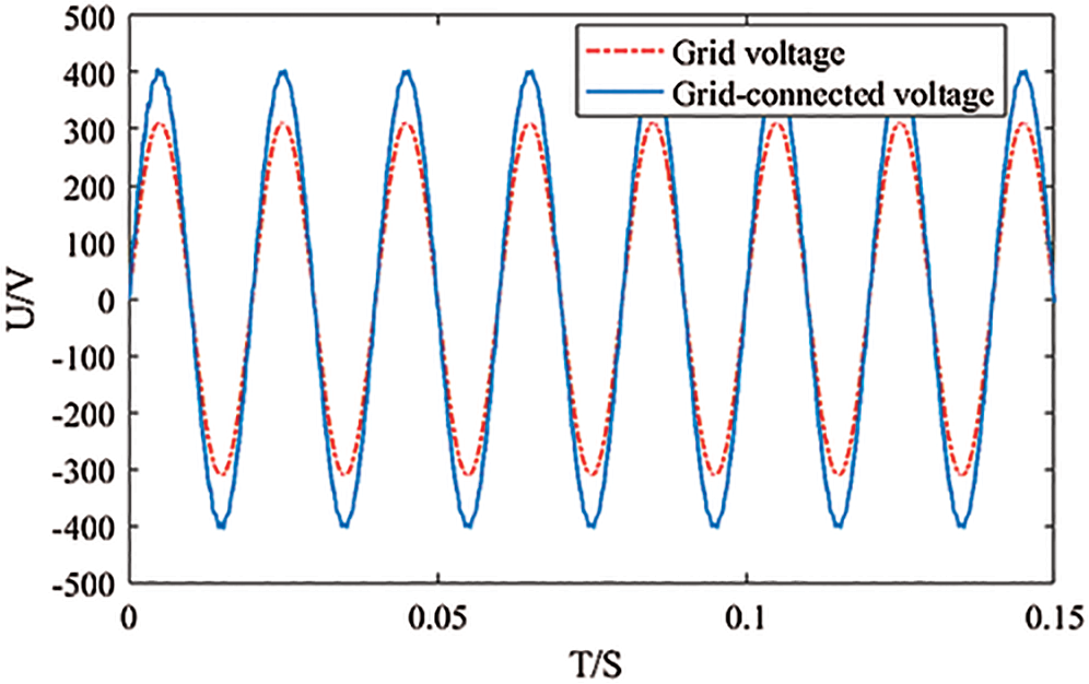
Figure 8: System grid output and grid-connected voltage waveform

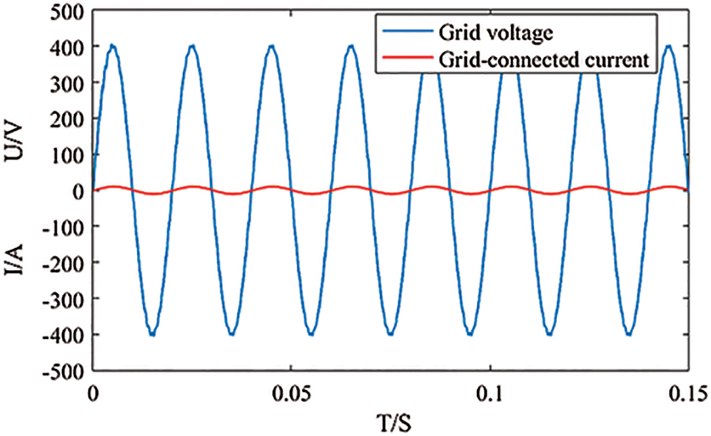
Figure 9: Grid output and grid-connected current waveform

Fig. 10 shows the comparison between the traditional switching function model and the MLD model proposed in this paper when the inverter works under different power conditions. According to the national standard GB/T 30427-2013 about the power factor of the grid-connected inverter, when the power factor of voltage and current can be stable above 0.99, it is selected as the grid-connected condition. The grid connection time of traditional switching function and MLD model are compared when the inverter works in the power range of 2 kW to 30 kW. It can be seen from the figure that the predictive control mode under the MLD model can meet the grid connection conditions faster.

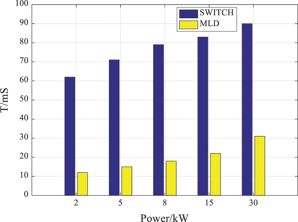
Figure 10: Comparison of grid-connection time of inverter with different power

From Figs. 11 and 12, the THD of the output current under the finite control set model predictive control strategy is 0.09%. The THD of the output current under the traditional model predictive control strategy is 2.82%. It can be seen that the quality of power input to the grid is improved under the finite control set model predictive control strategy.

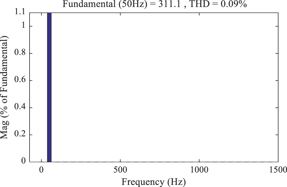
Figure 11: Current harmonic analysis of FCS-MPC control

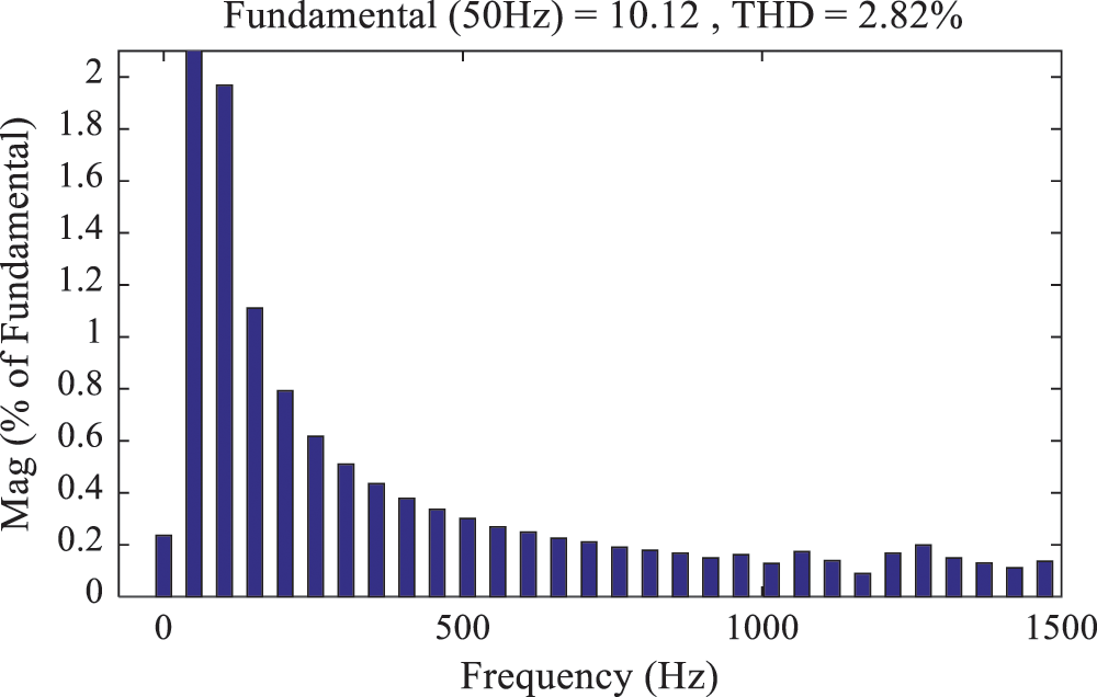
Figure 12: Current harmonic analysis of traditional model predictive control

5  Conclusions

This paper analyzes the MLD model of a single-phase photovoltaic grid-connected inverter circuit and uses it as a predictive model of the circuit. The FCS-MPC strategy is studied for a single-phase photovoltaic grid-connected inverter circuit with an output LC filter. The output current full state observer is designed, which not only effectively avoids the MIQP problem in the traditional predictive control, but also reduces the THD value of the inverter circuit output current, makes the grid-connected output voltage of the system have better power quality, and ensures the phase of the output waveform and the grid voltage waveform consistent so that the system output can meet the grid connection requirements more quickly and accurately. Simulation verified the feasibility and effectiveness of the control strategy.

Funding Statement: This paper is supported by the National Natural Science Foundation of China (Grant No. 51667013) and the Science and Technology Project of State Grid Corporation of China (Grant No. 52272219000 V).

Conflicts of Interest: The authors declare that they have no conflicts of interest to report regarding the present study.

This work is licensed under a Creative Commons Attribution 4.0 International License, which permits unrestricted use, distribution, and reproduction in any medium, provided the original work is properly cited.