| Energy Engineering |
DOI: 10.32604/EE.2021.014977
ARTICLE
Loss Analysis of Electromagnetic Linear Actuator Coupling Control Electromagnetic Mechanical System
1School of Transportation and Vehicle Engineering, Shandong University of Technology, Zibo, 255000, China
2School of Energy and Power, Jiangsu University of Science and Technology, Zhenjiang, 212000, China
*Corresponding Author: Cao Tan. Email: njusttancao@yeah.net
Received: 13 November 2020; Accepted: 18 March 2021
Abstract: As an energy converter, electromagnetic linear actuators (EMLAs) have been widely used in industries. Multidisciplinary methodology is a preferred tool for the design and optimization of EMLA. In this paper, a multidisciplinary method was proposed for revealing the influence mechanism of load on EMLA’s loss. The motion trajectory of EMLA is planned through tracking differentiator, an adaptive robust control was adopted to compensate the influence of load on motion trajectory. A control-electromagnetic-mechanical coupling model was established and verified experimentally. The influence laws of load change on EMLA’s loss, loss composition and loss distribution were analyzed quantitatively. The results show that the data error of experiment, and simulation result of input energy, mechanical work, and iron loss is less than 3%. The iron loss accounts for less than 54.9% of the total loss under no-load condition, while the iron loss increases with the increase of load. For iron loss distribution, only the percentage of inner yoke keeps increasing with the increase of load. The composition and distribution of loss are the basis of thermal analysis and design.
Keywords: Multidisciplinary methodology; electromagnetic linear actuator; loss analysis; control method; coupling model
As an energy converter, EMLAs have been widely used in industries because of their high power density, high linearity, and compact structure [1–3]. The EHLA based on linear actuator is becoming a research hotspot because of its good dynamic performance [4]. However, the large amount of heat generated by internal loss will lead to an undesirable temperature increase in EMLA [5–7]. There is an increasing demand for simultaneously solving related physical phenomena.
Currently, lumped parameter method [8], semi-analytical method [9], and numerical method [10–13] have been proposed for the thermal design and loss analysis of EMLA. The lumped parameter method is mainly employed for analysis of thermal resistance network as well as for calculation of conduction, convection, radiation, and contact thermal resistances for different components of actuators [14,15]. Lumped parameter method is characterized by low cost and faster calculation speed. For the finite element method (FEM), the heat conduction in a solid element with specific conductivity can be modeled, but the convection and radiation boundaries must be based on empirical correlations [16–18]. Loss analysis is the key to establish the accurate thermal model of EMLA and improve its working efficiency.
Typically, the static analysis method, quasi-static analysis method, and dynamic analysis method have been proposed for the loss analysis of EMLA. A thermal-electromagnetic coupled design methodology for linear actuators was proposed. The copper loss was considered as the source of temperature rise [19]. The influence of iron loss and mechanical loss on temperature rise was ignored in the static analysis method. In references [20,21], the iron loss and eddy current loss of the actuator using finite element analysis. The loss analysis was proposed under excitation current with a fixed mover. Although, the iron loss of the actuator at a certain position can be measured conveniently and accurately by the quasi-static loss analysis method [22]. The effect of loss by motion was neglected [23]. The iron loss with the fixed mover or unfixed mover was quantitatively analyzed and compared in [24]. The movement of the mover has a great influence on the electromagnetic field intensity and distribution. The accuracy of multidisciplinary methodologies which considering thermal and electromagnetic coupling with geometrical and temperature constraints can be improved by the dynamic analysis method [25]. Simultaneously solving related physical phenomena has become a necessary method. In the above works of literature, the influence of load on loss has not been researched.
To realize the application of the actuator, the motion curve must not change with the load. Therefore, the robustness of the control method and the tracking performance of EMLA need to be improved. Many compensations for disturbances have been proposed. Such as thermal disturbance, Coulomb friction, and other nonlinearities of the EMLA [26–28]. For systems with uncertain factors and variable disturbances, adaptive control is a good choice [29,30]. Compared with other nonlinear factors, the amplitude of load change is relatively large. It’s a challenge to design a trajectory tracking controller with variable load. The trajectory tracking controller is the basis of loss analysis considering load.
In this paper, a multidisciplinary method was proposed for revealing the influence mechanism of load on EMLA’s loss. The motion trajectory of EMLA is planned through tracking differentiator, an adaptive robust control was adopted to compensate the influence of load on motion trajectory. A control-electromagnetic-mechanical coupling model was established and verified experimentally. A coupling model including mechanical, electromagnetic, and control of EMLA is established in Section 2. Experimental verification is carried out and discussed in Section 3. The interaction between load and loss is analyzed quantitatively in Section 4. The work is concluded in Section 5.
2 Multidisciplinary Coupling Modelling
2.1 Electromagnetic-Mechanical Modelling
In this paper, a moving coil electromagnetic linear actuator is taken as an example to illustrate the multidisciplinary methodology, whose structure and principle are shown in [19] detail. The actuator has a cylindrically symmetrical configuration and consists of two sets of coils with opposite current, two yokes, a cover, a coil former, and a Halbach permanent magnet (PM) array, shown as Fig. 1. The actuator is a coupled electromagnetic-mechanical system, and the mathematic model can be described as
where u, i represent the input voltage and the current through the coil, respectively. R, L represent the resistance and inductance of the coil, respectively. ke, km represents the back electromotive force coefficient and the force sensitivity of the actuator respectively. Flf, Fld, Fd represent the electromagnet force, the load and the external disturbance respectively. m is the moving mass.
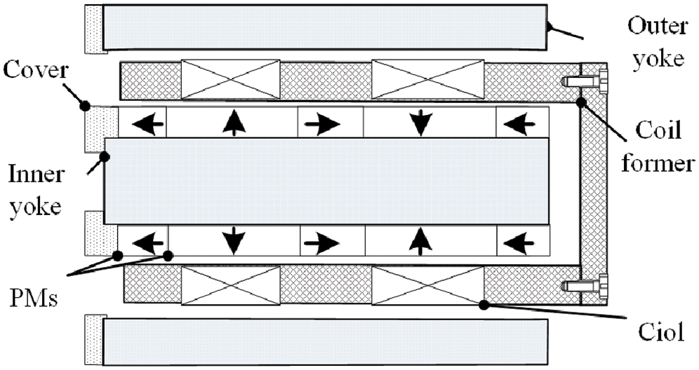
Figure 1: The schematic of bi-stable permanent magnet actuator
It can be perceived that EMLA’s losses mainly consist of copper loss and iron loss [24,27]. The copper loss ignoring the effect of temperature rise is expressed as
where R0 is the resistance measured at the base temperature. The iron loss, although difficult to approximate with the magnetic hysteresis and eddy currents are taken into account, whereas the stray loss is neglected, is calculated as
where Wiron is the iron loss volume density, B is the magnetic flux density, f is the excitation frequency, a and b are the empirical coefficient material related, kh and ked are the Steinmetz hysteresis loss coefficient and the eddy-current loss coefficient respectively. Under the influence of coil current, there is a strong eddy current along the circumferential direction at the inner yoke, because the inner yoke is not laminating the core structure (through thin sheets) or sintered powder metallurgy techniques [24].
2.3 Design of Trajectory Tracking Controller
The motion trajectory of the EMLA is planned through tracking differentiator (TD) [28]. In order to compensate the influence of variable load on the trajectory tracking control, an adaptive robust controller is proposed. The diagram of the adaptive robust control system is shown in Fig. 2. Since the inductance of the EMLA is small, it can be ignored for the simplified model. According to Eq. (1), a state-space can describe as follows:
where x1 = x, x2 = v denote the position and the velocity, respectively. The parameters are defined as θ = [θ1, θ2, θ3, θ4]T, where θ1 = mR/km, θ2 = ke, θ3 = RFld/km and θ4 is the nominal value of FdR/km,
where e = x1-xd is the tracking error,
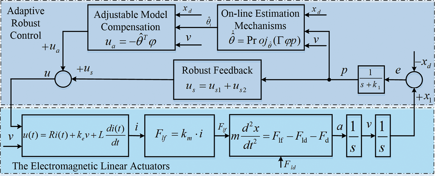
Figure 2: Diagram of adaptive robust control system
Eq. (6) is a transfer function with a steady convergence rate. By differentiating Eq. (4) and Eq. (5), the following equation can be obtained:
where
In order to compensate the major nonlinearities, including parameter variations and the external load variations. The following adaptive robust control is proposed
where ua is the model compensation term. us is a robust control law, in which us1 is used to stabilize the nominal system and us2 is a robust feedback term used to attenuate the effect of various model uncertainties.
In this study, FEM and analytical model were used to analyze the loss of EMLA considering the interactions among electromagnetic, mechanical, and control, shown as Fig. 3. 3D FEM modeling was realized with JMAG-Designer, while the mechanical and control modeling was realized with Matlab. The coupling model adopts the non-simplified 3D model. The 3D mesh model of EMLA is illustrated in Fig. 4. The material of the coil is copper, the material of the cover and yokes are steel, and NdFeB is used as the material of the permanent magnet. In order to ensure the strength of the coil carrier, PTEF is selected as its material. kh, ked, a, and b are materially related, which are set in the JMAG-Designer’s material library. In addition, the displacement and voltage of the coil were taken as the input for electromagnetic field calculation. The analysis results of the Lorentz force will be reversely coupled to adjust the displacement in the mechanical system. The analysis results of the armature reaction will be reversely coupled to adjust the voltage in the control system. All the above makes the coupling simulation more accurate and reliable.
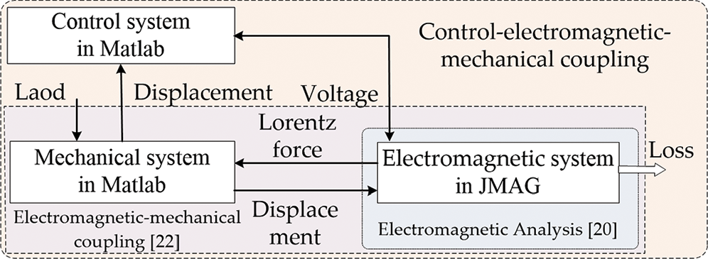
Figure 3: The control-electromagnetic-mechanical coupling model of EMLA
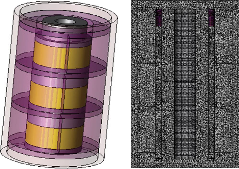
Figure 4: 3D model and mesh model of EMLA
A linear load simulator based on the moving coil electromagnetic linear actuator is developed, which could load the linear force accurately through the current control of the moving coil. The moving coils of EMLA and linear load simulator are designed with rigidity connections shown in Fig. 5. The linear load simulator is an electromagnetic linear actuator with the same parameters as the EMLA under force control [27]. The fixed-point Digital Signal Processor TMS320F2812 is chosen as the digital controller. The DSP control board, interface circuit, current sensors, and voltage sensor are integrated into the control unit.
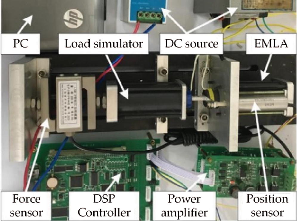
Figure 5: Experimental setup
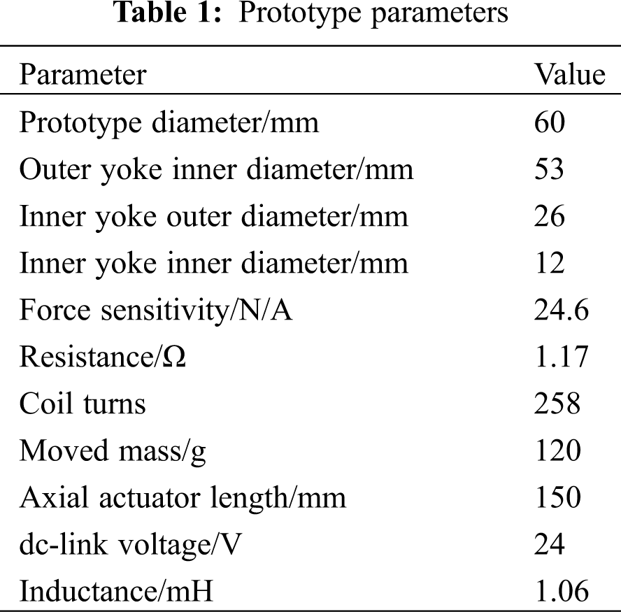
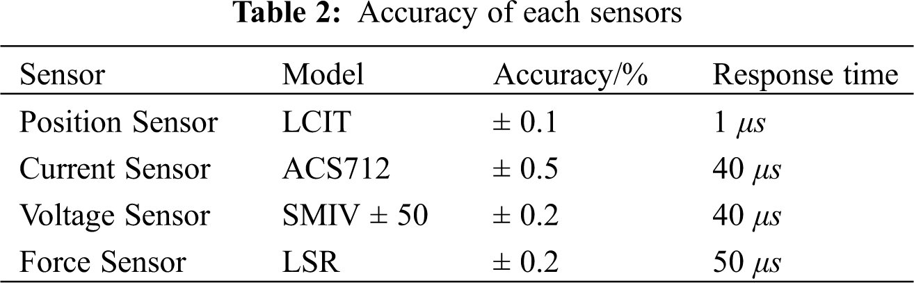
A force transducer is equipped to collect the force signals imposed on the stator of the linear load simulator according to Newton’s Third Law. Also, a position sensor is mounted by the side of EMLA to provide the position feedback, current sensors and voltage sensor are used to measure the input current and voltage of EMLA. The main parameter of EMLA is shown in Tab. 1 and the accuracy of each sensor is shown in Tab. 2.
To verify the effectiveness of the coupling model, the input energy (win) of actuator is obtained by integrating the product of coil current and coil voltage into time. The mechanical work done by electromagnetic force (wef) is converted into the negative work done by load and friction. In this paper, the friction of EMLA and linear load simulator was tested as the reference [27], which is shown in Fig. 6. The work done by friction is treated as a constant, due to the mover keeps the same motion curve. In every operation wf = 0.01 J, the working stroke is 10 mm. The work done by load is obtained by integrating the product of the load simulator output force and mover velocity into time. Thus, the iron loss is obtained indirectly in the test:
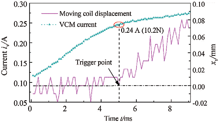
Figure 6: The friction of EMLA and linear load simulator
3.2 Experimental Setup Results
The load force output by load simulator is shown in Fig. 7, and the trajectory tracking result with different loads is shown in Fig. 8. The trigger time in Fig. 7 represents the time when the coil starts to move. The load simulator moves under the drive of the electromagnetic linear actuator, and the resulting back electromotive force makes the output load force smaller. The load force is adjusted to the target value after a certain period time under the action of the force control method. It can be seen from the figure that the load force varies within 3%.
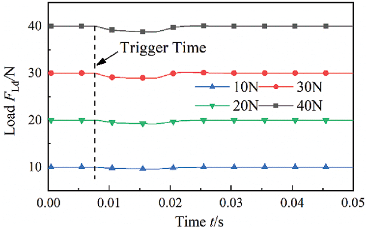
Figure 7: Load force output by load simulator
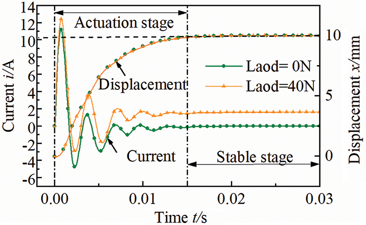
Figure 8: Trajectory tracking result with different load
The trajectory tracking curves coincide with different loads, under adaptive robust trajectory tracking control. This proves the effectiveness of the control method design. To further analyze the energy consumption of the EMLA, the working process of the EMLA is divided into two stages: actuation stage and stable stage. In the actuation stage, the mover moves from the initial position to the target position. The actuator needs to be applied with enough excitation current to drive mover moves to the target displacement, and the velocity is close to 0 when reaching the target displacement. In the stable stage, the mover stays firmly in the target position by the holding current. The holding current is determined by the load. The holding current is zero when the load is zero. Under the control system, the amplitude of current variation in the actuation stage and the holding current in the stable stage increase with the increase of load.
The experiment and simulation results of the power consumption vs. load are shown in Fig. 9. According to the error analysis, we can see that the accuracy of input energy (win), copper loss (wcopper), mechanical work (wef), and iron loss (wiron) are ± 0.7%, ± 1%, ± 0.2%, and ± 4.4%, respectively. The mechanical work which done by electromagnetic force, input energy, and copper loss increases linearly with the load. The increase of iron loss with load is relatively insignificant. Combining with the results in input energy, mechanical work, and iron loss, data error of experiment and simulation result is controlled within 3%. Which validates the correctness and precision of the control-electromagnetic-mechanical coupling model. The coupling model lays the foundation for the follow-up researches on quantitative analysis of loss, temperature inhibition, and multiphysics design of EMLA. However, the accuracy of the given results will be affected by various factors, in addition to the accuracy of the measurement equipment, the measurement noise will also affect it.
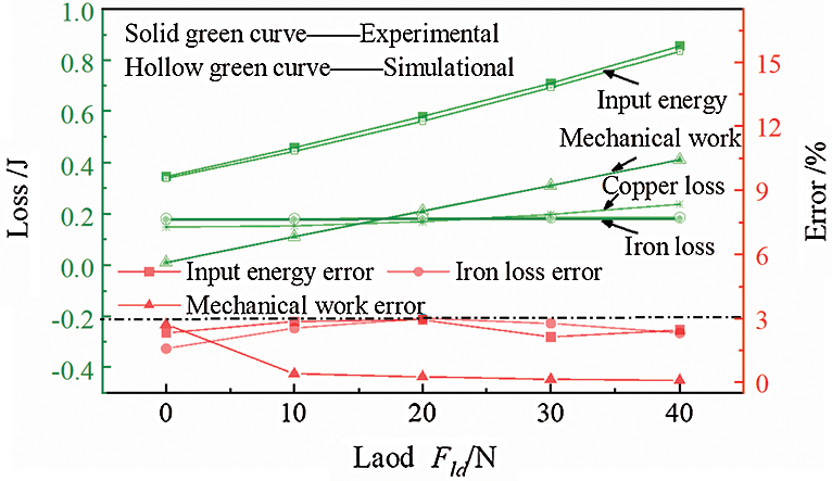
Figure 9: Experiment and simulation results of the power consumption vs. load
4 Quantitative Analysis and Discussion
4.1 Composition and Distribution of Loss without Load
In order to deeply analyze the composition and distribution of the loss, this paper quantitatively analyzes the loss of the EMLA in a single operation. Copper loss is produced by coil current, so the copper loss is concentrated in the coil. The inner yoke, outer yoke, cover, and permanent magnets all have a iron loss in the changing electromagnetic field. The iron loss includes hysteresis loss, eddy current loss, and stray loss. Because the EMLA is in the low-frequency working state, hysteresis loss and stray loss are very small, so the iron loss is mainly eddy loss. The cloud map of iron loss density of EMLA at peak value without load is shown in Fig. 10. The highest iron loss density point is located on the inner yoke close to the mover’s initial position, because the current rises rapidly at the beginning of the actuation stage, creating a strong eddy current. The inner yoke produces the highest average iron loss density in the whole working process. The inner yoke is inside the coil. Under the influence of coil current, there is a strong eddy current along the circumferential direction at the inner yoke, because the inner yoke is not laminating the core structure (through thin sheets) or sintered powder metallurgy techniques. Besides, the loss distribution of each element is an important basis for temperature calculation. The percentage of components’ loss in the total loss is shown in Fig. 11.
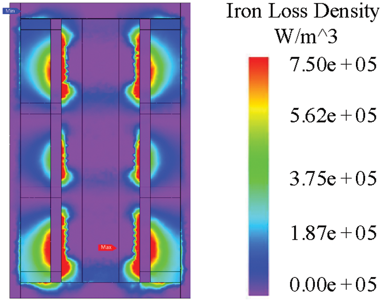
Figure 10: Cloud map of iron loss density of EMLA at peak value
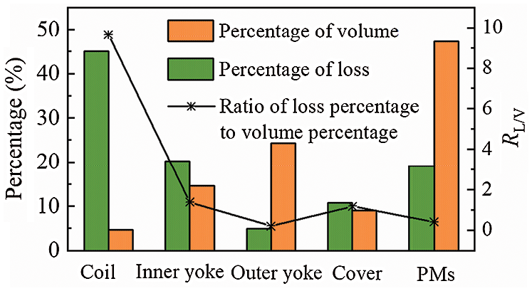
Figure 11: The volume percentage and loss percentage of each component
The loss in the stable stage is zero under no-load condition. Coil’s copper loss accounts for the highest proportion of the total loss, and coil’s loss accounts for 45.1% of the total loss. The ratio of loss from the largest to the smallest is the coil, inner yoke, PMs, cover, and outer yoke. PMs account for 47% of the total volume, due to the EMLA’s actuating force was maximized and linearized utilizing Halbach magnet array. The ratio of loss from the largest to the smallest is PMs, outer yoke, inner yoke, cover, and coil. RL/V is defined as the ratio of loss percentage to volume percentage. The RL/V of the coil is 9.0. The RL/V of the inner yoke and cover is less than 2. The RL/V of PMs and outer yoke are less than 1. Thus, the temperature rise of the coil locating inside the EMLA is obvious. At the same time, the temperature rise of the inner yoke locating inside the coil will be obvious, due to the closed space. Besides, the permissible temperature rising of PMs and coil is 180°C in the prototype. Therefore, the temperature rise of PMs and coil is an important index.
4.2 Impact of Load on Loss Composition
The change of load leads to the change of EMLA’s excitation current, which will cause the change of the actuator’s electromagnetic field. The results of EMLA’s loss versus load are shown in Fig. 12. The iron loss does not change with the load in the stable stage, and iron loss can be ignored. Copper loss and iron loss in the actuation stage increased by 33.2% and 2.8%, respectively, as the load increased from 0 to 40 N. Copper loss in the stable stage increased from 0 to 4.0 J, as the load increased from 0 to 40 N. The copper loss in the stable stage is generated by the holding current, which is proportional to the load. Since the displacement curve in the actuation stage remains unchanged, the EMLA needs to produce the same acceleration and deceleration, the excitation current changes with the load. As the copper loss is proportional to the square of the current, the copper loss of the EMLA increases rapidly with the increase of load. The increase of iron loss in the actuation stage is relatively slow, because the iron loss is related to the electromagnetic field strength and change frequency, and the electromagnetic field change frequency does not change when the load increases.
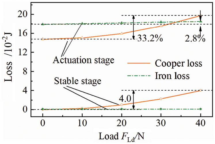
Figure 12: The results of EMLA's loss composition vs. load
The loss composition percentage in the actuation stage is shown in Fig. 13. The copper loss accounts for 45.1% of the total loss under no-load condition, while the iron loss accounts for 54.9% of the total loss. With the increase of load, the percentage of copper loss in the actuation stage increases gradually. The percentage of copper loss and iron loss in the actuation stage is the same when the load is 34 N. When the load is greater than 34 N, the percentage of copper loss is greater than that of iron loss. Copper loss increases rapidly in the stable stage, while the iron loss can be ignored, as the load increased. Therefore, the percentage of iron loss decreases with the increase of load, while the iron loss increases with the increase of load.
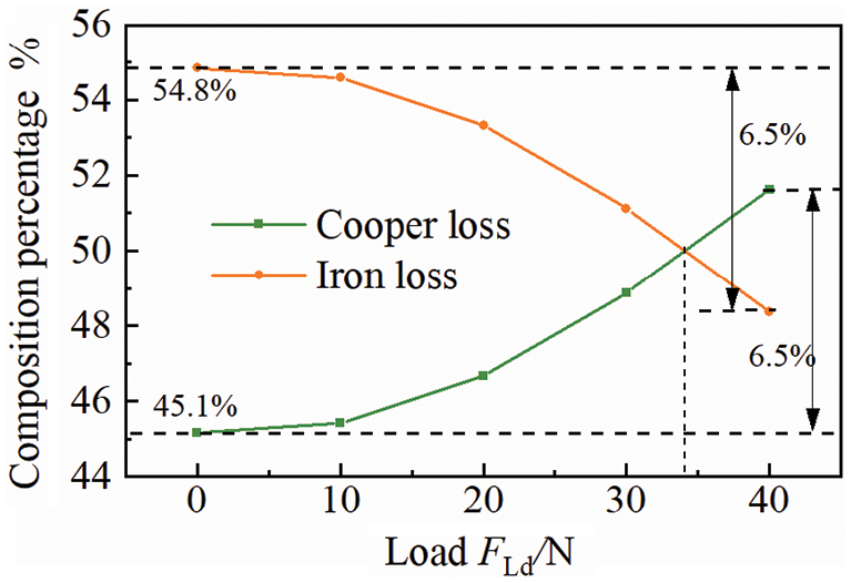
Figure 13: The loss composition percentage in actuation stage
4.3 Impact of Load on Loss Distribution
Since the copper loss is only distributed on coils, the iron loss distributes on the inner yoke, outer yoke, cover, and PMs with the load is mainly analyzed. The cloud map of iron loss density of EMLA at peak value with different load are shown in Fig. 14. The highest iron loss density point is located on the inner yoke close to the mover’s initial position, because the current rises rapidly at the beginning of the actuation stage, creating a strong eddy current. The average iron loss density of the actuator, from the largest to the smallest is the inner yoke, PMs, cover, and outer yoke. The loss distribution of each component does not change significantly with the increase of load. The area of high loss density area increases on the inner yoke and PMs. For quantitative analysis, the impact of load on loss distribution, the iron loss of each component with different load is shown in Fig. 15.
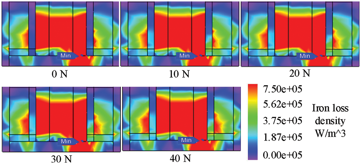
Figure 14: Cloud map of iron loss density of EMLA at peak value with different load
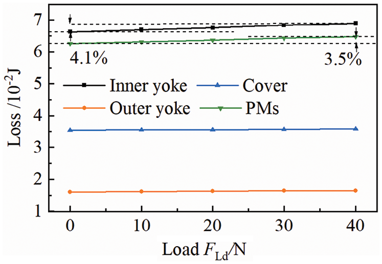
Figure 15: The iron loss of each component with different load
The iron loss on each component increases with the increase of load. The inner yoke’s iron loss and PMs’ iron loss increased by 4.1% and 3.5%, respectively, as the load increased from 0 to 40 N. While outer yoke’s iron loss and cover’s iron loss increased by 2.5% and 1.1%. The increase of inner yoke’s iron loss and PMs’ iron loss is less than outer yoke’s iron loss and cover’s iron loss. The changing amplitude of coil excitation current increases, the influence of coil armature reaction on the working magnetic field increases, as the load increased from 0 to 40 N. The magnetic field changes intensify on the inner yoke, PMs, and outer yoke, while has little influence on the cover.
The loss distribution percentage in each component with a different load is shown in Fig. 16. The iron loss of inner yoke and PMs always accounts for more than 70% of total iron loss. The percentage of inner yoke’s iron loss keeps increasing, while the percentage of cover’s iron loss keeps decreasing as the load increased from 0 to 40 N. The percentage of outer yoke’s iron loss and PMs’ iron loss is unaffected by the load. The impact of load on loss distribution lays a foundation for the research of loss reduction. Due to the EMLA’s actuating force was maximized and linearized utilizing Halbach magnet array. The change of PMs will significantly affect the performance of EMLA, so the study of the loss reduction should focus on the inner yoke and coils.
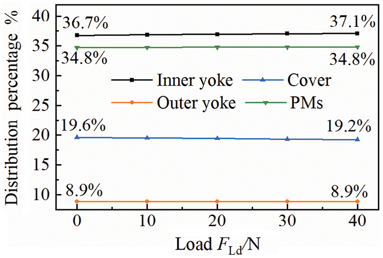
Figure 16: The loss distribution percentage in each component with different load
(1) The data error of experiment and simulation result of input energy, mechanical work, and iron loss is less than 3%. Which validates the correctness and precision of the control-electromagnetic-mechanical coupling model using the multidisciplinary methodology.
(2) The iron loss accounts for 54.9% of the total loss under no-load condition. The percentage of iron loss decreases, while the iron loss increases with the increase of load.
(3) The iron loss of inner yoke and PMs always accounts for more than 70% of total iron loss. Only the percentage of inner yoke’s iron loss keeps increasing with the increase of load.
Acknowledgement: This research was funded by the National Natural Science Foundation of China, Grant Nos. 51905319, 51975341, 51875326, the National Key Research and Development Project, China under Grant 2017YFB0102004, and the Shandong Provincial Natural Science Foundation, China under Grant ZR2019MEE049.
Funding Statement: The authors received no specific funding for this study.
Conflicts of Interest: The authors declare that they have no conflicts of interest to report regarding the present study.
1. Ling, Z. J., Zhao, W. X., Ji, J. H. (2020). Overview of high force density permanent magnet linear actuator and its key technology. Transactions of China Electrotechnical Society, 35, 108–121. DOI 10.19595/j.cnki.1000-6753.tces.190275. [Google Scholar] [CrossRef]
2. Pan, D. H., Li, L. Y., Wang, M. Y. (2018). Modeling and optimization of air-core monopole linear motor based on multi-physical fields. IEEE Transactions on Industrial Electronics, 65, 9814–9824. DOI 10.1109/TIE.41. [Google Scholar] [CrossRef]
3. Tan, C., Li, B., Ge, W. Q., Sun, B. B. (2018). Design and analysis of a bi-stable linear force actuator for directly-driven metering pump. Smart Materials and Structures, 27, 107001. DOI 10.1088/1361-665X/aadde2. [Google Scholar] [CrossRef]
4. Li, B., Liu, Y. T., Tan, C., Qin, Q. J., Lu, Y. T. (2020). Review on electro-hydrostatic actuator: System configurations, design methods and control technologies. International Journal of Mechatronics and Manufacturing Systems, 13(4), 323–346. DOI 10.1504/IJMMS.2020.112356. [Google Scholar] [CrossRef]
5. Qin, W., Fan, Y., Xu, H. Z., Lv, G., Fang, J. (2018). A linear induction maglev motor with hts traveling magnetic electromagnetic halbach array. Transactions of China Electrotechnical Society, 33, 41–48. DOI 10.19595/j.cnki.1000-6753.tces.L80762. [Google Scholar] [CrossRef]
6. Zhou, Y. C., Chang, S. Q., Li, B., Guo, T. J. (2018). Mechanical automatic transmission linear shift actuator displacement cascade control. Electric Machines and Control, 22, 1–7. DOI 10.15938/j.emc.2018.07.001. [Google Scholar] [CrossRef]
7. Ren, L. W., Ban, X. J., Wu, F., Huang, X. L. (2019). Fuzzy reinforcement learning control for two degree of freedom flight attitude simulator. Electric Machines and Control, 23, 127–134. DOI 10.15938/j.emc.2019.11.016. [Google Scholar] [CrossRef]
8. Bracikowski, N., Hecquet, M., Brochet, P., Shirinskii, S. V. (2012). Multiphysics modeling of a permanent magnet synchronous machine by using lumped models. IEEE Transactions on Industrial Electronics, 59, 2426–2437. DOI 10.1109/TIE.2011.2169640. [Google Scholar] [CrossRef]
9. Wang, Y., Ionel, D. M., Staton, D. (2015). Ultrafast steady-state multiphysics model for PM and synchronous reluctance machines. IEEE Transactions on Industry Applications, 51, 3639–3646. DOI 10.1109/TIA.2015.2420623. [Google Scholar] [CrossRef]
10. Simpson, N., Mellor, P. H., Wrobel, R., Iordanidis, G. (2012). Coupled thermal-electromagnetic design of a short-duty, high-specific force linear actuator. 6th IET International Conference on Power Electronics. Machines and Drives (PEMD 2012), pp. 1–6. Bristol. [Google Scholar]
11. Simpson, N., Wrobel, R., Mellor, P. H. (2014). A multi-physics design methodology applied to a high-force-density short-duty linear actuator. IEEE Transactions on Industry Applications, 52, 2919–2929. DOI 10.1109/TIA.2016.2541085. [Google Scholar] [CrossRef]
12. Vong, P. K., Rodger, D. (2003). Coupled electromagnetic-thermal modeling of electrical machines. IEEE Transactions on Magnetics, 39, 1614–1617. DOI 10.1109/TMAG.2003.810420. [Google Scholar] [CrossRef]
13. Marignetti, F., Delli Colli, V., Coia, Y. (2008). Design of axial flux pm synchronous machines through 3-D coupled electromagnetic thermal and fluid-dynamical finite-element analysis. IEEE Transactions on Industrial Electronics, 55, 3591–3601. DOI 10.1109/TIE.2008.2005017. [Google Scholar] [CrossRef]
14. Nategh, S. (2012). Thermal analysis of a PMaSRM using partial FEA and lumped parameter modeling. IEEE Transactions on Energy Conversion, 27, 477–488. DOI 10.1109/TEC.2012.2188295. [Google Scholar] [CrossRef]
15. Enomoto, Y., Kitamura, M., Iwasaki, N. (2014). Evaluation of efficiency and temperature rise of permanent magnet synchronous motor depending on magnetic properties. International Journal of Applied Electromagnetics and Mechanics, 45, 779–786. DOI 10.3233/JAE-141906. [Google Scholar] [CrossRef]
16. Li, W., Cao, J., Zhang, X. (2010). Electrothermal analysis of induction motor with compound cage rotor used for PHEV. IEEE Transactions on Industrial Electronics, 57, 660–668. DOI 10.1109/TIE.2009.2033088. [Google Scholar] [CrossRef]
17. Komeza, K., Lefik, M., López-Fernández, X. M. (2014). Calculations of heat transfer coefficient and equivalent thermal conductivity for induction motors thermal analysis. International Journal of Applied Electromagnetics and Mechanics, 46, 375–380. DOI 10.3233/JAE-141948. [Google Scholar] [CrossRef]
18. Jiang, W., Jahns, T. M. (2015). Coupled electromagnetic–thermal analysis of electric machines including transient operation based on finite-element techniques. IEEE Transactions on Industry Applications, 51, 1880–1889. DOI 10.1109/TIA.2014.2345955. [Google Scholar] [CrossRef]
19. Tan, C., Chang, S., Liu, L., Dai, J., Gu, C. (2016). Research on electromagnetic linear actuator with high driving force density and short time operation. Journal of Nanjing University of Science and Technology: Natural Science Edition, 40, 509–514. DOI 10.14177/j.cnki.32-1397n.2016.40.05.001. [Google Scholar] [CrossRef]
20. Utsuno, M., Takai, M., Mizuno, T., Yamada, H. (2002). Comparison of the losses of a moving-magnet type linear oscillatory actuator under two driving methods. IEEE Transactions on Magnetics, 38, 3300–3302. DOI 10.1109/TMAG.2002.802291. [Google Scholar] [CrossRef]
21. Dai, J. G., Chang, S. Q. (2014). Loss analysis of electromagnetic linear actuator. International Journal of Applied Electromagnetics and Mechanics, 46, 471–482. DOI 10.3233/JAE-141783. [Google Scholar] [CrossRef]
22. Lu, J., Chang, S. (2019). A trajectory planning-based energy-optimal method for an EMVT system. Computer Modeling in Engineering and Sciences, 118(1), 91–109. DOI 10.31614/cmes.2019.04190. [Google Scholar] [CrossRef]
23. Xiong, C., Wang, L. Y., Zheng, W. P., Yang, K. X., Qu, X. P. et al. (2012). Power loss analysis of two kinds of moving magnetic linear oscillating motors. Small & Special Electrical Machines, 40, 27–30. DOI 10.3969/j.issn.1004-7018.2012.03.008 [Google Scholar] [CrossRef]
24. Tan, C., Li, B., Liu, Y., Ge, W., Sun, B. (2019). Multiphysics methodology for thermal modelling and quantitative analysis of electromagnetic linear actuator. Smart Materials and Structures, 28, 087001. DOI 10.1088/1361-665X/ab2d39. [Google Scholar] [CrossRef]
25. Eckert, P. R., Flores Filho, A. F., Perondi, E., Ferri, J., Goltz, E. (2016). Design methodology of a dual-halbach array linear actuator with thermal-electromagnetic coupling. Sensors, 16(3), 360. DOI 10.3390/s16030360. [Google Scholar] [CrossRef]
26. Vese, I. C., Marignetti, F., Radulescu, M. M. (2009). Multiphysics approach to numerical modeling of a permanent-magnet tubular linear motor. IEEE Transactions on Industrial Electronics, 57, 320–326. DOI 10.1109/TIE.2009.2030206. [Google Scholar] [CrossRef]
27. Tan, C., Ge, W., Fan, X., Lu, J., Li, B. et al. (2019). Bi-stable actuator measurement method based on voice coil motor. Sensors and Actuators A: Physical, 285, 59–66. DOI 10.1016/j.sna.2018.10.003. [Google Scholar] [CrossRef]
28. Lu, J., Chang, S., Liu, L., Fan, X. (2018). Point-to-point motions control of an electromagnetic direct-drive gas valve. Journal of Mechanical Science and Technology, 32, 363–371. DOI 10.1007/s12206-017-1236-4. [Google Scholar] [CrossRef]
29. Liao, J., Chen, Z., Yao, B. (2017). Performance-oriented coordinated adaptive robust control for four-wheel independently driven skid steer mobile robot. IEEE Access, 5, 19048–19057. DOI 10.1109/Access.6287639. [Google Scholar] [CrossRef]
30. Chen, Z., Yao, B., Wang, Q. (2015). Synthesis-based adaptive robust control of linear motor driven stages with high-frequency dynamics: A case study. IEEE/ASME Transactions on Mechatronics, 20, 1482–1490. DOI 10.1109/TMECH.2014.2369454. [Google Scholar] [CrossRef]
 | This work is licensed under a Creative Commons Attribution 4.0 International License, which permits unrestricted use, distribution, and reproduction in any medium, provided the original work is properly cited. |