Energy Engineering

DOI: 10.32604/EE.2021.015542

ARTICLE

A Hybrid Model Based on Back-Propagation Neural Network and Optimized Support Vector Machine with Particle Swarm Algorithm for Assessing Blade Icing on Wind Turbines

Xiyang Li1,2, Bin Cheng1,2, Hui Zhang1,2,*, Xianghan Zhang1 and Zhi Yun1

1College of Mechanical and Electrical Engineering, Shihezi University, Shihezi, 832003, China
2Key Laboratory of Northwest Agricultural Equipment, Ministry of Agriculture and Rural Affairs, Shihezi, 832003, China
*Corresponding Author: Hui Zhang. Email: shzuzhanghui@163.com
Received: 26 December 2020; Accepted: 21 May 2021

1  Introduction

Wind energy is a type of green energy that can potentially replace fossil fuels and is currently being vigorously developed across the world. There are abundant wind resources on mountains, hills, valleys, lakes, and offshore areas. The cold and wet weather in high altitude and high elevation areas/regions are considered the main causes of icing on wind turbines. This problem of icing on turbine blades is often fatal and can be a serious safety hazard as well. The increase in loading and imbalance of wind turbine blades during normal operations because of icing, does not only affect the power output of the wind turbine, but may also easily lead to ice shedding due to the high-speed rotation of the blade, which potentially leads to safety related accidents [1–3]. These potential problems are the reason why it is important to properly analyze the icing of wind turbine blades.

At present, the diagnosis methods of wind turbine blade icing include blade icing detection system, ultrasonic method, numerical simulation method, state parameter method, data-driven method, etc., Skrimpas et al. [4–8] utilized an ice detection system or an external icing sensor to detect the icing state of the blades, However, the use of sensors to detect icing on wind turbine blades has detrimentally exhibited some problems that have resulted in increased costs of wind turbine manufacture, installation, operations, and replacement. At the same time, the installation of the sensor may change the aerodynamic performance of the blade, and with its continuous use under severe working conditions, the measurement error gradually increases and the accuracy decreases.

Muñoz et al. [9] adopted the ultrasonic method to accurately identify the icing state of the blade, but it cannot work normally when the weather condition is adverse. Villalpando et al. [10] used data analysis model to detect blade icing condition based on numerical mode and experimental mode, but there was no unified standard for the selection and calculation of parameters in the numerical simulation process, so it was difficult to ensure the accuracy of model analysis. Makkonen et al. [11] studied the sensitivity of the icing model to meteorological conditions, focusing on the study of the icing mechanism of wind turbine blades based on meteorological conditions, and compared the model prediction results with the ice cave icing test results. The validity of the model is confirmed. Dierer et al. [12–22] based on data mining and monitoring and control systems, a multivariate statistical method is used to build an intelligent model based on a large amount of data to detect and analyze the icing data of wind turbine blades to determine its icing status However, its model algorithm has higher requirements for feature screening. If effective feature screening cannot be performed, the accuracy of the overall algorithm is difficult to guarantee.

It is often practically convenient to assess and quantify the ice thickness by analyzing the changes in the environmental factors of icing on wind turbine blades. However, the operating environment of wind turbine blades is harsh, and many factors affect the icing process, such as temperature, humidity, wind speed, drop diameter, etc., which is a non-stationary random process. This requires icing prediction models of wind turbine blades to have strong generalization ability, accuracy, and stability. Based on outdoor natural environmental experiments, this paper established a mapping relationship between the environmental factors and wind turbine blade icing thickness. The environmental factors considered included temperature, humidity, wind speed, and droplet diameter. This paper innovatively proposes a hybrid model of PSO-SVM+BNPP for assessing and quantifying the icing on wind turbine blades accurately and as stable as possible. In the analysis, PSO was used to optimize the parameters of the SVM, while the PSO-SVM and the BPNN model were combined using dynamic weighting. This enabled the thickness of the wind turbine blade icing to be analyzed quickly, accurately, and steadily.

The rest of the paper is arranged as follows: Section 2–introduction of the single analysis method and the hybrid model used in the study. Section 3–data collection through experimentation and the establishment of the mapping relationship between multiple influencing factors and the degree of icing on the wind turbine blades. Section 4–utilization of the performance evaluation indicators to compare the performance of the models in icing on the wind turbine blades, and Section 5–further verification. And lastly, Section 6–the conclusion and recommendations.

2  Study Methodology

2.1 Particle Swarm Optimization (PSO)

PSO is an evolutionary computational algorithm. It is based on the concept that each particle can find the best local position according to its own flight process experienced in n-dimensional space. Moreover, the particle knows the best neighboring position, and its position and velocity are updated iteratively using the flight experience of its own history and that of the other particles’ [23–25].

The advantage of PSO is its simplicity and relative ease of implementation. Furthermore, it does not need many parametric adjustments to reach iterative convergence. The particles have only two attributes, namely: velocity (v) and position (pop), respectively. The positive and negative values of velocity represent the direction of their movements whilst all the values of position need to be absolute [26–28]. During analysis, each particle searches for the optimal solution individually in the search space and records it as the current individual extreme value (Pbest). Thereafter, it shares the individual extreme value with other particles in the entire swarm of particles. Lastly, it finds the best individual extreme value as the current global optimal solution (Gbest) for the entire swarm of particles [29]. Find the best learning factor c1 and c2 value through PSO , which is expressed in Eq. (1) thru to Eq. (4):

vi=vi+c1×rand×(Pbesti−popi)+c2×rand×(Gbest−popi) (1)

popi=popi+vi (2)

vi={vmin,vi,vmax,vi<vminvmin≤vi≤vmaxvi>vmax(1≤i≤a) (3)

popi={popmin,popi,popmax,popi<popminpopmin≤popi≤popmaxpopi>popmax(1≤i≤a) (4)

Eq. (1) is the velocity iteration formula. Eq. (2) is the iterative formula of the position. Eq. (3) and Eq. (4) defines the upper and lower limits for v and pop , which can prevent the model from overfitting. In the equations, vi is the current velocity, popi is the current particle position, the rand function generates random numbers between (0, 1), which is uniformly distributed, and c1 , are learning factors, and a is the number of iterations.

2.2 Support Vector Machines (SVM)

The ice thickness was analyzed and quantified using SVM. The learning factors, c1 and c2 , were obtained using the particle swarm algorithm corresponding to c (penalty factor) and g (parameter value in K function [kernel function]), respectively, in the support vector machine.

SVM is a type of a linear binary classifier defined in the feature space with maximum spacing, which differentiates it from a perceptron. It provides a solution by mapping the low-dimensional nonlinear space with the high-dimensional linear space through a kernel function k, which can be used to classify and analyze the nonlinear system [30–32]. The basic idea of SVM is to solve the training data set so that it can be correctly classified so that the maximum separation hyperplane can be obtained through geometric intervals [33].

When SVM is applied to a regression fitting analysis, the focus is no longer to find an optimal classification surface to separate the two types of samples, but instead to find an optimal classification surface to minimize the errors between all the training samples and the optimal classification surface [34].

Support Vector Machine for Regression (SVR) is a generalization of the Support Vector Classification (SVC). The hyperplane decision boundary in SVC is the threshold value used to assess the ice thickness of the wind turbine blades. The mathematical expression shown in Eq. (5):

fx=wTX+b=∑i=1naiyik(xi,xj)+b (5)

In Eq. (5), w is the normal vector of the hyperplane, b is the relative offset, and k is the kernel function expressed in Eq. (6):

k(xi,xj)=exp⁡(−g||xi−xj||2) (6)

Because the radial basis function has better performance in processing high-dimensional complex samples than other functions and requires fewer parameters, this paper chose the radial basis function as the kernel function. Thus, the used SVM regression function was obtained as expressed in Eq. (7) below:

f(x)=wϕ(x)+bminw,b⁡12||ω||2+c∑i=1nξi (7)

where ξ is the relaxation factor and c is the penalty factor.

2.3 Back-Propagation Neural Network (BPNN)

BPNN is a concept that was first proposed by Rumelhart and McClelland in 1986. It is a multi-layer feedforward neural network concept that is trained based on the error in the back-propagation algorithm [35,36]. The output results of the BPNN adopts forward propagation, while the error adopts the backward propagation. It emulates the activation and transmission like that of the human neurons. That is the input layer receives the data, while the output layer outputs the data [37]. The neurons of the first layer are connected to the neurons of the next layer where they collect the information transmitted by the neurons of the previous layer and pass the value to the next layer through an “activation” function [38]. BPNN has a strong nonlinear fitting ability and can map arbitrarily complex nonlinear relations. As shown in Fig. 1 the learning rules are simple, which is convenient for computer realization. The input data X are the environmental factors, mostly comprising of temperature, humidity, wind speed, and droplet diameter. The output data O is the ice thickness.

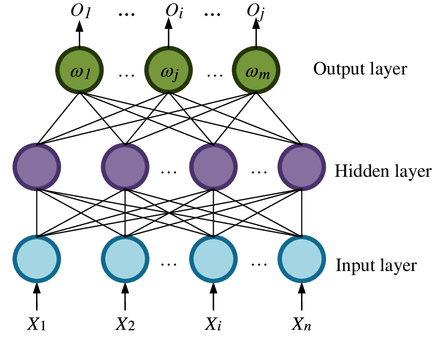
Figure 1: Structural diagram of the three-layer BPNN model

2.4 PSO-SVM+BPNN Model

By substituting the environmental factors of the training set such as temperature, humidity, wind speed, and droplet diameter into the PSO-SVM and BPNN models, the corresponding analytical results of the ice thickness for the training set are obtained. The ice thickness determined using PSO-SVM and BPNN is a weighted value and compared with the real ice thickness. By continuously adjusting the weight, the combined analytical results get close to the real icing thickness, The obtained weighting value “a” is thereafter used for the analysis [39]. On the basis of determining “a”, the next step is to fine tune the combined model in the same way. The disturbance parameters m and n are obtained, leading to an improvement in the analysis model. while retaining good generalization ability. It has a better ability to approximate the objective function and improve the accuracy of the diagnosis results. The combined formula for diagnosing the ice thickness Y is illustrated in Eq. (8):

Y=(a+m)y1+(1−a+n)y2 (8)

In Eq. (8), a is the weight, m and n are disturbances that are used for the optimization of the weight value. Parameter y1 is the diagnosis of icing thickness by the PSO-SVM model, and y2 is the diagnosis of icing thickness by the BNPP model. The Matlab software was used to simulate and actualize the solution of the icing thickness on the wind turbine blade.

2.5 Combination Diagnosis Model

First, normalize the data comprising of the meteorological environmental factors. Thereafter, the PSO-SVM and BPNN models are used for analysis. The diagnosis results are then weighted, and thereafter, a weight disturbance adjustment is performed, thus achieving weight optimization. Finally, the best diagnosis result is calculated, as shown in Fig. 2–ultimately generating the proposed hybrid diagnosis model.

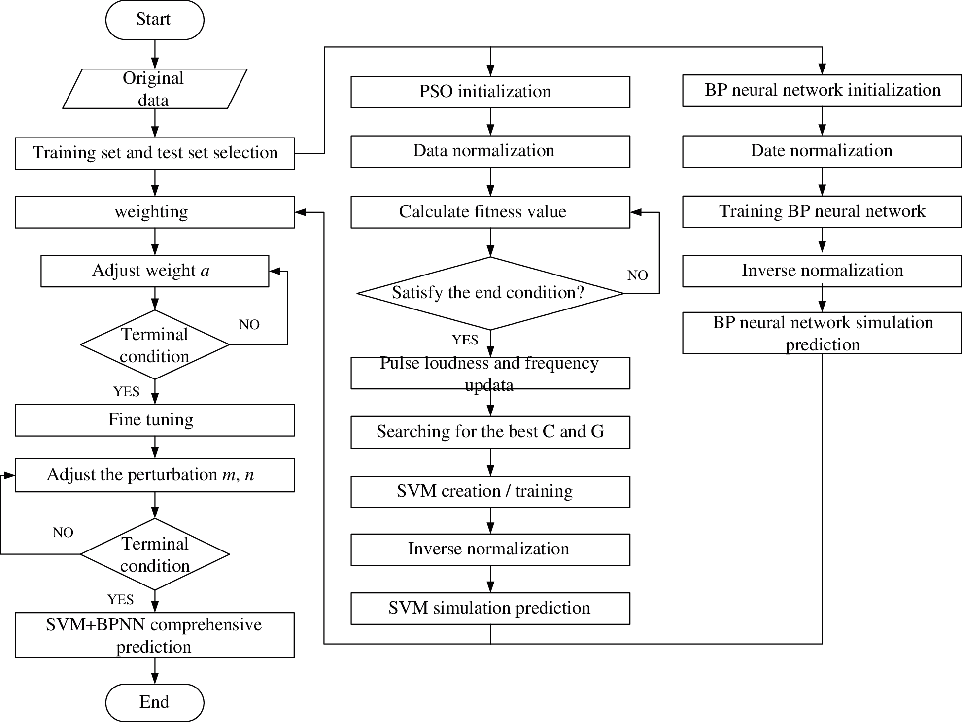
Figure 2: The combination diagnosis model of PSO-SVM+BNPP

3  Data Processing and Analysis

Factors affecting the icing of wind turbine blades are divided into external and internal factors. Internal factors consist of some of the physical characteristics of the wind turbine blades during the design process, including airfoil, material, and angle of attack. The external factors mainly include temperature, humidity, wind speed, and diameter of water drops. This paper studied the icing diagnosis on wind turbine blades from the perspective of external factors. Icing should meet the following three meteorological conditions, namely: (a) the wind speed should be in the range of 1 m/s～10 m/s, (b) the general air relative humidity should be more than 60%, and (c) the temperature should be below 0°C [40]. The icing process must satisfy the fluid law and the heat balance equation.

The test data for the study came from an ice coating test laboratory for rotating the wind turbine blade. The experimental setup is shown in Fig. 3. The airfoil of the wind turbine blade is NACA4412. The 1.5 MW wind turbine blade with 1:12.5 scale reduction was used as the test device, the length of blade wingspan R was 1.6 m, and the material of the blade shell is glass fiber reinforced epoxy resin. All the experimental data were collected with professional instruments that can be used to reflect the state changes during the icing process. The test was completed in a natural icing environment during winter. The test conditions were consistent with the actual environment of a local wind farm. The duration of the test period was 13 months. The wind speed adjustment used was 1380 type high-power industrial exhaust fan (138 cm * 138 cm) with a power of 1.1 kw, air volume of 45000 m3/h, an electricity voltage of 380 V, and an adjustable wind speed range of 0 to 20 m/s. The test used a high-pressure atomized water spray device to adjust the humidity of the test environment. The atomized water spray device is composed of: (a) a high-pressure water pump, and (b) three high-pressure water mist nozzles. The spray diameter of a single nozzle is 1 m. The pump power was 24 W. The change in the diameter of the water droplets was adjusted by rotating the nozzle to the desired orientation. The wind speed had a range of 2 m/s～6 m/s, the humidity range was 60%～85%, and the temperature range was −23°C～−10°C.

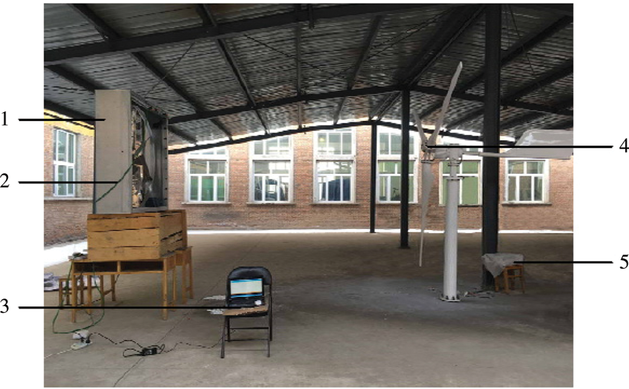
Figure 3: Icing test bench for wind power equipment. 1. Power input device fan, 2. Atomized water spray device, 3. Data collection device, 4. Wind generator, 5. Power storage box

During testing, the wind speed was measured by an AM-4201 digital anemometer. The temperature and humidity measurements were accomplished using a COS-03-X USB temperature and humidity recorder, respectively, which can record up to 2.08 million sets of data. The device is connected to a computer via a USB cable, and the data stored in the device can be imported into a desktop computer with the supporting software to facilitate subsequent data analysis. The ice thickness on the wind turbine blades was measured using an ultrasonic thickness gauge (with an accuracy of 0.1 mm) and a vernier caliper, with the data saved periodically as captured.

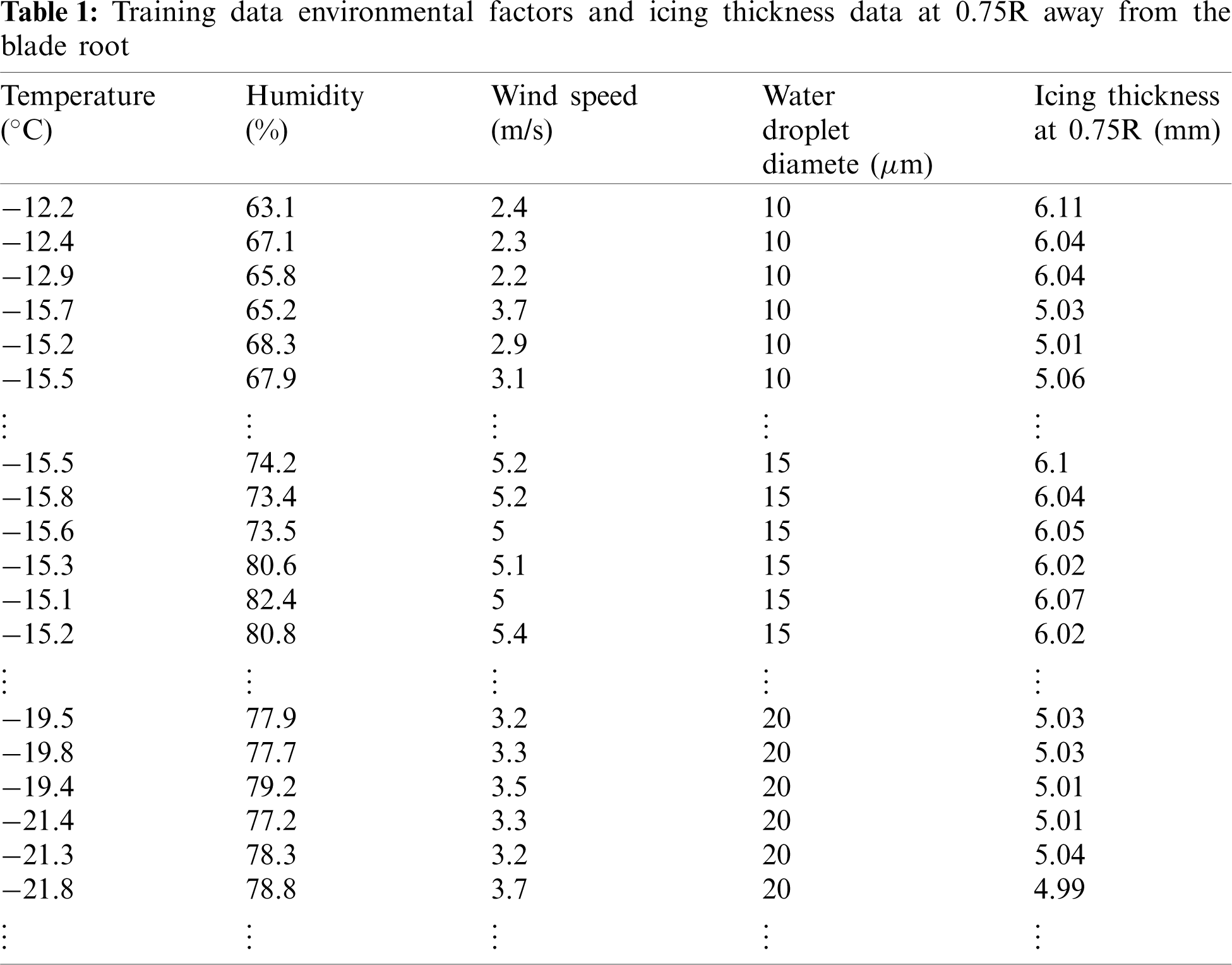
It was discovered through experimentation that the icing area increased with an increase in the wind speed. A droplet with a larger diameter forms larger ice crystal particles on the surface of the blade resulting in a rougher ice surface. With the decrease in temperature, the thickness of icing reduces. The reason for these changes is because the droplets in the air freeze directly into ice crystals alongside the decrease of temperature, resulting in a decreased number of liquid droplets impacting the surface of the wind turbine blades. When the humidity is low, the icing position is largely located at the outer leading edge of the blade. When the humidity is high, the icing position is mainly located at the leading edge and windward side, and thus, there is more icing. The front of the blade is the location for the most severe icing. Therefore, the icing thickness measurement point was selected at the blade front and 0.75R away from the blade root as shown in Fig. 4. The experimental data was obtained by conducting the test at 1 h interval. In total, 324 sets of data were collected at each measuring point, including the first 200 sets of data for training samples and the last 124 sets of data for test samples. The ice thickness data at 0.75R is shown in Fig. 5, with the corresponding environmental data shown in Fig. 6. The environmental data is shown in Tab. 1, As visually seen in the figures, there is no abnormality in the data or missing data points.

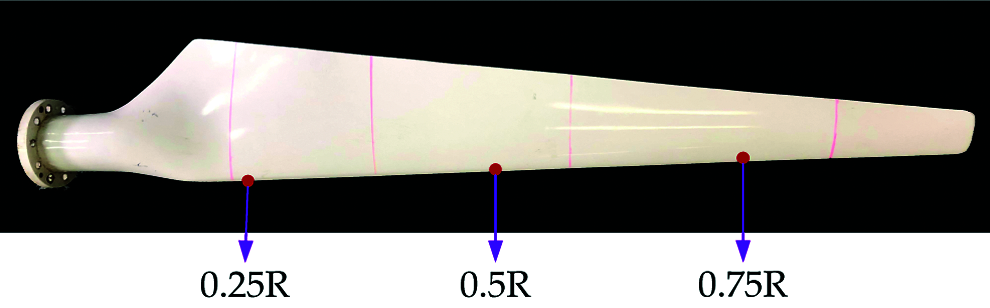
Figure 4: The wind turbine blade for icing experiment

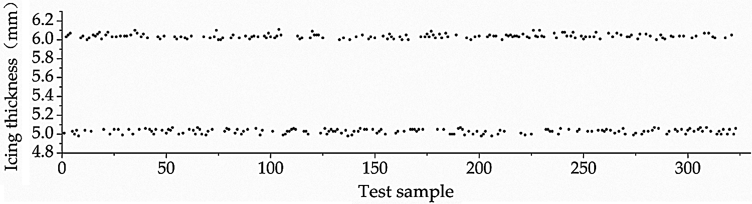
Figure 5: Icing thickness data at 0.75R away from the blade root

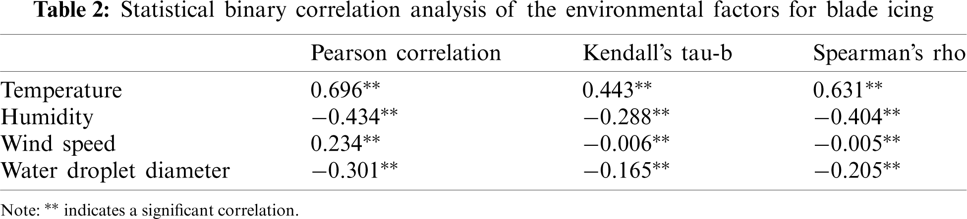
With the use of the SPASS software, Pearson correlation, Kendall's tau-b, and Spearman's Rho were used as the three evaluation indicators. Temperature, humidity, wind speed, water droplet diameter, and ice thickness were measured during the test and used for statistical binary correlation analysis. As shown in Tab. 2, environmental factors such as temperature, humidity, wind speed, and water droplet diameter all have an impact on the thickness of ice covering.

4  Case Studies

4.1 Performance Evaluation Index

To verify the performance of the model, Root Mean Squared Error (RMSE), Mean Absolute Deviation (MAD), and the coefficient of determination (R2) were used to compare the accuracy of all the models. The study measures the average diagnostic utility at each data point in the model. The statistical expressions used for the error computations and accuracy evaluation are shown in Eqs. (9)–(11):

RMSY=1n∑i=1n(xi−yi)2 (9)

MAD=1n∑i=1n|xi−yi| (10)

R2=1−∑i=1n(xi−x¯)2∑i=1n(xi−yi)2 (11)

Figure 6: Environmental factor data of blade icing: (a) Wind speed, (b) Humidity, (c) Temperature and (d) Droplet diameter

In Eq. (9) through to Eq. (11), n represents the number of test samples, xi represents the actual ice thickness, x¯ represents the average actual ice thickness, and yi represents the diagnosed ice thickness.

To verify the optimality of the model, this study compared the icing diagnosis of the wind turbine blade under different model settings. As shown in Fig. 6, the influencing factors and ice thickness were substituted into Parts 1 and 2 of the seven models. The hybrid diagnosis model comprising of PSO-SVM+BPNN was then compared with the MLR (Multiple Linear Regression), ELM (Extreme Learning Machine), SVM, BPNN, SVM+BPNN, and PSO-SVM model diagnosis results. The model accuracy was determined using the RMSE, MAD, and R2 parameters, respectively–see Eq. (9) through to Eq. (11) and Part 3 of Fig. 7.

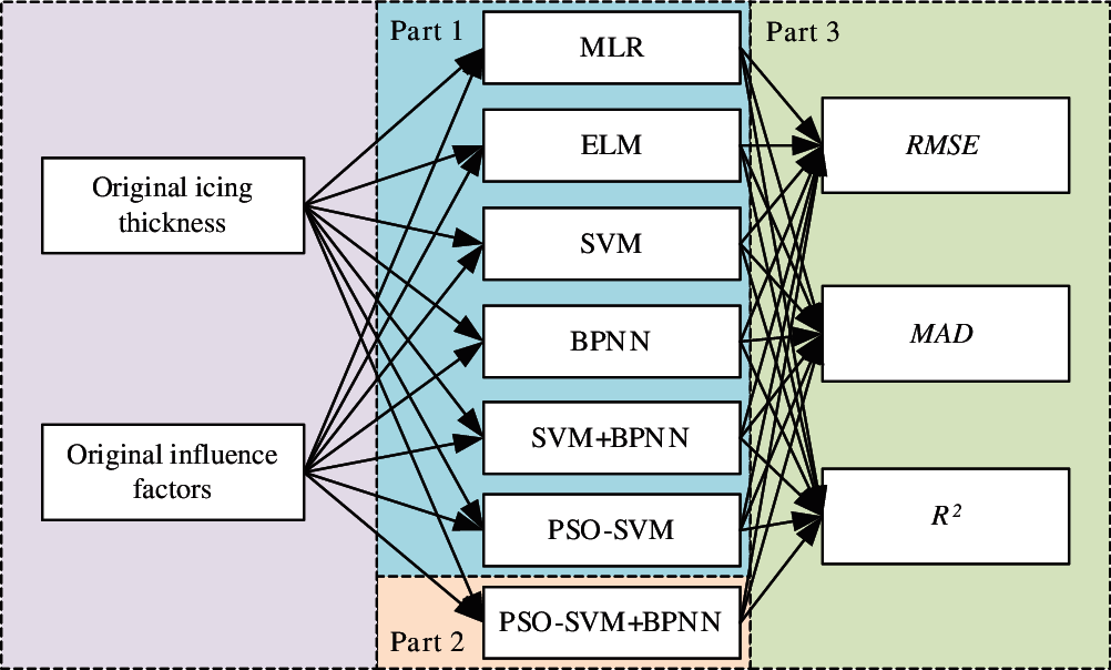
Figure 7: Framework of the diagnosis model comparisons

4.2 Icing Thickness Diagnosis

The icing thickness diagnosis results obtained using the seven models at 0.75R distance from the blade root of the wind turbine are shown in Fig. 8. Overall, the diagnosed results of MLR are quite different from the actual values. Fig. 8 shows a significant deviation in the diagnosis results obtained using the ELM, SVM, and BPNN models. The hybrid diagnosis model comprising of SVM+BPNN model reduces the sensitivity of a single diagnosis method. The comparison between the diagnosis results of PSO-SVM and SVM shows that the particle swarm algorithm significantly reduces the diagnosis error of the SVM model. Based on a comparative analysis of all the seven models, the hybrid diagnosis model comprising of PSO-SVM+BPNN yielded the best fitting performance and is the final model recommended from this paper.

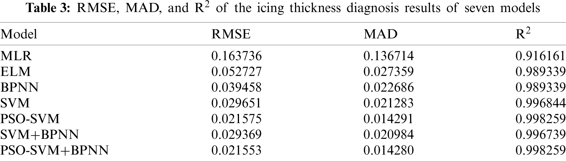
The study compared RMSE, MAD, and R2 of the ice thickness diagnosis results of all the seven models. As shown in Tab. 3, (a) the RMSE of models MLR, ELM, BPNN, and SVM is 0.163736, 0.052727, 0.039458, 0.029369, respectively; (b) MAD is 0.136714, 0.027359, 0.022686, and 0.01283, respectively; and, (c) R2 is 0.916161, 0.989339, 0.989339 and 0.996844, respectively. The RMSE and MAD of MLR are the highest and vice for the R2 value (i.e., the lowest) – which statistically indicates the poorest fitting for the regression functional model. When comparing a single diagnosis model, the rank order of model diagnosis accuracy from the highest (best) to lowest (poorest) is as follows: SVM, BPNN, ELM, and MLR, respectively. Compared to the SVM diagnosis results, the RMSE and MAD of PSO-SVM declined by about 0.008076 and 0.006992, respectively, ultimately indicating an improvement in accuracy. From these results, it is apparent that the particle swarm algorithm plays an important role in the optimization and diagnosis of the SVM model.

In comparison to the SVM and BPNN models, the RMSE of the SVM+BPNN hybrid diagnosis model decreased by about 0.000282 and 0.01089, respectively, whilst the MAD declined by about 0.000299 and 0.001702, respectively–which evidently indicates a further improvement in the model diagnosis accuracy. From the results in Tab. 3, the RMSE and MAD of the PSO-SVM+BPNN hybrid model are consistently the lowest with the highest R2, which proves the optimality of the model. The PSO-SVM+BPNN model combines the advantages of the two optimization methods, namely the SVM parametric optimization with PSO and dynamic weighted hybrid model, which has yielded satisfactory results in icing diagnosis.

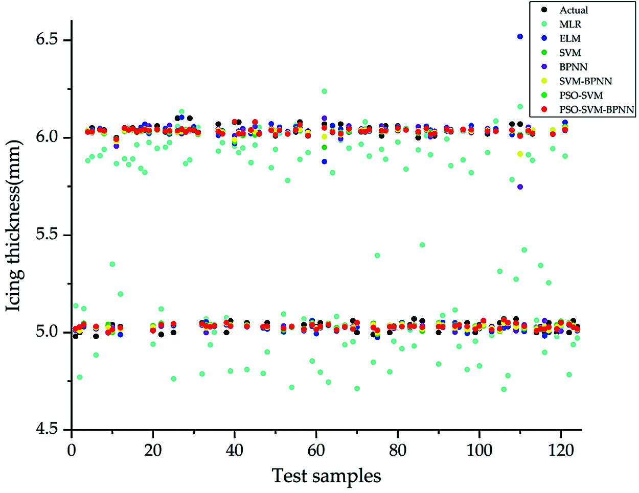
Figure 8: Icing thickness diagnosis of the seven models at 0.75R away from the blade root

5  Verification and Validation Simulations

This paper selected icing data at other locations of the wind turbine blades as a simulation case study to verify the applicability of the proposed model for diagnosing icing at different locations of wind turbine blades. This case study also allowed to further enhance and verify the accuracy of the diagnosis model. The measuring point of the icing thickness was selected at the leading edge of the blade. The distances from the root of the blade were 0.25R and 0.5R, respectively. The 324 sets of data were collected at each measuring point, of which the first 200 sets of data were training samples whilst the last 124 sets of data constituted the test samples. The environmental factors were similar to the previous case studies discussed in Section 4 of this paper. The collected data of the icing thickness at 0.25R and 0.5R away from the root are shown in Fig. 9 and Fig. 10, respectively.

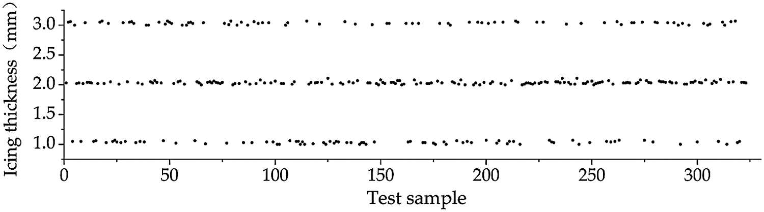
Figure 9: Data collection of the icing thickness at 0.25R away from the blade root

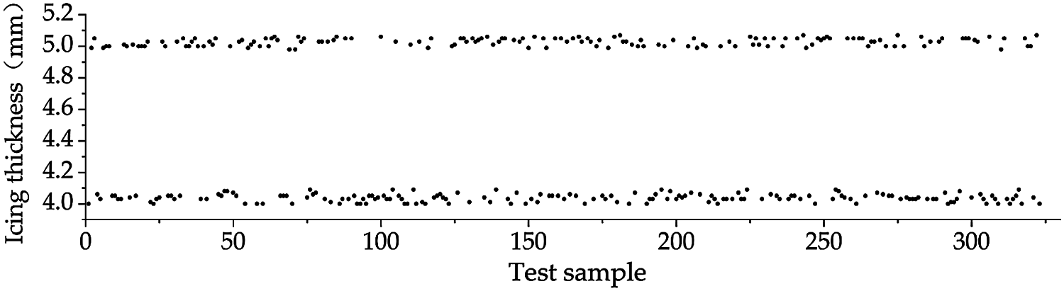
Figure 10: Data collection of the icing thickness at 0.5R away from the blade root

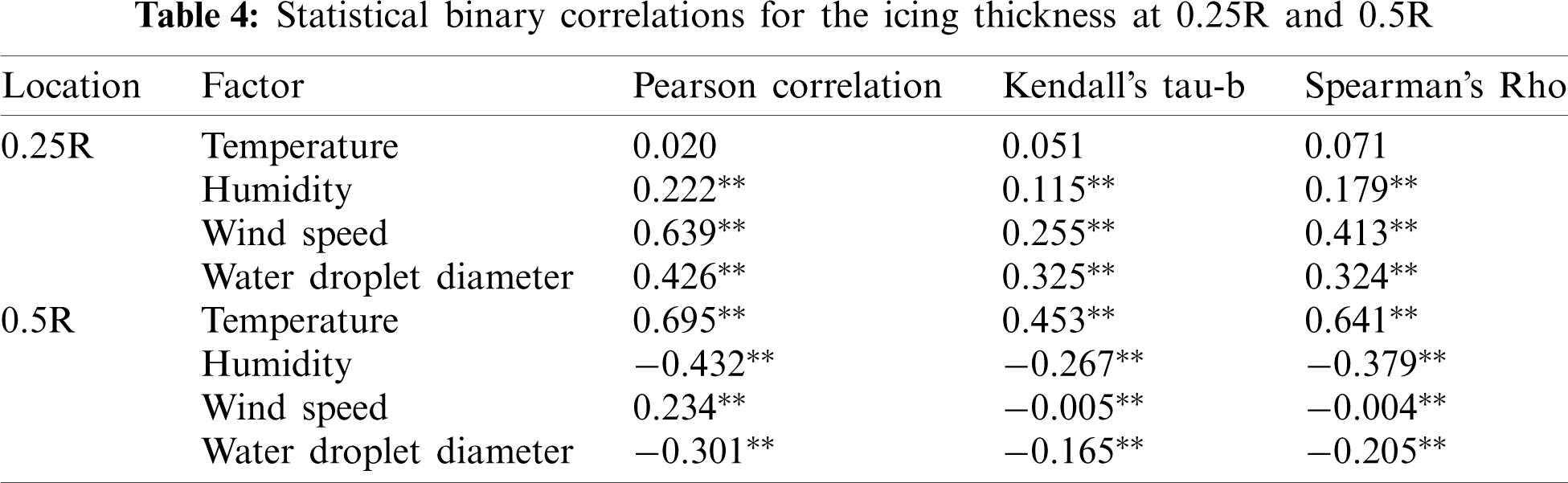
A statistical binary correlation analysis was performed on the selected icing factors of the wind turbine blade. As shown in Tab. 4, the statistical results show that each factor is closely related to the icing thickness.

The diagnosis results of the icing thickness on the front edge of the wind turbine blade at 0.25R and 0.5R of the seven models are as shown in Figs. 11–12, and Tab. 5, respectively. It can be seen from these results that the findings and conclusion obtained are consistent with the previous results discussed in Section 4 of this paper. In the single diagnosis model, MLR has the lowest diagnostic fit whilst ELM and BPNN have the largest errors in diagnosing local icing. In diagnosing the icing thickness of the wind turbine blade, PSO plays a significant role in the optimization of the SVM parameters and the kernel function. From these results, it is evident that the diagnosis effects of PSO-SVM are not only better than SVM and BPNN individually but also better than the performance of the SVM+BPNN combined forecasting model.

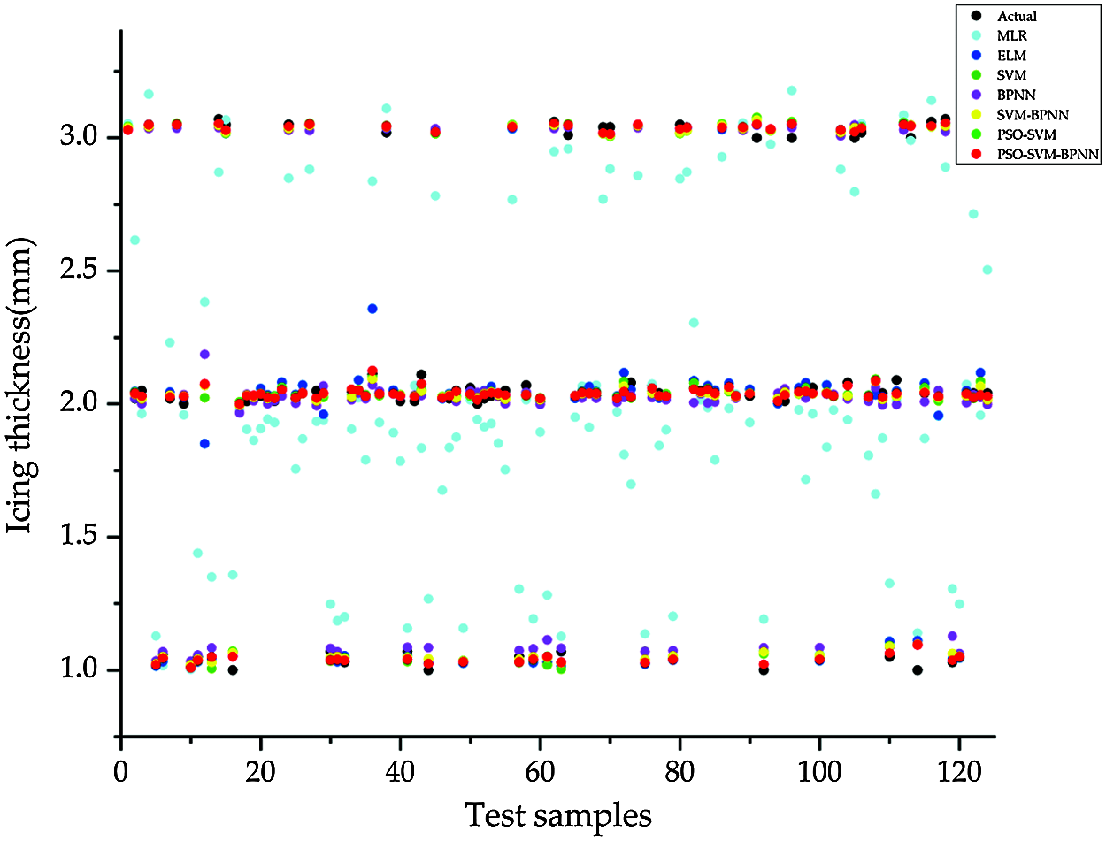
Figure 11: The icing thickness diagnosis of the models at 0.25R away from the blade root

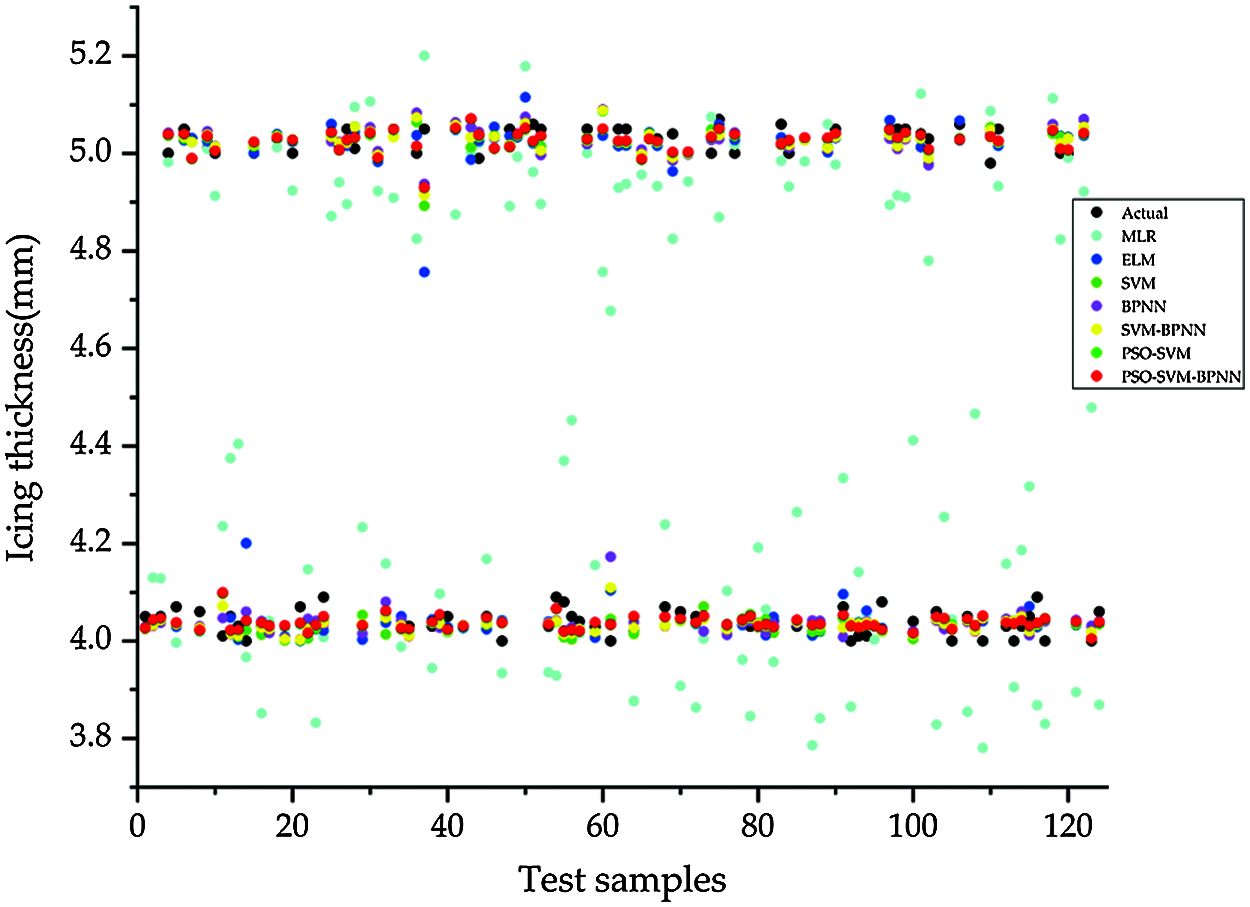
Figure 12: The icing thickness diagnosis of the models at 0.5R away from the blade root

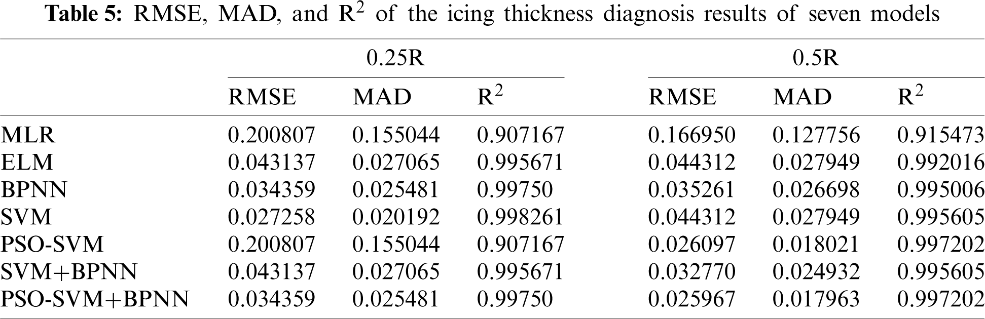
The diagnosis results of the SVM and BPNN models at 0.5R evaluated using the RMSE and MAD parameters show that the RMSE and MAD of BPNN are smaller than that of SVM. However, the results are opposite at 0.25R. Comparative analysis with single SVM and BPNN models proves that the hybrid diagnosis model comprising of SVM+BPNN has relatively lower RMSE and MAD, which ultimately improves the accuracy of the diagnosis results. (d) In the two diagnosis scenarios, the hybrid diagnosis model comprising of PSO-SVM+BPNN had the best regression fitting and the lowest deviation for the icing thickness analysis.

6  Conclusions and Recommendations

To achieve an accurate and stable diagnosis of the wind turbine blade icing, a dynamic weighted hybrid diagnosis model based on the PSO-SVM and BPNN formulation was proposed and successfully verified in this paper. The key findings drawn from the study are listed below:

(1)   Based on the outdoor natural environment and experimental data, the characteristic indicators of the environmental factors were extracted using binary correlation analysis of the environmental factors that affected the wind turbine blade icing. These factors included temperature, humidity, wind speed, and water drop diameter, which were used to analyze the wind turbine blades’ icing characteristic.

(2)   Through analysis of the training data that were obtained from the experiment, a PSO-SVM+BNPP combined model is proposed herein for diagnosing and analyzing the icing state of wind turbine blades. Based on the diagnostic analysis of the ice thickness for 0.75R, 0.25R, and 0.5R from the blade root of the wind turbine, the RMSE was found to be less than 0.026, MAD less than 0.018, and R2 less than 0.999. This proved and demonstrated that the diagnostic results of the combined model were more accurate and reliably superior.

(3)   When comparing the PSO-SVM+BNPP combined model with the MLR, ELM, BPNN, SVM, PSO-SVM, and SVM+BPNN models for blade icing thickness diagnosis at 0.75R, 0.25R, and 0.5R from the blade root of the wind turbine based on RMSE, MAD and R2 parameters, the hybrid prediction model, namely PSO-SVM+BPNN, yielded best regression fitting and the lowest deviation for the icing thickness prediction.

The icing on wind turbine blades has a detrimental effect on the power generation efficiency and operational safety of wind turbines. Based on environmental factors that can easily be obtained from wind farms, the models proposed in this paper indicated suitability to diagnose the thickness of icing on wind turbine blades. A comparison with the surface contact or embedded sensor diagnosis schemes showed that mitigating icing on wind turbines reduces the operational difficultness and production/maintenance costs, as well as minimizing/preventing the damage to the surface and internal structure of the wind turbine blades. The research work presented in this paper provides valuable decision support for wind farm operations and maintenance during winter.

Author Contributions: In this research activity, all the authors were involved in the experiment design and implementation, data analysis and preprocessing phase, results for analysis and discussion, and manuscript preparation. Xiyang Li conceived the experiment of ice coating on the wind turbine blade, designed research methodology, and participated in data analysis work. Bin Cheng guided the whole idea and framework of the paper and provided a lot of t revised opinions for the paper. Hui Zhang was mainly responsible for analyzing and discussing the experimental results, wrote and revised this paper. Xianghan Zhang conducted data collection and analysis. Zhi Yun presented the published work, specifically visualization.

Funding Statement: This work is supported by the Natural Science Foundation of China (Project No. 51665052).

Conflicts of Interest: We declare that we do not have any commercial or associative interest that represents a conflict of interest in connection with the work submitted. The founders had no role in the design of the study; in the collection, analyses, or interpretation of data; in the writing of the manuscript, or in the decision to publish the results.

References

 1.  Rastayesh, S., Long, L., Dalsgaard Sørensen, J., Thöns, S. (2019). Risk assessment and value of action analysis for icing conditions of wind turbines close to highways. Energies, 12(14), 2653. DOI 10.3390/en12142653. [Google Scholar] [CrossRef]

 2.  Frohboese, P., Anders, A. (2007). In effects of icing on wind turbine fatigue loads. Journal of Physics: Conference Series, 75(1), 12061–12073. DOI 10.1088/1742-6596/75/1/012061. [Google Scholar] [CrossRef]

 3.  Dolinski, L., Krawczuk, M. (2020). Analysis of modal parameters using a statistical approach for condition monitoring of the wind turbine blade. Applied Sciences, 10(17), 5878. DOI 10.3390/app10175878. [Google Scholar] [CrossRef]

 4.  Skrimpas, G. A., Kleani, K., Mijatovic, N., Sweeney, C. W., Jensen, B. B. et al. (2016). Detection of icing on wind turbine blades by means of vibration and power curve analysis. Wind Energy, 19(10), 1819–1832. DOI 10.1002/we.1952. [Google Scholar] [CrossRef]

 5.  Kabardin, I., Meledin, V., Dvoinishnikov, S., Naumov, I. (2016). Remote monitoring of ice loading on wind turbine blades based on total internal reflection. Journal of Engineering Thermophysics, 25(4), 504–508. DOI 10.1134/S181023281604007X. [Google Scholar] [CrossRef]

 6.  Neumayer, M., Bretterklieber, T., Flatscher, M. (2018). Signal processing for capacitive ice sensing: Electrode topology and algorithm design. IEEE Transactions on Instrumentation and Measurement, 68(5), 1458–1466. DOI 10.1109/TIM.19. [Google Scholar] [CrossRef]

 7.  Filippatos, A., Dannemann, M., Nguyen, M., Brenner, D., Gude, M. (2020). Influence of ice accumulation on the structural dynamic behaviour of composite rotors. Applied Sciences, 10(15), 5063. DOI 10.3390/app10155063. [Google Scholar] [CrossRef]

 8.  Zhang, Z., Zhou, W., Li, H. (2020). Icing estimation on wind turbine blade by the interface temperature using distributed fibre optic sensors. Structural Control and Health Monitoring, 27(6), 2534. DOI 10.1002/stc.2534. [Google Scholar] [CrossRef]

 9.  Muñoz, C. Q. G., Márquez, F. P. G., Tomás, J. M. S. (2016). Ice detection using thermal infrared radiometry on wind turbine blades. Measurement, 93, 157–163. DOI 10.1016/j.measurement.2016.06.064. [Google Scholar] [CrossRef]

10. Villalpando, F., Reggio, M., Ilinca, A. (2016). Prediction of ice accretion and anti-icing heating power on wind turbine blades using standard commercial software. Energy, 114, 1041–1052. DOI 10.1016/j.energy.2016.08.047. [Google Scholar] [CrossRef]

11. Makkonen, L., Laakso, T., Marjaniemi, M., Finstad, J. K. (2001). Modelling and prevention of ice accretion on wind turbines. Wind Engineering, 25(1), 3–21. DOI 10.1260/0309524011495791. [Google Scholar] [CrossRef]

12. Dierer, S., Oechslin, R., Cattin, R. (2011). Wind turbines in icing conditions: Performance and prediction. Advances in Science and Research, 25(1), 245–250. DOI 10.5194/asr-6-245-2011. [Google Scholar] [CrossRef]

13. Cao, Y., Yuan, K., Li, G. (2011). Effects of ice geometry on airfoil performance using neural networks prediction. Aircraft Engineering and Aerospace Technology, 83(5), 266–274. DOI 10.1108/00022661111159870. [Google Scholar] [CrossRef]

14. Kusiak, A., Verma, A. (2012). A data-mining approach to monitoring wind turbines. IEEE Transactions on Sustainable Energy, 3(1), 150–157. DOI 10.1109/TSTE.2011.2163177. [Google Scholar] [CrossRef]

15. Davis, N., Hahmann, A. N., Clausen, N. E., Žagar, M. (2014). Forecast of icing events at a wind farm in Sweden. Journal of Applied Meteorology and Climatology, 53(2), 262–281. DOI 10.1175/JAMC-D-13-09.1. [Google Scholar] [CrossRef]

16. Gantasala, S., Luneno, J. C., Aidanpää, J. O. (2017). Investigating how an artificial neural network model can be used to detect added mass on a non-rotating beam using its natural frequencies: A possible application for wind turbine blade ice detection. Energies, 10(2), 184. DOI 10.3390/en10020184. [Google Scholar] [CrossRef]

17. Zhang, L., Liu, K., Wang, Y., Omariba, Z. B. (2018). Ice detection model of wind turbine blades based on random forest classifier. Energies, 11(10), 2548. DOI 10.3390/en11102548. [Google Scholar] [CrossRef]

18. Zhou, G. F., Tan, W., Zhang, D. (2018). In ice detection for wind turbine blades based on PSO-SVM method. Journal of Physics: Conference Series, 2018, 22036. DOI 10.1088/1742-6596/1087/2/022036. [Google Scholar] [CrossRef]

19. Li, T., Tan, W., Liu, Z. (2019). A hybrid model based on logistic regression algorithm and extraction algorithm using reward extremum to real-time detect blade icing alarm. International Journal of Pattern Recognition and Artificial Intelligence, 33(14), 1955016. DOI 10.1142/S0218001419550164. [Google Scholar] [CrossRef]

20. Peng, C., He, J., Chi, H., Yuan, X., Deng, X. (2019). Icing prediction of fan blade based on a hybrid model. International Journal of Performability Engineering, 1(11), 2882–2890. DOI 10.23940/ijpe.19.11.p6.28822890. [Google Scholar] [CrossRef]

21. Kreutz, M., Ait-Alla, A., Varasteh, K., Oelker, S., Greulich, A. et al. (2019). Machine learning-based icing prediction on wind turbines. Procedia CIRP, 81, 423–428. DOI 10.1016/j.procir.2019.03.073. [Google Scholar] [CrossRef]

22. Yang, X., Ye, T., Wang, Q., Tao, Z. (2020). Diagnosis of blade icing using multiple intelligent algorithms. Energies, 13(11), 2975. DOI 10.3390/en13112975. [Google Scholar] [CrossRef]

23. Xu, X., Niu, D., Fu, M., Xia, H., Wu, H. (2015). A multi time scale wind power forecasting model of a chaotic echo state network based on a hybrid algorithm of particle swarm optimization and tabu search. Energies, 8(11), 12388–12408. DOI 10.3390/en81112317. [Google Scholar] [CrossRef]

24. Rayala, S. S., Kumar, N. A. (2020). Particle swarm optimization for robot target tracking application. Materials Today: Proceedings, 33(7), 3600–3603. DOI 10.1016/j.matpr.2020.05.660. [Google Scholar] [CrossRef]

25. Kaloop, M. R., Kumar, D., Zarzoura, F., Roy, B., Hu, J. W. (2020). A wavelet-particle swarm optimization-extreme learning machine hybrid modeling for significant wave height prediction. Ocean Engineering, 213, 107777. DOI 10.1016/j.oceaneng.2020.107777. [Google Scholar] [CrossRef]

26. Piotrowski, A. P., Napiorkowski, J. J., Piotrowska, A. E. (2020). Population size in particle swarm optimization. Swarm and Evolutionary Computation, 58, 100718. DOI 10.1016/j.swevo.2020.100718. [Google Scholar] [CrossRef]

27. Kumar, N., Dilawari, V., Bansal, A. (2020). Chemical equilibrium analysis of energetic materials using particle swarm optimization. Fluid Phase Equilibria, 522, 112738. DOI 10.1016/j.fluid.2020.112738. [Google Scholar] [CrossRef]

28. Li, D., Huang, F., Yan, L., Cao, Z., Chen, J. et al. (2019). Landslide susceptibility prediction using particle-swarm-optimized multilayer perceptron: Comparisons with multilayer-perceptron-only, BP neural network, and information value models. Applied Sciences, 9(18), 3664. DOI 10.3390/app9183664. [Google Scholar] [CrossRef]

29. Lorestani, A., Ardehali, M. (2018). Optimal integration of renewable energy sources for autonomous tri-generation combined cooling, heating and power system based on evolutionary particle swarm optimization algorithm. Energy, 145, 839–855. DOI 10.1016/j.energy.2017.12.155. [Google Scholar] [CrossRef]

30. Salahshoor, K., Kordestani, M., Khoshro, M. S. (2010). Fault detection and diagnosis of an industrial steam turbine using fusion of SVM (support vector machine) and ANFIS (adaptive neuro-fuzzy inference system) classifiers. Energy, 35(12), 5472–5482. DOI 10.1016/j.energy.2010.06.001. [Google Scholar] [CrossRef]

31. Eskandari, A., Milimonfared, J., Aghaei, M., Reinders, A. H. M. E. (2020). Autonomous monitoring of line-to-line faults in photovoltaic systems by feature selection and parameter optimization of support vector machine using genetic algorithms. Applied Sciences, 10(16), 5527. DOI 10.3390/app10165527. [Google Scholar] [CrossRef]

32. Krama, A., Zellouma, L., Rabhi, B., Refaat, S. S., Bouzidi, M. (2018). Real-time implementation of high performance control scheme for grid-tied PV system for power quality enhancement based on MPPC-sVM optimized by PSO algorithm. Energies, 11(12), 3516. DOI 10.3390/en11123516. [Google Scholar] [CrossRef]

33. Baser, F., Demirhan, H. (2017). A fuzzy regression with support vector machine approach to the estimation of horizontal global solar radiation. Energy, 123, 229–240. DOI 10.1016/j.energy.2017.02.008. [Google Scholar] [CrossRef]

34. Çelikyılmaz, A., Türkşen, I. B. (2007). Fuzzy functions with support vector machines. Information Sciences, 177(23), 5163–5177. DOI 10.1016/j.ins.2007.06.022. [Google Scholar] [CrossRef]

35. Gu, L., Han, Y., Wang, C., Shu, G., Feng, J. et al. (2018). Inventory prediction based on backpropagation neural network. NeuroQuantology, 16(6), 664–673. DOI 10.14704/nq. [Google Scholar] [CrossRef]

36. Jiao, A., Zhang, G., Liu, B., Liu, W. (2020). Prediction of manufacturing quality of holes based on a BP neural network. Applied Sciences, 10(6), 2108. DOI 10.3390/app10062108. [Google Scholar] [CrossRef]

37. Zeng, Y. R., Zeng, Y., Choi, B., Wang, L. (2017). Multifactor-influenced energy consumption forecasting using enhanced back-propagation neural network. Energy, 127, 381–396. DOI 10.1016/j.energy.2017.03.094. [Google Scholar] [CrossRef]

38. Liu, Z., Liu, X., Wang, K., Liang, Z., Correia, J. A. et al. (2019). GA-Bp neural network-based strain prediction in full-scale static testing of wind turbine blades. Energies, 12(6), 1026. DOI 10.3390/en12061026. [Google Scholar] [CrossRef]

39. Dong, S., Zhang, Y., He, Z., Deng, N., Yu, X. et al. (2018). Investigation of support vector machine and back propagation artificial neural network for performance prediction of the organic rankine cycle system. Energy, 144, 851–864. DOI 10.1016/j.energy.2017.12.094. [Google Scholar] [CrossRef]

40. Kollar, L. E., Mishra, R. (2019). Inverse design of wind turbine blade sections for operation under icing conditions. Energy Convers Manage, 180, 844–858. DOI 10.1016/j.enconman.2018.11.015. [Google Scholar] [CrossRef]

This work is licensed under a Creative Commons Attribution 4.0 International License, which permits unrestricted use, distribution, and reproduction in any medium, provided the original work is properly cited.