Energy Engineering

DOI: 10.32604/EE.2021.015602

ARTICLE

Load Forecasting of the Power System: An Investigation Based on the Method of Random Forest Regression

Fuyun Zhu and Guoqing Wu*

College of Mechanical and Electrical Engineering, Soochow University, Suzhou, 215137, China
*Corresponding Author: Guoqing Wu. Email: wgq@ntu.edu.cn
Received: 30 December 2020; Accepted: 08 March 2021

1  Introduction

Energy is essential for the sustainable development of the society. Over the past decades, global energy demand has experienced a vigorous growth [1]. It is noticed that most of the energy currently consumed is from fossil fuels, which has caused many environmental pollutions [2]. The electricity, as an efficient and clean energy, plays a more and more significant role in the industrial production and daily life in the form of special commodity [3,4].

Accurate load prediction can alleviate the contradiction between supply and demand of power [5]. Due to the particularity of power storage, the generated power needs to be consumed in time, otherwise this could damage the power system to affect people’s daily life, for instance, the widespread power outage of the interconnected power grid of eastern Canada and northeastern United States on August 14, 2003 and the accidental collapse of the power grid on July 30, 2012 in nine northern states in India [6,7]. In order to reduce the power loss and improve the security and stability of grids, it is very important to forecast the power load and make reasonable dispatching plans in advance [8].

Since the power load often has a certain periodicity, it is feasible to be forecasted by some methods. Traditionally, the time-series models were widely used in power load forecasting. Ziel presented a simple quintile regression-based forecasting method that was applied in the probabilistic load forecasting framework of the Global Energy Forecasting Competition [9]. Lee et al. used a lifting scheme and autoregressive integrated moving average (ARIMA) models to achieve short-term load forecasting [10]. However, it is momentous to realize that the traditional time-series model only considers the relationship between the time and power load, which has obvious limitations in the prediction accuracy and stability because of the negligence caused by many other factors such as date, temperature and wind speed etc. With consideration of the above problems, the load forecasting method based on machine learning was proposed, for which some studies have been done by many researchers. The support vector machine regression model (SVR), the random forest regression (RFR) model and the neural network method (NN) are three mainstream machine learning methods for power load forecasting. Chen et al. used the SVR model to forecast the short-term power load demand of office building. The actual test showed that the prediction results had high accuracy and stability [11]. It should be noted that the prediction accuracy of SVR model was greatly affected by the algorithm itself and the selection of input features [12,13]. The RFR model could effectively avoid the above problems. Especially, all the features could be used to establish the prediction model [14]. Lv et al. predicted the power load of cities in North China based on the improved RFR model and the prediction results were satisfactory [15]. Azim et al. considered a variety of factors and designed a compound artificial neural network method for forecasting power load. Experimental results showed that the method designed by Azim et al. had a good reliability. But the model was still slightly complicated in the structure, which limited its further application [16,17].

From the above research results, it also appears that the selection of methods and the process of factors have become increasingly important. Generally speaking, the accuracy of prediction depends on the stationary input conditions. That is to say, machine learning methods have great potential to forecast the power load in the months with fewer special holidays. One example will suffice to illustrate the point. In China, it is suitable for forecasting power load during the period from May to September with fewer, but long enough special holidays are conducive to test the prediction accuracy of the model. Meanwhile, as we know, the energy consumption in building sector has accounted for the significant part of the energy in the world, of which the air conditioning equipment plays an important role in building energy consumption [18]. The time period for prediction in this study is in summer with the peak of electricity consumption. Thus, it may be helpful to improve the accuracy of power load forecasting by introducing some indexes in HVAC field and modifying the input system of machine learning method.

Overall, the purpose of this paper is to establish a mathematical model for forecasting the power load based on the RFR model. Then, several other main machine learning models will be compared with the established RFR model and the performance will be evaluated based on statistical indicators. Finally, the impacts of the air conditioning system on the power load will be discussed.

2  Data Preparation and Cleaning

The load data used in this study were obtained from the Electrician Mathematical Contest in Modeling of Chinese society for electrical engineering, which was provided in literature [15]. The power loads were measured over the course of almost 3 years, from 2012-01 to 2015-01. Figs. 1 and 2 show the sampling results of daily loads from May 21, 2012 to May 27 (from Monday to Sunday), 2012 and the monthly loads in January and February 2013 respectively. It can be found from Monday to Saturday that the curves of the daily load increase fast from 7 a.m. to 10 a.m., 12 a.m. to 16 p.m. and 18 p.m. to 21 p.m.. The first two period are working time. During the third time period, people are mainly having a rest at home. However, people do not go to work on Sundays, which makes the electricity load drop significantly. But the curve still has three obvious peaks, and the time periods of the peaks are similar to the working day. Due to the concentration of using electricity, there are three peaks in these time periods.

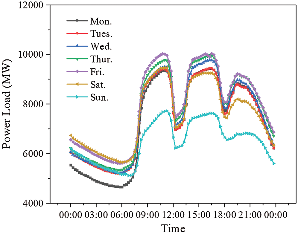
Figure 1: The curves of daily change for power loads

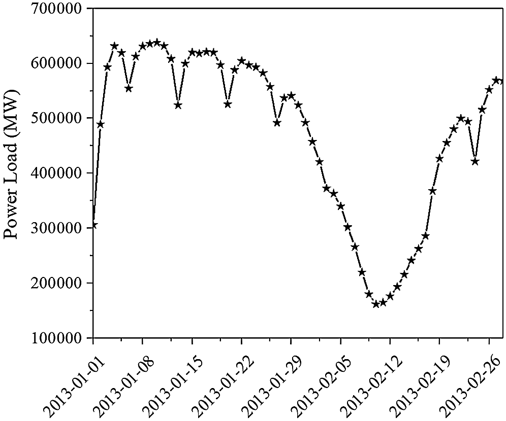
Figure 2: The curve of monthly change for power loads

Despite of some slight fluctuations during these periods, the curves were generally maintained at a high level. In the rest of the time periods, the load curves remained at a relatively low level.

It can also be noted that the curve of monthly loads shows a regular distribution. The power loads during the working days are always higher than those on holidays, especially in February when the lunar New Year begins. It should be noted that after the Spring Festivals, the curve of power loads increase to the normal level quickly.

As can be known from the above analysis that the load of the power system was not only influenced by the factors such as the weather, temperature, holiday and vacations, etc., the date characteristic also have marked impacts on the power load, which shall be taken into account in the study.

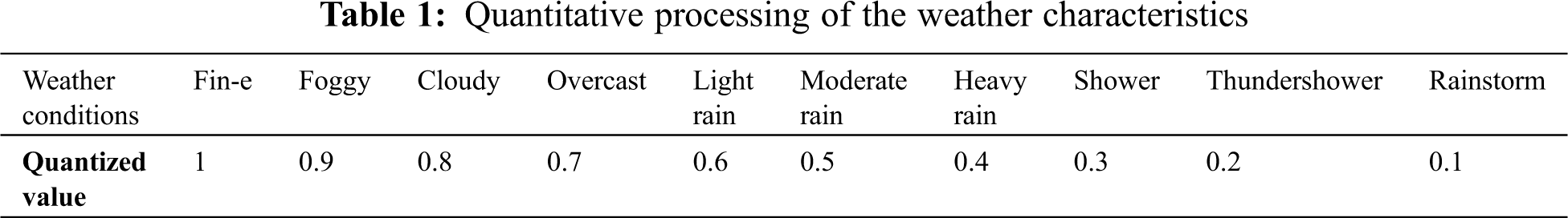
According to the study of Sui [19], the weather factors always contained many random errors. In order to obtain stable data sets, it is necessary to quantify these factors. Besides, the historical data of the load in power system in this study are mainly concentrated in summer. Thus, the weather factors can be quantified as shown in Tab. 1.

Due to different statistical standards, there is a considerable difference in the factors like temperature, humidity, wind speed, etc., from which the differences in characteristic values are eliminated based on the method data standardization to obtain the formula for the method as follows:

S′=S−mstd (1)

where S′ is the normalized sequence, S is the characteristic sequence, m and std are the average value and standard deviation of the sequence respectively.

Generally, date characteristic is always discrete. Considering the fact that there is also a big gap in the electricity load demand between holidays and working days, it is necessary to take the date as an important variable in forecasting models. Since several special holidays like Dragon Boat Festival, Mid-Autumn Festival etc. were not considered in this study, the value on the working days shall be set as 0 and it on the weekend shall be set as 1.

The wide application of the air conditions in summer is also an important reason for the increase of power loads. Actually, whether people use air conditionings or not often depends on environmental variables. The environmental factors of the comprehensive environmental index (CE) and Comprehensive comfort index (CC) can be used to reflect the use of air conditionings and other refrigeration equipment indirectly, for which the formulas can be written as [20,21]:

CE=37−37−T0.68−0.14H+1/(1.76+1.4V0.75)−0.29T(1−H) (2)

CC=1.8T+0.55(1−H)−3.2V+27 (3)

where T is the average daily air temperature (°C), H is the average daily relative humidity (%), and V is the average daily wind speed (m/s).

3  Characteristic Analysis and Algorithm Design

With the data processed, a new prediction model considering various factors for the power loads based on the random forest regression (RFR) can be set up, of which the RFR is an ensemble learning algorithm that allows considering the regression problems and the classification problems in single or multiple frameworks. It mainly consists of a pair of random regression trees (RT) that can be operated for making multiple regression trees and making predictions. By collecting quite a few trees and finding the error rates to select the most suitable tree, the Bagging Algorithm shall be adopted to draw samples from the test set and the formula for the error rate can be written as:

min(MSE)≈min(MSEbag)=min{1s∑i=1s(1m∑j=1myj−yi)2}=min{1s∑i=1s(1m∑j=1mBRTj(xi)−yi)2} (4)

where s is the number of samples, MSE is the mean square error, MSEbag is the MSE of bag; yj, BRTj(xi) is the predictive value of the j-th RT; yi and xi are the i-th value of the characteristics and the i-th value of the real power load. For the final predictive power loads y(R), it can be written as:

y(R)=1m∑q=1m∑t∈RT:v(st)=xiRFC(q)yq(st,t)=1m∑q=1myq(R) (5)

where C(q) is the sum of correlation coefficients of the q-th RT. Actually, the parameter setting of model can also influence the accuracy of predictive values. For the RFR, the number of the RT (m), the number of the selected load characteristics (f) and the number of leaves for the RT (N) are the main three factors that have marked effects on the convergence of the model. There are two important parameters (m and N) in the RFR needed to be set since the selected load characteristics (f) has been determined. In fact, the number of leaves for the RT (N) needs to be adjusted when the RFR is used to deal with large data sets. That is to say, for the following study, as long as the values of m is adjusted suitably, the model with the best prediction performance can be obtained when N is left on the default parameters. Here the grid search algorithm (GSA) was used to search for the best parameter of m.

Generally, the higher the prediction accuracy of the model, the larger fitting degree between the simulated data and the measured data. The coefficient of determination (R2) can be used to describe this feature, that is:

R2=1−RSSTSS (6)

Considering the fact that the value of m needs to be adjusted to obtain a model with the best perdition performance, R2 can also be viewed as the fitness function for the RFR. By giving parameter ranges of m, then conducting the grid search algorithm, the result of R2 for each m can be obtained. The value of m corresponding to the maximum R2 is the best parameter. The distribution of R2 with different m and the flow chart for conducting the RFR can be seen in Figs. 3 and 4. As shown in the figures, when the value of m is 10, the R2 can reach 0.514, indicating that value of m is the best parameter for the model.

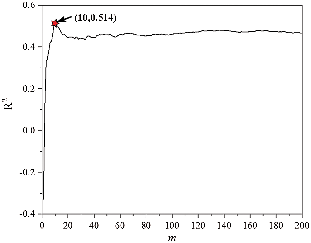
Figure 3: The distribution of R2 with different m

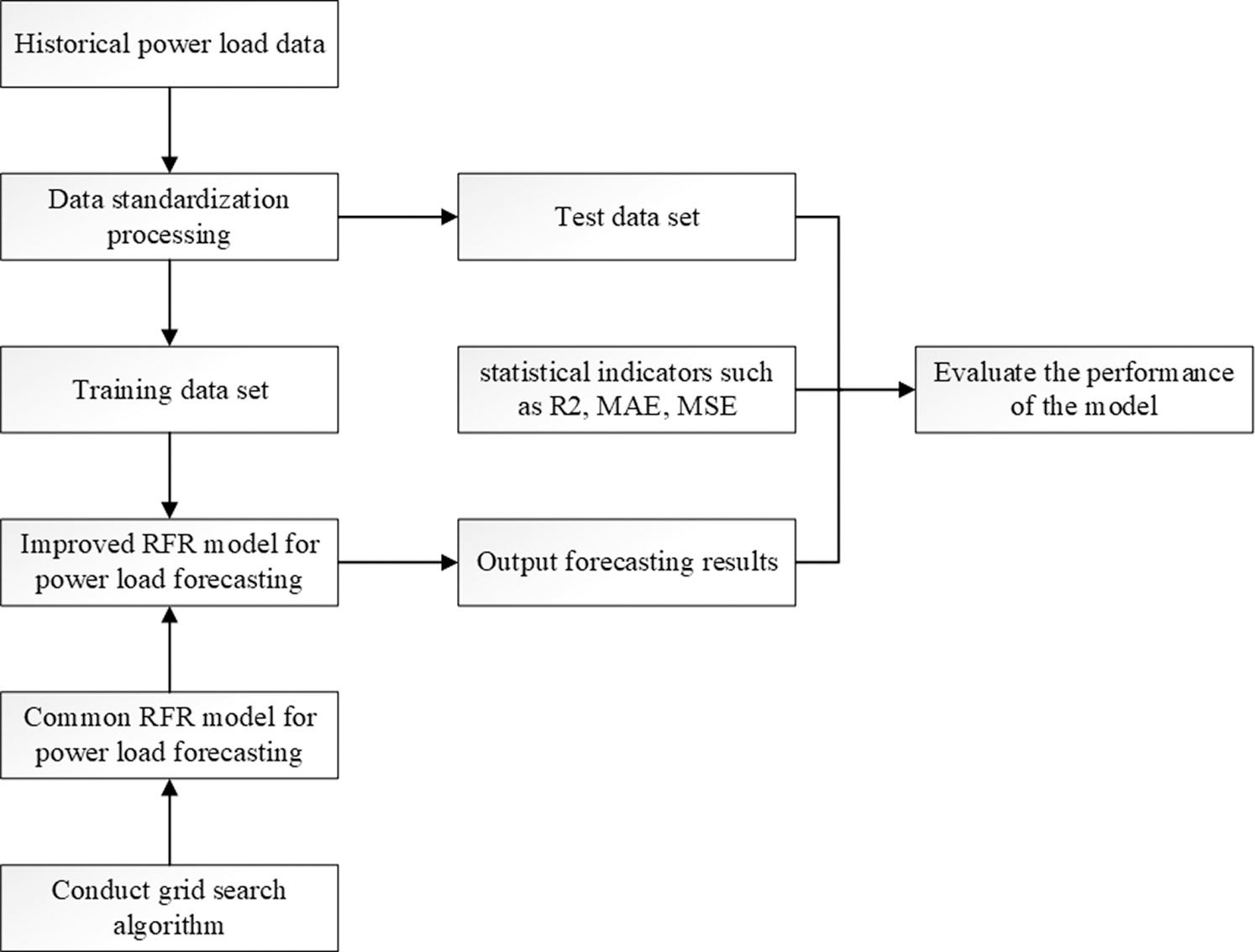
Figure 4: The flow chart for conducting the RFR model

Apart from the RFR, there are many other machine learning algorithms applied in the field of power loads forecasting widely, such as the artificial neural network (ANN), support vector regression (SVR), K-nearest neighbors (KNN), linear Regression (LR) and gradient boost regression tree (GBRT). For the prediction problems arising from using the method of machine learning, the following statistical indicators are most commonly used:

MAE=1m∑i=1m|(yi−y^i)| (7)

MSE=1m∑i=1m(yi−y^i)2 (8)

where MAE is the mean absolute error and MSE is the mean squared error. These indicators can be used to describe the degree of deviation between the simulated values and the measured values and the smaller the values of the indicators are, the smaller of the degree of deviation is. In the following study, these indicators will be used to evaluate the prediction performance of proposed method by conducting the comparison with these classical algorithms.

4  Case Study

4.1 Comparison of Results for Different Machine Learning Algorithms

In order to evaluate the performance of each model accurately, the data set were divided into training set and test set according to the principle of 8:2. For the RFR, the values of m and f are 10 and 7, respectively. As for the algorithms proposed above, the final results obtained from calculation are shown in Fig. 5.

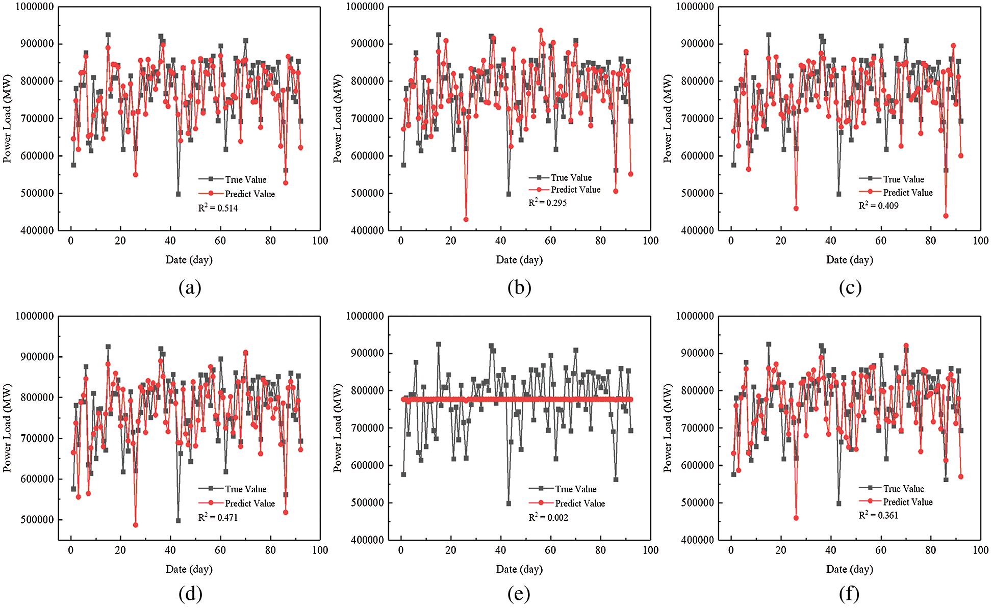
Figure 5: Comparison of results in test data set for different models (a) RFR (b) KNN (c) GBRT (d) LR (e) SVR (f) ANN

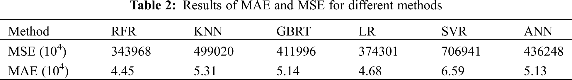
Obviously, it can be seen that the R2 with the model of the RFR is the largest, reaching 0.514. The results of LR are also higher than those of other models. It is worth noting that the result of SVR is the worst. The R2 is only 0.002 and the predictive curve almost remains a straight line, which means that the model of SVR is not suitable for the short-term load forecasting in this study. Also, the results of MAE and MSE are calculated. As can be seen in Tab. 2, the values of MSE and MAE for RFR are 3.44 × 109 and 4.45 × 104, respectively, which are still the smallest in the list, indicating that there are fewer data fluctuations in the simulated results for the RFR compared with those for other methods. Overall, the above calculated results show that the model of the RFR has the best predictive performance among these models.

4.2 Impacts for the Characteristics of Date and Environmental Factors

The accuracy of the RFR was verified by testing multiple machine learning models. Actually, the selections of characteristic also have marked impacts on the forecasting results. It is widely known that there is a wide variety of holidays in China. To alleviate the influence of these holidays, this study was concentrated on the forecast of the power system in summer. By researching on the load data of the power system concentrated from May to September, it can be found that some characteristics have a significant impact on the accuracy of the prediction results. As shown in Fig. 6, if date can be regarded as a characteristic, the fitting degree of the curve for the RFR can reach 0.514. Conversely, if not, the fitting degree of the curve is only 0.326.

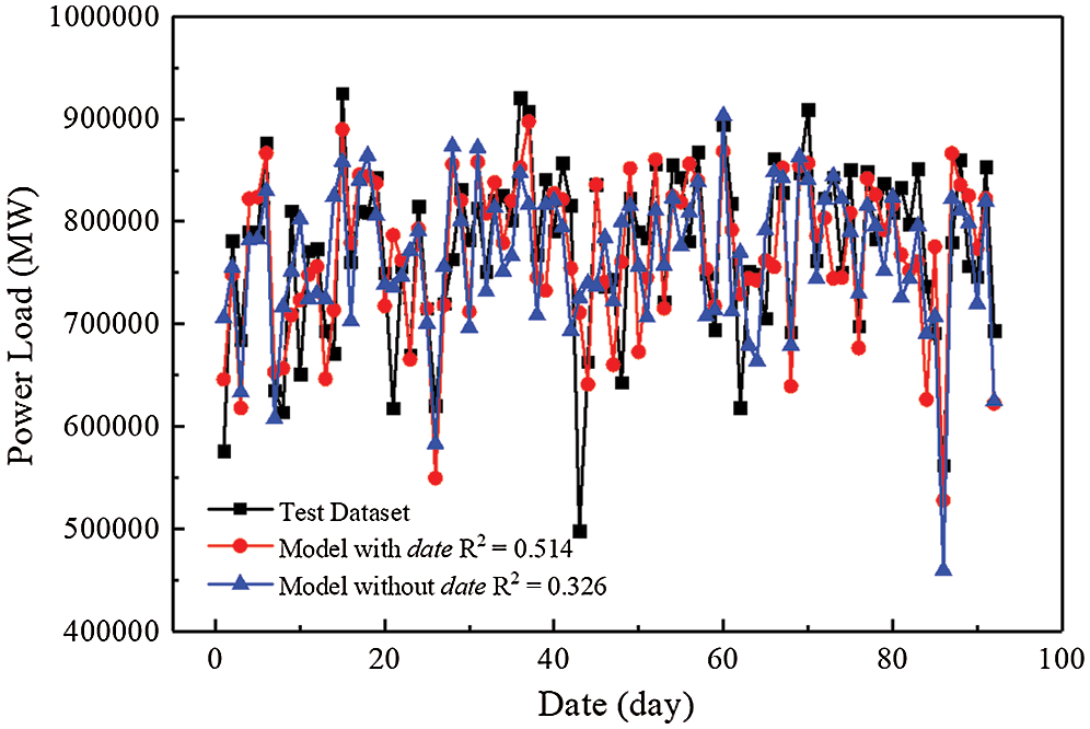
Figure 6: Comparison of results in test data set with different date characteristic

It can be further found that the curve containing the characteristic of date is in better agreement with the peaks and valleys of the measured data compared with the curve without date, especially when there is a big difference between the adjacent measured data, which may be caused by working days and weekends. From the Figs. 1 and 2, it can be observed that the electricity load varies greatly between weekdays and weekends. Although the period from May to September is the summer vacation for the students in China, this is still a normal working period for most people, which can explain why the RFR model considering the characteristic of date has a better prediction performance.

Some temperature-related data can be obtained from the measured data. Usually, the hotter it is, the more frequently air conditioning is used. It should be noted that the temperature difference varies greatly between day and night, together with the changing throughout the day. Besides, since this paper mainly focused on the impacts of the use of air conditioning equipment on electricity load, it is common knowledge that the use of air conditioner depends not only on temperature, but also on humidity, wind speed and other factors, which are called as thermal comfort index in the field of HVAC, and can be better used to assess whether people are more willing to use air conditioning, of which the environmental factors of the comprehensive environmental index (CE) and Comprehensive comfort index (CC) are viewed as two important indexes to evaluate the use of the air conditions. The RFR model was used to calculate the results with or without CE and CC, respectively, as shown in Fig. 7.

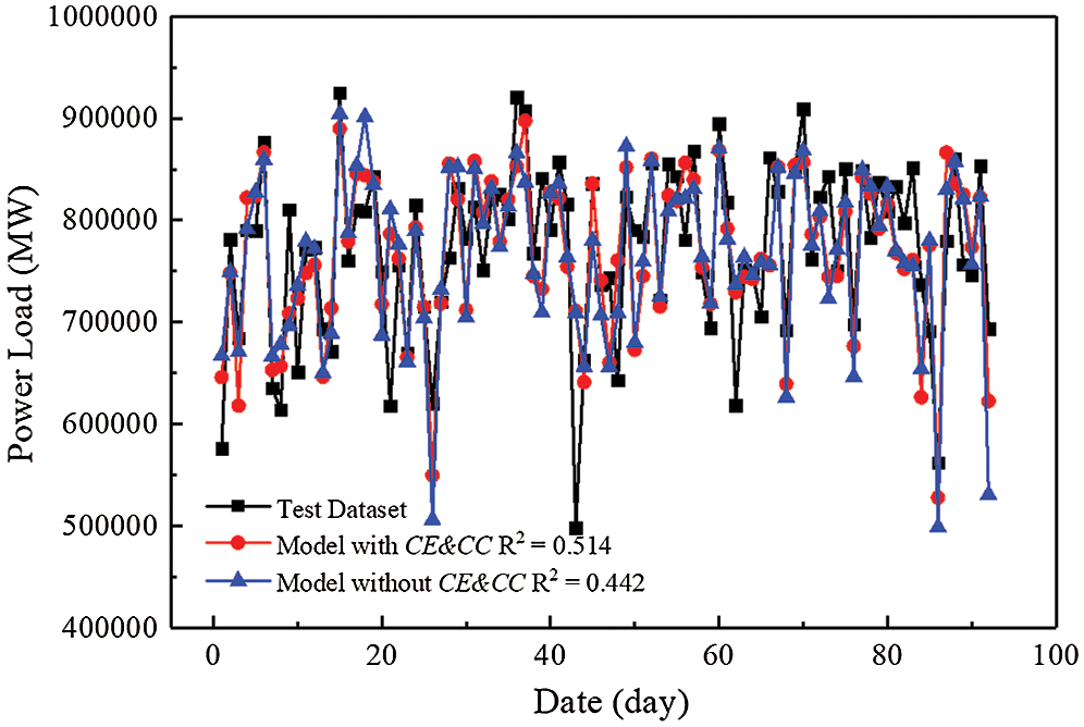
Figure 7: Comparison of results in test data set with different HVAC characteristic

From the above Figure, it is obvious that the two curves with or without CE and CC are very similar. The fitting degrees are both larger than 0.44, which agree with the measured data well. However, there are still some subtle differences between them. As shown in Fig. 7, at the valleys, the results for the RFR without CE and CC have some cases of over fitting. Compared with the results for the RFR with CE and CC, there is a great improvement for the fitness of the curve at the peaks. After querying the measured data, it can be found that when the average temperature and relative humidity are both high, the results predicted by the model differ greatly, especially on the working days. Combining with the above discussions about date, the reason for the difference of fitting degree between the curves with or without CE and CC may be answered. Due to the period for this study being a normal working period for most people, at the high temperature and relative humidity people are more likely to use air conditioners. The results for the RFR with CE and CC agree with the measured data better compared with those of the curve without CE and CC, indicating that the prediction accuracy of the electricity load for RFR can be improved effectively when two important factors of CE and CC taken into account. Undoubtedly, the wide use of air condition equipment in office buildings is an important factor in the increase of the electricity load.

5  Conclusion

Compared with several other common machine learning methods, the forecasting results for the established model has the highest R2, the lowest MAE and MSE on the test set, indicating that when the number of the RT (m) was 10, the model based on the RFR model had the best prediction performance.

After introducing two important indexes in HVAC, the accuracy of prediction has been improved obviously, which means that the wide use of air condition in office buildings is an important factor in the increase of the electricity load.

This paper focused on the modeling for power load forecasting based on the machine learning method. However, the forecasting result may be influenced by some other factors, requiring that further investigation on the effects from other influence factors shall be carried out in the future.

Funding Statement: This work was supported by National Natural Science Foundation of China (Grant 61273151).

Conflicts of Interest: The authors declare that they have no conflicts of interest to report regarding the present study.

This work is licensed under a Creative Commons Attribution 4.0 International License, which permits unrestricted use, distribution, and reproduction in any medium, provided the original work is properly cited.