Energy Engineering

DOI: 10.32604/EE.2021.015930

ARTICLE

A Novel Starting Impulse Suppression Method for Active Power Filter Based on Slowly Rising Curve

Jianfeng Yang* and Yu Ding

School of Automation and Electrical Engineering, Lanzhou Jiaotong University, Lanzhou, 730070, China
*Corresponding Author: Jianfeng Yang. Email: jfyang@mail.lzjtu.cn
Received: 24 January 2021; Accepted: 08 April 2021

1  Introduction

With the widespread application of high-power electronic devices in recent years, the number of nonlinear electronic devices in the power grid is increasing, leading to an increase in current harmonic pollution in the power grid. Harmonics affect power quality and threaten power system security and stability. Therefore, harmonic control has become a problem to solve in the rapid development of power electronic devices with nonharmonic being a sign of the green and healthy development of power systems [1,2]. The effect and performance of traditional passive power filters cannot meet the current demand, so a parallel active power filter is proposed. SAPF can realize real-time dynamic compensation of harmonics in the power grid, with a good governing effect, fast response speed, and flexible application, and has been widely used in power quality control [3–5].

In the process of grid-connected start-up, SAPF has the problems of DC side voltage overshoot and current surge. Voltage overshoot causes the voltage value on the switch device to exceed the maximum voltage that the switch device can withstand, resulting in damage to the switch device. Current surge has an impact on the stability and safety of the power grid. Therefore, it is necessary to design a reasonable starting strategy for the SAPF system and the security and stability of the power grid [6–10].

SAPF usually adopts a double closed-loop control mode, with voltage as the outer loop and current as the inner loop. This control mode is simple in structure and easy to realize in the digital system. However, due to the inherent characteristics of Proportion-Integral (PI) Control, there is a deviation between the actual value and the expected value of DC capacitor voltage at the moment of SAPF grid connection. For the controller, the expected value of voltage is equivalent to a step response: the actual value of voltage exceeds the expected value of voltage and results in a certain impulse voltage. The output of the controller in the outer voltage loop is in the form of current value, which further intensifies the current under the control of the inner current loop impact and affects the stability and safety of the system [11–13].

At present, the research on SAPF mainly focuses on the control strategy after stable operation of SAPF. For example, Hekss et al. used cascaded adaptive nonlinear controller based on state space model to solve the problem of photovoltaic system composed of SAPF [14]. Fang et al. proposed an adaptive canvas fuzzy neural network controller based on Fuzzy synovial control to improve the compensation performance of APF [15]. By analyzing the causes of DC bus fluctuation in SAPF under power balance scheme, Meng et al. proposed a feedforward channel method based on cascaded delay signal to reduce DC bus fluctuation and make SAPF better adapt to load change [16]. Al-Gahtani et al. proposed a frequency adaptive control method to deal with the influence of system frequency change on SAPF and ensure its stable operation [17]. Liu et al. proposed an adaptive fractional order synovial control scheme based on RBF neural network to improve the stability and robustness of the system [18]. The above research is mainly to improve the reliability and compensation performance of SAPF after starting, but the research on the starting stage of SAPF is less. Aiming at the current and voltage pulses generated in the start-up phase of SAPF, the causes of the pulses are analyzed, and a method of SAPF start-up pulse based on slow rising curve is designed, which can effectively suppress the current and voltage pulses generated in the start-up phase of SAPF.

The first chapter introduces the background and significance of the research. Chapter two establishes the mathematical model of the DC side SAPF. Chapter three analyzes the causes of the starting shock theoretically. In chapter four, an SAPF starting strategy based on the slow rising curve is proposed. In chapter five, the starting strategy proposed in chapter four is simulated and verified in MATLAB/Simulink. Chapter six summarizes the paper in its entirety.

2  Analysis of Impact Mechanism of SAPF

This paper uses three-phase three-wire SAPF as the research object. The system is mainly composed of a power grid, nonlinear load, and SAPF. The structure diagram is shown in Fig. 1 below. In the figure, ea, eb, and ec are grid voltage; ua, ub and uc are output voltage of three-phase voltage source inverter; iLa, iLb and iLc are nonlinear load current; ia, ib, and ic are three-phase grid current; ica, icb, and icc are harmonic compensation current of SAPF; R represents equivalent resistance of line, inductance, capacitance and loss of inverter itself; L is filter inductance; C is DC side capacitance; udc is DC side voltage [19].

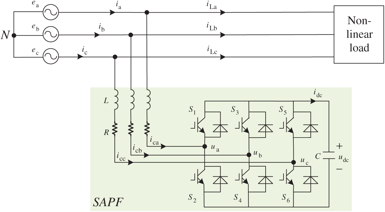
Figure 1: Three-phase three-wire SAPF schematic diagram SAPF

According to the SAPF topology in the figure above, it is shown that:

{Ldicadt+Rica=ea−(Sa−13∑j=a,b,cSj)udcLdicbdt+Ricb=eb−(Sb−13∑j=a,b,cSj)udcLdiccdt+Ricc=ec−(Sc−13∑j=a,b,cSj)udcCdudcdt=Saica+Sbicb+Scicc (1)

where Sj is the switching function of the phase bridge arm, j = a, b, c.

Sj={1The upper arm is on and the lower arm is off0The lower arm is on and the upper arm is off (2)

The coordinate transformation of Eq. (1) is carried out, and the three-phase coordinate system is transformed into the two-phase static coordinate system, The SAPF mathematical model under DQ coordinate axis is obtained, as shown in Eq. (3):

{LdiDdt+RicD=eD−SDudcLdiQdt+RicQ=eQ−SQudcCdudcdt=32(SDiD+SQiQ)  (3)

where SD and SQ are switching functions in the two-phase static coordinate system (D, Q).

Eq. (3) is further transformed into an SAPF mathematical model in the two-phase rotating coordinate system (d, q), as shown in Eq. (4):

{Ldicddt+Ricd−ωLicq=ed−SdudcLdicqdt+Ricq+ωLicd=eq−SqudcCdudcdt=32(Sdicd+Sqicq) (4)

where Sd and Sq are switching functions in the two-phase stationary coordinate system (d, q). icd and icq are dq axis components of the input grid current of SAPF.

In Eq. (4), the

If both sides multiply udc at the same time, the following Eq. (5) can be obtained:

Cudcdudcdt=32(udicd+uqicq) (5)

The above equation is discretized into:

udc(k)[Cudc(k)−udc(k−1)Ts]=32[ud(k)icd(k)+uq(k)icq(k)] (6)

where Ts is the sampling time [20].

In the transition phase, SAPF does not compensate the harmonics of the power grid, so icq = 0 can further transform Eqs. (6)–(7):

icd(k)=23udc(k)ud[Cudc(k)−udc(k−1)Ts] (7)

where ud is the d-axis component transformed from ua, ub, and uc, which can be obtained by further transforming Eq. (7):

icd(k)=23ud[Cudc2(k)−udc(k)udc(k−1)Ts] (8)

At this time, for k time, the value of k−1 time has been measured, which can be regarded as a constant.

Suppose:

M=2C3udTsN=udc(k−1) (9)

By introducing Eq. (9) into Eq. (8), one may get:

icd(k)=Mudc2(k)−MNudc(k) (10)

The equation above may be obtained:

icd(k)=M(udc(k)−12N)2−14N2 (11)

It may be seen from Eq. (11) that icd(k) is a quadratic function of udc(k), so the square of DC side voltage value can be controlled as the controlled variable.

3  Analysis of Starting Strategy of SAPF

The start-up of SAPF is divided into two stages: uncontrolled rectifier stage and transition stage.

In the uncontrolled rectifier stage, the DC capacitor voltage can be charged to u′dc by using the reverse diode paralleled by the switch device of the SAPF main circuit.

udc′=2.34E=3π∫π32π36Umsin⁡(ωt)d(ωt) (12)

where Um is the effective value of phase voltage.

Taking phase A as an example, when the voltage of phase A reaches the peak value, the SAPF system is put into operation. The maximum impulse current of phase A in the uncontrolled rectification stage is shown in Fig. 2 [21].

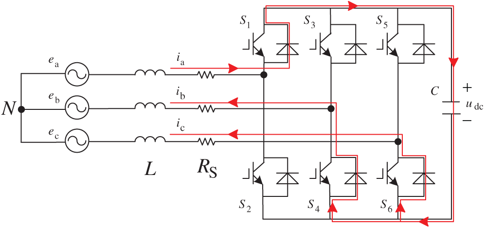
Figure 2: Schematic diagram of grid-connected current at the peak value of phase A

The circuit equation of phase A is as follows Eq. (13):

ea−icaRS−Ldicadt=0 (13)

The grid connection time of phase A is the peak time of a phase:

Ldicadt=0 (14)

According to Eq. (14), Eq. (13) can be simplified to Eq. (15), as shown in Fig. 3.

ea−icaRS=0 (15)

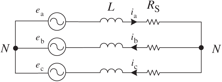
Figure 3: Simplified diagram of grid-connected current at the peak value of phase A

Therefore, the starting resistance can be determined by the following equation, where the peak value of and OCP is the level of overcurrent protection (OCP):

RS≥PeaOCP (16)

The transition process is the expected value of the DC side voltage when the SAPF works normally when the DC side voltage rises from u′dc. The expected value is set to 800 V in this system.

The SAPF control system adopts double closed-loop control with voltage on the outer loop and current on the inner loop. The outer voltage loop may be expressed as:

idc∗=kup(udc∗−udc)+kui∑(udc∗−udc)Ts (17)

Among them, u* dc is the expected value of DC voltage, kup is the proportional gain of the outer loop, and kui is the integral gain of the outer loop.

The inner current loop is expressed as:

uj=kjip(icj∗−icj)+kjii∑(icj∗−icj)Ts (18)

where i*cj is the expected current value, kjip is the proportional gain of the inner current loop, and kjii is the integral gain of the inner current loop.

When SAPF enters the transition process of uncontrolled rectification, the expected value of DC side voltage deviates greatly from the actual value. Under the regulation of the PI controller of the voltage outer loop, the output idc is larger, and the DC side voltage value rises rapidly, causing cause a certain overshoot and voltage impact. Under further regulation of idc by the PI controller of the current inner loop, the current icj rises rapidly and produces a certain overshoot, causesing a current impact.

4  Slow Start Strategy

From the previous analysis, we can see that the main causes of SAPF starting impulse are the rapid rise of DC voltage udc and current icj in the transition phase. Based on the above reasons, consider limiting the DC side voltage rise speed and current rise speed. Eq. (11) shows that the change rate of the voltage square can affect the current magnitude and current rising speed. Therefore, a rising curve based on the square of voltage can be designed to limit the rate of voltage rise and suppress the impact. Let the rising curve of the transition phase be Y, the transition time be ts, the expected value of the final DC side be u*dc = 800 V, the DC side voltage at the start of the transition phase is uncontrolled, and the voltage at the end of the rectifier phase is u′dc. Therefore, the rising curve Y can be set as the curve rising from 0 to Uf = u*dc−u′dc.

Fig. 4 shows two traditional rising curves, Y1 and Y2, respectively. Y2 is a piecewise function composed of Y21 and Y22. Eqs. (19) and (20) are their expressions, respectively, and Fig. 3 is the schematic diagram of Y1 and Y2 slopes [22,23].

Y1=Uftst (19)

{Y21=2Uftst20<t<ts/2Y22=Uf−2Ufts2(t−ts)2ts/2<t<ts (20)

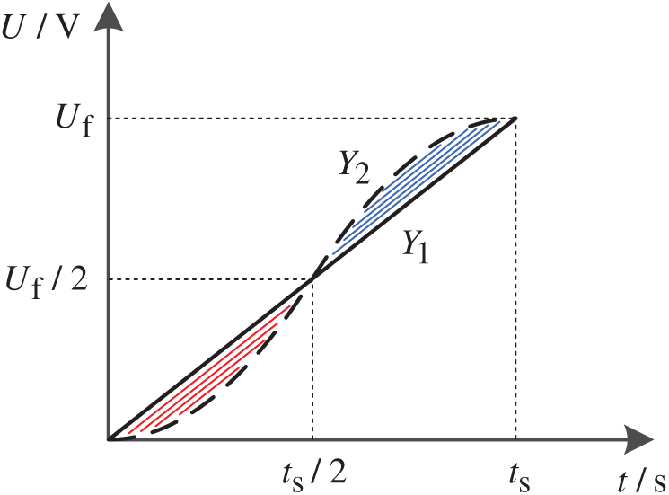
Figure 4: Schematic diagram of the rising curve in two traditional transition stages

It can be seen from Figs. 4, 5, and Eqs. (19) and (20) that the rising curves Y1 and Y2 in the transition stage have their advantages and disadvantages. In Eq. (7), Y1 and Y2 both improve the step response and restrain the impact to a certain extent. But when Y1 enters the transition phase, dudc/dt is a certain value and udc is 2.34E. According to Eq. (7), a step idc will be generated, and an impulse current will be generated under the action of PI control in the current inner loop. In the beginning, the instantaneous change rate of Y2 is 0, but according to Fig. 5, the instantaneous change rate between ts/4 and 3ts/4 exceeds Y1. According to Eq. (7), the instantaneous change rate will also affect the current. Therefore, there will be a certain current impact.

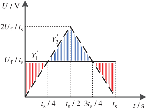
Figure 5: Schematic diagram of the slope of the rising curve in two traditional transition stages

From the above analysis, it may be noted that transition curves Y1 and Y2 have their advantages and disadvantages. Therefore, when combining them and taking the advantages of Y1 and Y2 to design the transition curve Y3 as shown in Fig. 6. Y3 is composed of three parts: Y31, Y32, and Y33. The expression is shown in Eq. (21). The instantaneous change rate of Y3 is shown in Eq. (22), where t2 = ts−t1.

{Y31=Uf2t1t2t20<t<t1Y32=Uft2t−Uft12t2t1<t<t2Y33=−Uf2t1t2(t−ts)2+Uft2<t<ts (21)

{Y31′=Uft1t2t0<t<t1Y32′=Uft2t1<t<t2Y33′=−Uft1t2(t−ts)t2<t<ts (22)

Eq. (22) represents the maximum instantaneous rate of change of Y3, which is also composed of three parts: Y31′ , Y32′ and Y33′ . The maximum value Y3′ is determined by t1. The smaller the t1 is, the smaller the starting impact is, which is helpful to restrain the impact, but the ts is prolonged correspondingly. The schematic diagram of Y3′ is shown in Fig. 7.

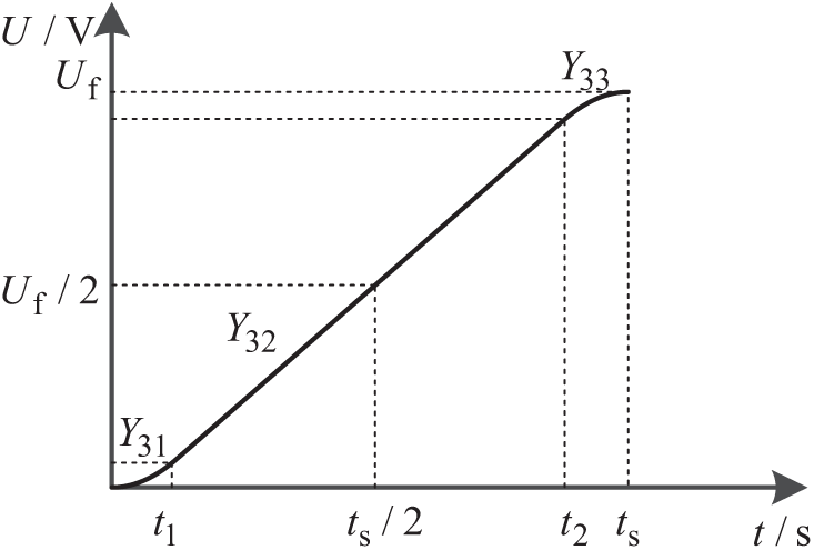
Figure 6: Schematic diagram of rising curve Y3 in the transition stage

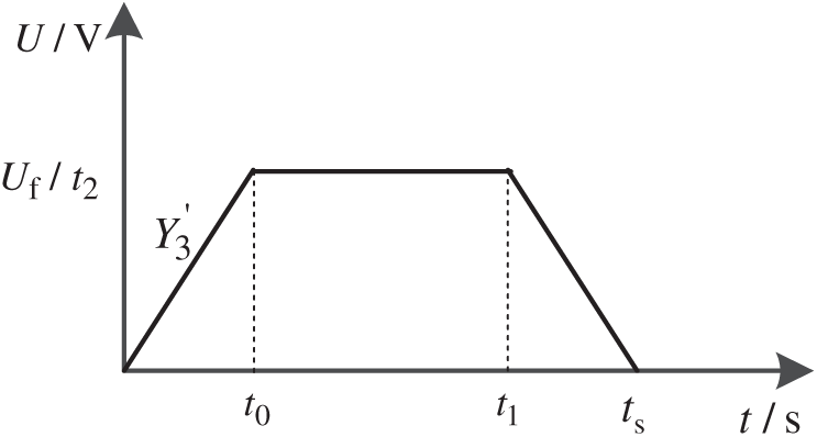
Figure 7: Diagram of instantaneous rate of change Y′3

However, the transition curve Y3 still has a disadvantage, that is, idc will increase with the increase of udc, which will lead to the gradual increase of impulse current and add instability factors to the system. According to the previous derivation, idc is related to udc2 , so the square of voltage is considered as the outer loop.

Therefore, the final transition phase rising curve combines the advantages of Y1 and Y2 and the mathematical relationship between idc and the design of the improved transition phase rising curve Y4 as shown in Fig. 8. When the starting time is set to t0, the expected voltage rises from 2.34E. Finally, the transition curve Y4 is designed as shown in Fig. 7, and the expression is shown in Eq. (23).

{Y41=(2.34E)20<t<t0Y42=Ufn2(t1−t0)(t2−t0)(t−t0)2t1<t<t2Y43=Ufn(t2−t0)(t−t0)−Ufn(t1−t0)2(t2−t0)t2<t<t3Y44=−Ufn2(t1−t0)(t2−t0)((t−t0)−ts)2+Ufnt3<t<ts (23)

where

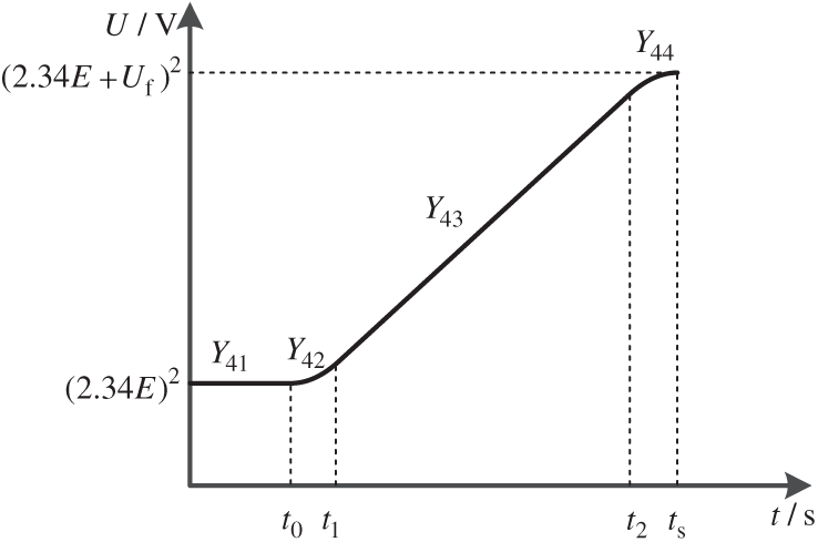
Figure 8: Schematic diagram of rising curve Y4 in the transition stage

Because of the square of the introduced voltage, Eq. (13) can be modified to Eq. (24) as follows [20]:

idc∗=kup(udc∗2−udc2)+kui∑(udc∗2−udc2)Ts=kup(udc∗+udc)(udc∗−udc)+kui∑(udc∗+udc)(udc∗−udc)Ts (24)

Let

{kup′=(udc∗+udc)kupkui′=(udc∗+udc)kui (25)

By changing the PI parameters, the rising curve based on the square of voltage can be changed back to the traditional rise curve to avoid the huge difference in the square of the voltage.

5  Simulation and Verification

To verify the improved transition phase rising curve proposed in this paper, a three-phase three-wire SAPF system model is built in the simulation software. The specific parameters of the system are shown in Tab. 1. The type of nonlinear load is the three-phase uncontrolled rectifier. Fig. 9 shows the nonlinear load current.

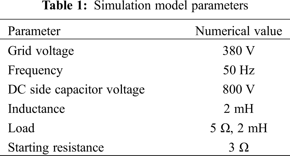
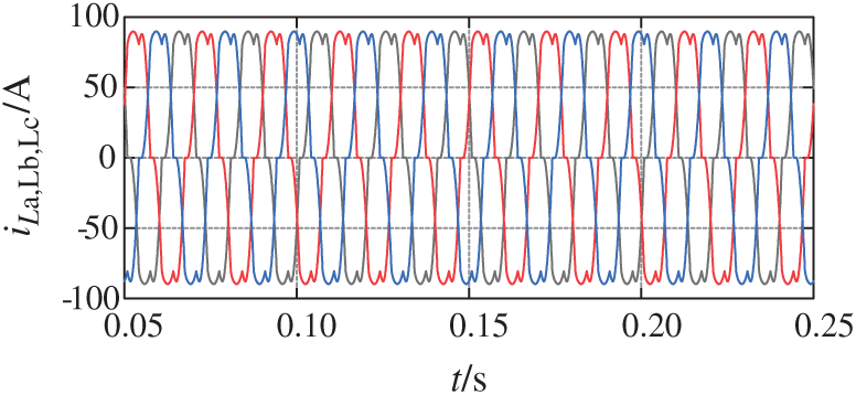
Figure 9: Nonlinear load current

Fig. 10 is the control block diagram of the SAPF system. Before 0.1S, the uncontrolled rectifier boost stage has been completed, and the voltage is stable at 2.34E. At 0.1S, the switch K1 is closed, and the system enters the transition stage. During the transition stage, the system does not compensate for the grid harmonics. When the DC side voltage rises steadily to the normal working voltage of 800 V, K2 is closed, and the system begins to compensate the grid harmonics, and SAPF begins to work. It works normally and the system starts up.

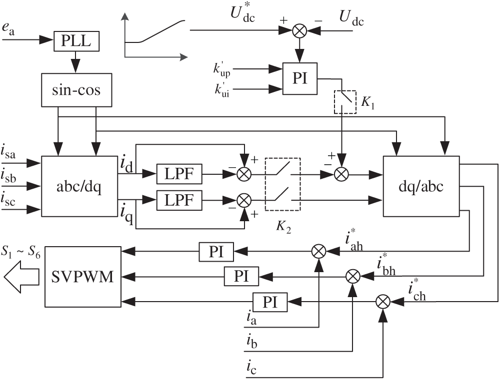
Figure 10: SAPF control block diagram

Fig. 11 shows that the starting strategy is not set, and the expected value of DC side voltage is 800 V. When the 0.1 s system is started, the actual value of DC side voltage is fast-tracking the expected value. The rising rate of DC side voltage is very high, resulting in the current surge as shown in Fig. 11a, and the DC side voltage overshoot, resulting in the voltage surge as shown in Fig. 11b. The impact current is more than four times the normal working current amplitude, and the impact voltage is nearly 200 V higher than the expected working voltage, which seriously threatens the safety of the system.

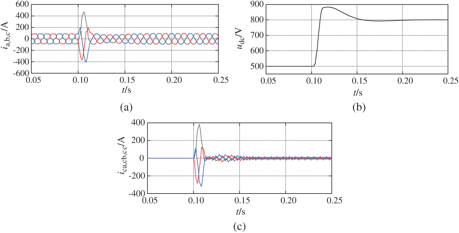
Figure 11: Voltage and current diagram when grid-connected starting strategy is not set. (a) Grid side current (ia, b, c). (b) DC side capacitor voltage (udc). (c) SAPF side current (ica, cb, cc)

Fig. 12 shows the voltage and current diagram using the traditional rising curve Y1 in the transition phase. Compared with Fig. 11, the impulse current and impulse voltage are basically suppressed. However, it can be seen from Figs. 12a and 12c that a large current impulse occurs at the moment when 0.1 s enters the transition phase. At the same time, it can be seen from Fig. 12b that the DC side voltage rises faster at the moment when 0.1 s enters the transition phase. This theoretical analysis is consistent with previous chapters.

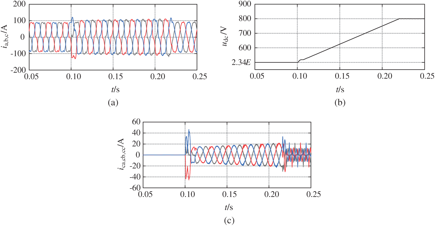
Figure 12: Voltage and current diagram with traditional starting strategy. (a) Grid side current (ia, b, c). (b) DC side capacitor voltage (udc). (c) SAPF side current (ica, cb, cc)

Fig. 13 is the voltage and current diagram when the transition phase rise curve Y3 is adopted. It can be seen from Figs. 13a and 13c that compared with Figs. 12a and 12c, the impulse current entering the transition phase is greatly suppressed, but the current gradually increases during the whole DC side voltage rise process, which increases the instability of the system to a certain extent. It can be seen from Fig. 13b that compared with Fig. 12b, the impulse current entering the transition phase is greatly suppressed Compared with the whole transition phase, the DC side voltage rises smoothly without overshoot and impact.

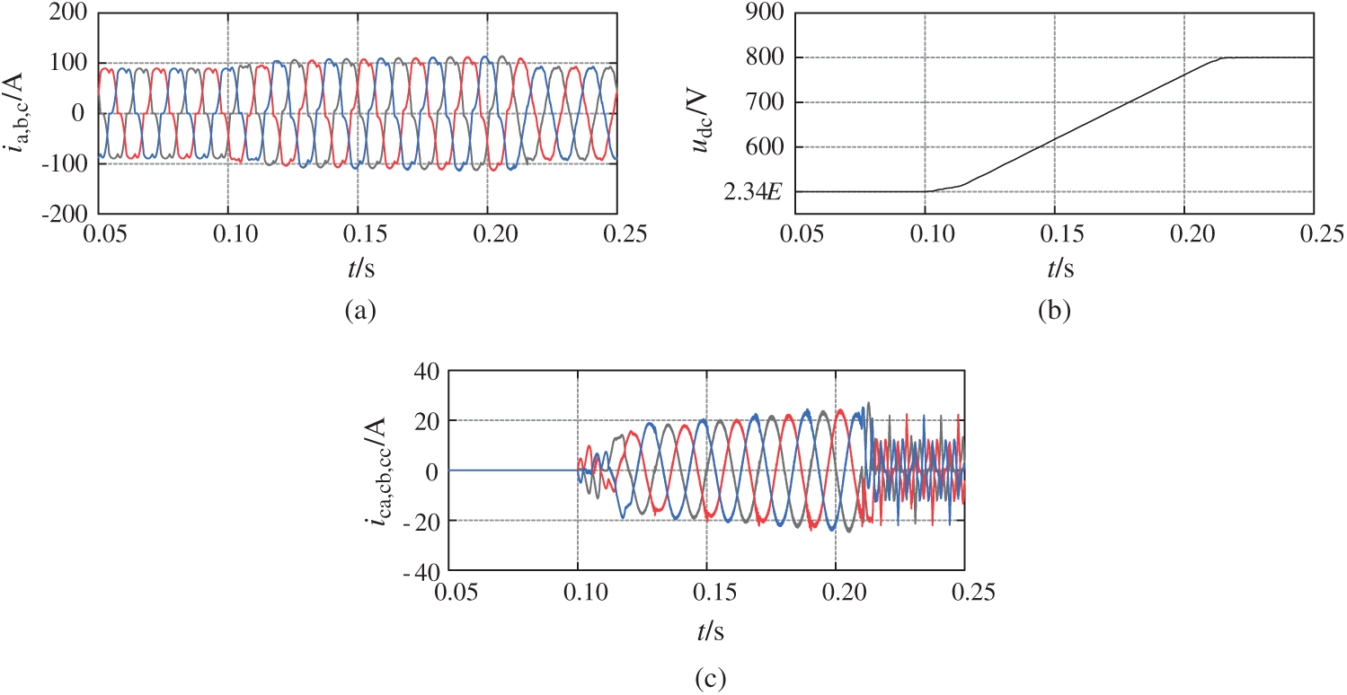
Figure 13: Voltage and current diagram with transition phase rise curve Y3. (a) Grid side current (ia, b, c). (b) DC side capacitor voltage (udc). (c) SAPF side current (ica, cb, cc)

Fig. 14 shows the voltage and current diagram of the improved transition phase rise curve Y4 based on voltage square and ts = 0.12 s proposed in this paper. It can be seen from Figs. 14a and 14c that compared with Fig. 13, the peak value of current in the whole transition phase is basically consistent, which effectively improves the stability and reliability of the system; during the whole starting process, the DC side voltage rises steadily without overshoot and impact.

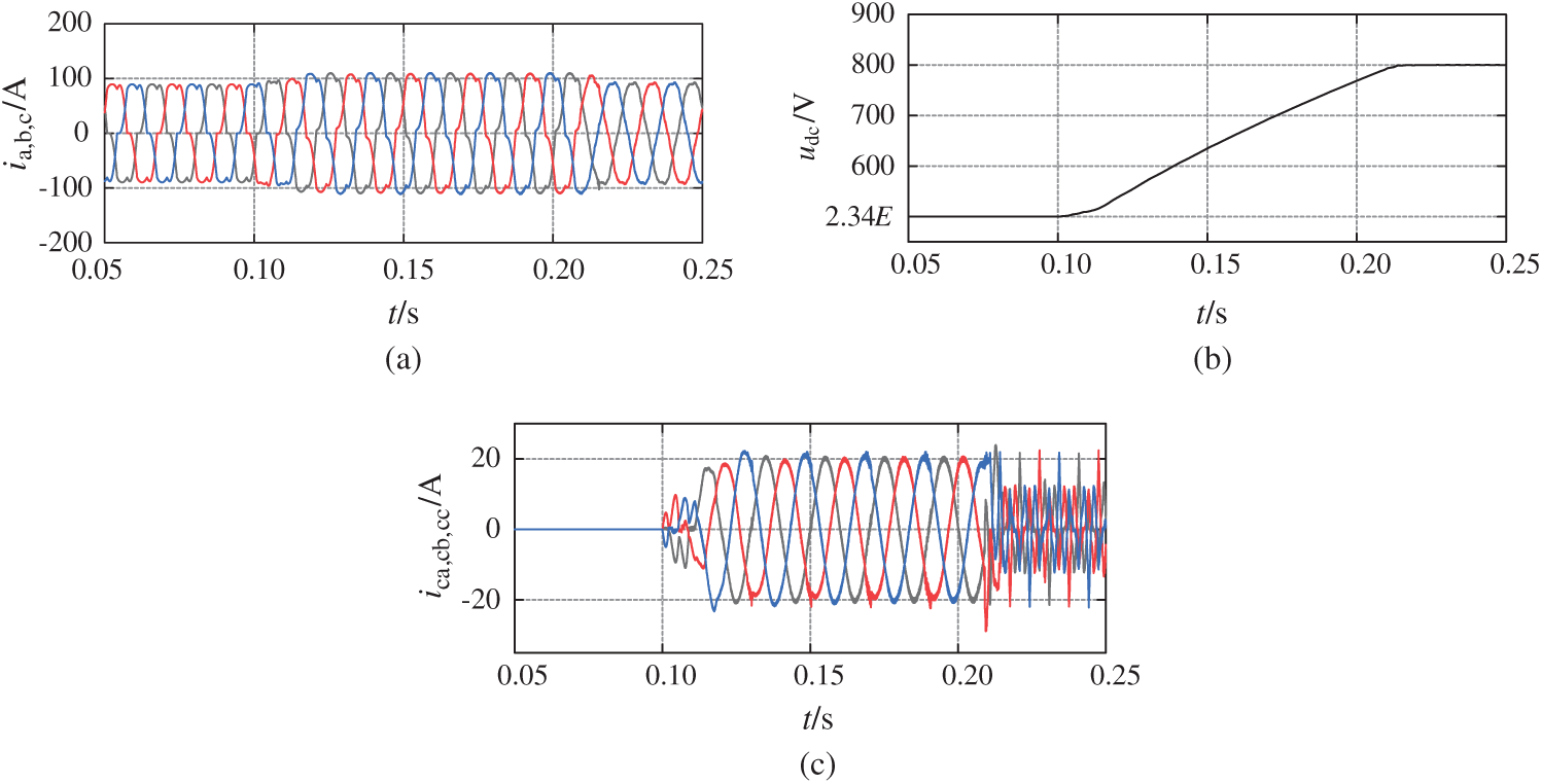
Figure 14: The improved transition phase rise curve Y4 and ts = 0.12 s voltage and current diagram based on voltage square are adopted. (a) Grid side current (ia, b, c). (b) DC side capacitor voltage (udc). (c) SAPF side current (ica, cb, cc)

Fig. 15 shows the voltage and current diagram when ts = 0.06 s. Compared with Fig. 14, the starting time is shortened, but the impact is increased, indicating that the greater the starting time is, the better the impact suppression effect is. However, the size of ts should be determined by comprehensive consideration to suit different systems.

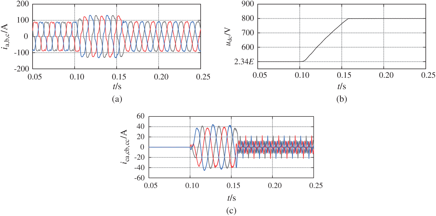
Figure 15: The improved transition phase rise curve Y4 and ts = 0.06 s voltage and current diagram based on voltage square are adopted. (a) Grid side current (ia, b, c). (b) DC side capacitor voltage (udc). (c) SAPF side current (ica, cb, cc)

Fig. 16 shows the change of total harmonic distortion (THD) value before and after the SAPF is put into operation. From the comparison between Figs. 11a and 11b, the THD value is reduced from 24.70% before compensation to 2.92% after compensation, which is in line with the national standard of less than 5%, indicating that the compensation effect of the SAPF system is good.

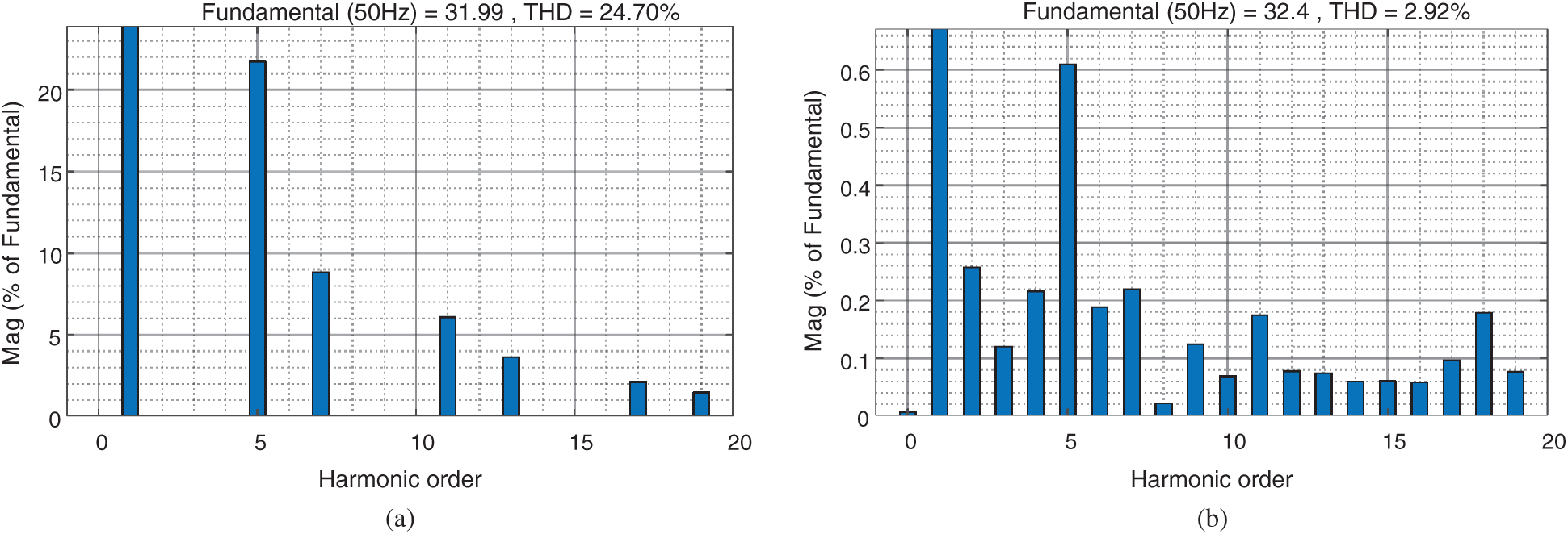
Figure 16: Comparison of THD before and after starting SAPF. (a) Before starting. (b) After starting

6  Conclusion

Aiming at the problem of impulse current and impulse voltage in the process of the grid-connected start-up of the SAPF system, the mathematical model of the DC side of SAPF is established, and the mathematical relationship between AC measured current and DC side voltage is obtained. According to the double closed-loop PI control system, the causes of impulse are analyzed, and an improved voltage rise curve in the transition phase based on the square of DC side voltage is proposed, which greatly inhibits grid-connected start-up The impact of starting the process. The SAPF system model is built in the simulation software to verify the effectiveness of the transition process rising curve proposed in this paper. Compared with the traditional rising curve, it greatly suppresses the voltage impulse and current impulse at the moment of entering the transition process. Compared with the square rising curve of non DC side voltage, the current of SAPF side will not rise with the rising of DC side voltage, which enhances the security and stability of the system. However, the length of the transition phase, ts, still needs to be further considered as the next key research direction.

Funding Statement: This work is supported by the National Natural Science Foundation of China under Grant 61863023.

Conflicts of Interest: The authors declare that they have no conflicts of interest to report regarding the present study.

This work is licensed under a Creative Commons Attribution 4.0 International License, which permits unrestricted use, distribution, and reproduction in any medium, provided the original work is properly cited.