Energy Engineering

DOI: 10.32604/EE.2021.017795

ARTICLE

Electricity Demand Time Series Forecasting Based on Empirical Mode Decomposition and Long Short-Term Memory

Saman Taheri1, Behnam Talebjedi2,* and Timo Laukkanen2

1Department of Mechanical and Energy Engineering, Purdue University, Indianapolis, USA
2Department of Mechanical Engineering, School of Engineering, Aalto University, Espoo, Finland
*Corresponding~Author: Behnam Talebjedi. Email: Behnam.talebjedi@aalto.fi
Received: 08 June 2021; Accepted: 29 July 2021

1  Introduction

Electric energy production and consumption have increased globally in recent years [1–3]; nevertheless, producing, transmitting, and delivering electrical energy are still complicated and expensive. To lower the cost of electricity generation and increase ability to satisfy the rising demand for electric energy, efficient grid management is critical [4–6]. Accordingly, effective grid management requires accurate demand forecasting [7–9]. Demand forecasting aids system operators in completing unit commitment and assessing power system stability. Given the fierce competition in the electricity market, load forecasting can provide valuable information for aggregators when participating in energy trading and dynamically managing electricity demand [10].

Many attempts have been made in the past to solve the challenges associated with load power forecasting (detailed reviews can be found in [11,12]). Inputs, outputs, time intervals, scale, data sample sizes, and error types have all been considered when classifying load forecasting approaches [13]. The accepted load forecasting approaches can be categorized as follows. Regression or/and multiple regression are still commonly used and effective for long-term (≥1 week to several years ahead) prediction, according to [14]. Machine-learning (ML) and time series (including the autoregressive moving average (ARMA) and autoregressive integrated moving average (ARIMA)) [15] are preferred for very short (≤1 h) and short-term (hours or days ahead) prediction. Meteorological data are the most commonly used independent variables, particularly incorporated in ML models [16]. In most instances, time series analysis and regressions depend solely on historical electricity results, with no exogenous variables introduced.

Although ARMA and ARIMA are versatile and simple models, they are linear in nature and therefore are restricted in performance when dealing with real-world data, which often exhibit non-linear and temporal patterns [17]. To deal with this uncertainty and variability problem, non-linear forecasting algorithms should be incorporated. In this regard, previous studies have highlighted ML models due to their high performance and accuracy [18]. Artificial neural networks (ANNs) [19,20], Regression-based models [21], support vector machine [22], extreme gradient boosting (XGBoost) [23], and deep learning are among the most popular ML algorithms used on the task of demand forecasting. A comprehensive review of learning-based models, their applications, and performance comparison can be found in [18].

Of all the ML algorithms in the field, deep neural network (DNN) algorithms provide better learning capability, mainly when dealing with data with non-linear behavior [24–26]. Compared to other ML algorithms, the better performance of DNN models is shown in several studies [27–29]. For example, Dedinec et al. [30] made up a deep neural network to anticipate the building electricity demand. Their results show an 8.6% improvement in mean absolute percentage error compared to shallow multilayered perceptron networks. Deep neural network networks, in essence, increase the strength of ANNs by deepening their layers through stacking several layers. Stacking different layers can be done differently by creating multiple classes of DNNs with different configurations and characteristics. Three major classes of DNNs are (I) autoencoders that are developed to learn features and reduce dimension of big datasets [31]; (II) convolutional neural networks, which are used for image recognition, classification, etc. [32]; and (III) long short-term memory (LSTM) units, which is capable of learning order dependence in sequence prediction problems [33].

LSTM has recently been the focus of increased attention for load forecasting problems as it can fit with highly complex and non-linear datasets. LSTM is tested against a publicly available dataset of residential meters in [34]. Results showed that LSTM outperforms rival ML algorithms in the challenge of short-term load forecasting for individual residential households. LSTM algorithm is used to train a dynamic model and generate predictions for impulsive loads in [35]. Marino et al. [36] explored two LSTM-based architectures: 1) regular LSTM and 2) LSTM-based Sequence to Sequence. Both approaches were tested on a benchmark data collection with one residential customer's electricity usage data. Multiple configurations of LSTM are discussed in [7], and the best architecture along with optimized hyperparameters are proposed for load forecasting. A hybrid load prediction model is built on LSTM and XGBoost algorithms in [37]. The learning procedure of LSTM in time series forecasting consists of extracting patterns from past observations to estimate the underlying temporal relationships. Nevertheless, in real-world situations, a single LSTM cannot guarantee accurate electricity load forecasts due to model under-fitting, misspecification, or overfitting, as discussed in [34].

Hybrid structures combining classical statistical methods and LSTMs have achieved important accuracy outcomes in a variety of fields [38]. These hybrid systems use error series modeling, ensembling, stacking, or signal processing to increase LSTM's performance. Khashei et al. [39,40], and Zhu et al. [41] suggested hybrid systems that produce the final prediction via joint modeling of time series and residuals. To improve the effectiveness of coping with instabilities, signal processing techniques such as empirical mode decomposition (EMD) is often used in combination with LSTM networks [42,43]. EMD may well be applied to non-linear and non-stationary processes since it is dependent on the local characteristic and temporal dependencies of the data. Zhang et al. [44] forecasted land surface temperature using LSTM coupled with signal empirical mode decomposition (EMD). Their findings indicated that when EMD and LSTM are combined, the hybrid combination outperforms a single LSTM configuration in terms of accuracy and robustness. EMD divides the original data into multiple stable sub-series, allowing it to be fed into an LSTM. Although the combination of EMD and deep learning methods for data series prediction has been widely studied in several fields, few studies have combined and used EMD and LSTM methods for demand forecasting. This study aims to improve LSTM architecture performance for electricity demand forecasting problems by proposing a hybrid system using EMD. Based on the above discussion, the major contributions of this paper can be summarized as follows:

•   A step-by-step framework is developed based on EMD to extract the intrinsic signals of electricity demand profiles (Section 2).

•   A hybrid demand forecasting model is proposed based on empirical mode decomposition and LSTM network in order to resolve the limitations of single LSTM, catch related uncertainties, and improve forecasting efficiency (Section 3).

•   A systematic analysis of parameters affecting demand forecasting results has been performed in Section 3. Multiple forecasting horizons (short, medium, and long-term), as well as various error functions (root mean squared error, mean absolute error, coefficient of determination, and mean absolute percentage error), are considered to evaluate the model accuracy. The proposed model is also compared with other state-of-the-art ML models such as XGBoost and logistic regression. To the best of our understanding, this is the first comprehensive study that considers various forecasting horizons and multiple accuracy metrics simultaneously (Section 4).

2  Mode Decomposition of Electricity Demand Profiles

In this section, the dataset used in this study is discussed, along with its characteristics and attributes. Then, data decomposition into several sub-series using the empirical mode decomposition (EMD) technique is explained.

2.1 Data Characteristics

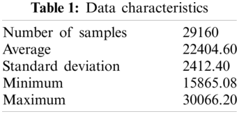
To help utilities quantify coincident peaks for demand forecasting purposes, the California Energy Commission provides four years of historical load data at a 1-hour resolution [45]. The dataset includes aggregated demand information for 2018, 2019, 2020, and 2021 (January−April), thereby containing 29,160 samples. Fig. 1 shows the demand profile between January and April of 2021. Fig. 2 illustrates the demand's probability density function, which provides additional context for the data's average and standard deviation. Tab. 1 summarizes the data characteristics and their associated attributes.

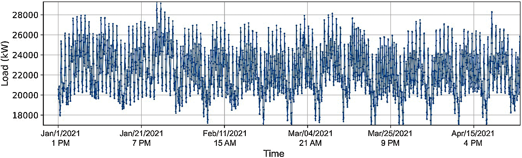
Figure 1: Demand profile between January and April of 2021

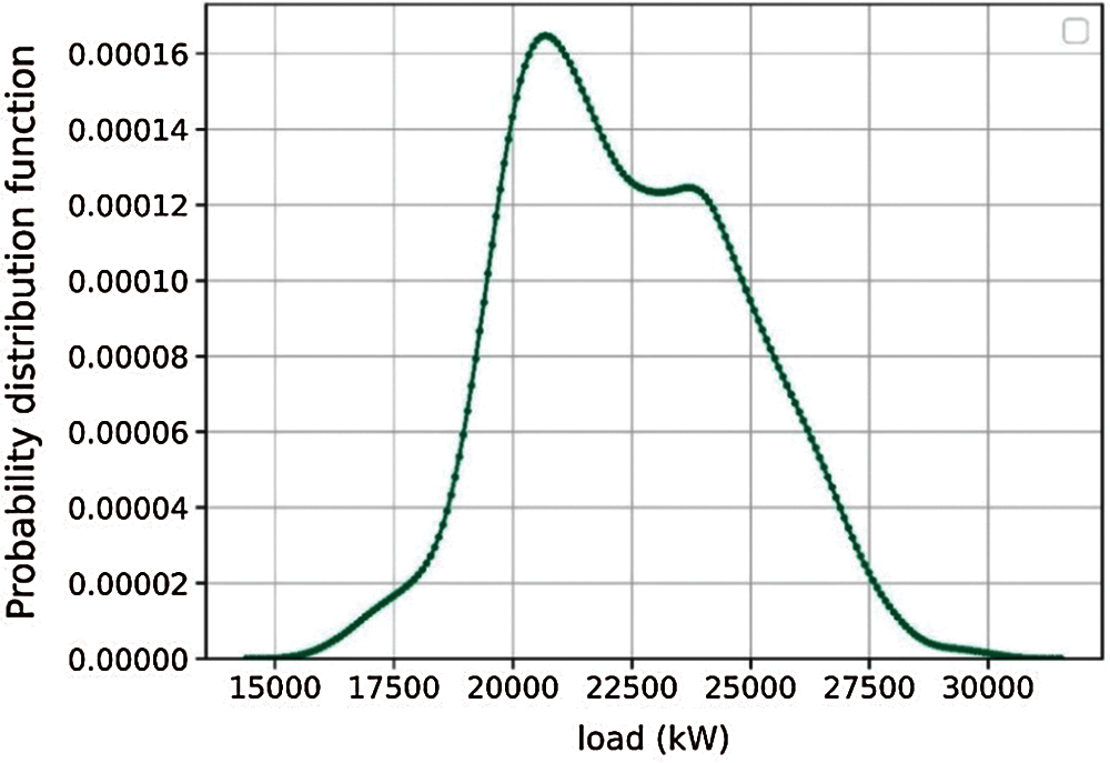
Figure 2: Demand's probability density function

2.2 Empirical Mode Decomposition

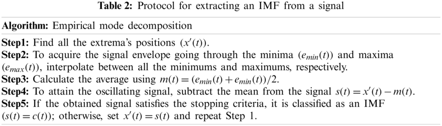
Empirical Mode Decomposition (EMD) is often desirable to decompose a signal, which is produced by multiple sources, in a way that approximates the contribution of each component. Fourier decomposition is a well-established mathematical technique for separating a signal into its components based on the frequency of fluctuations [46]. However, whenever a signal is nonstationary, such as when the signal mechanism varies with time, the right decomposition method to use is not obvious [47]. Empirical mode decomposition (EMD) is an alternative to Fourier decomposition in which the components of a signal are not constant in frequency over time, as would be the case if the signal generator is dynamic. EMD differs from theoretical decomposition, such as one relying on the Fourier Transform. As a result, it has several benefits when interacting with complex real-world signals, which are often nonstationary (i.e., not oscillating at the same frequency throughout time). EMD is mathematically expressed as follows:

x(t)=∑j=1J⁡cj(t)+rj(t)(1)

where x(t) is the original data, j denotes the index for the number of samples in the original dataset, cj(t) shows the jth intrinsic mode function (IMF), and rj(t) denote the residues. IMFs are constructed based on the local maxima, minima, and mean. Tab. 2 defines the protocol of extracting an IMF from a signal.

The step criterion (SC) for the final step is the gap in normalized squares of two consecutive iterations, which can be expressed as:

∑j=1J⁡||sj−1(t)−sj(t)||2sj−12(t)≤SC(2)

SC is usually placed empirically in the range (0.2–0.3). It is taken to be 0.25 in this study. Step 1–Step 5 is conducted for the representative dataset. Per Step 1, the extreme positions are calculated and shown in Fig. 3.

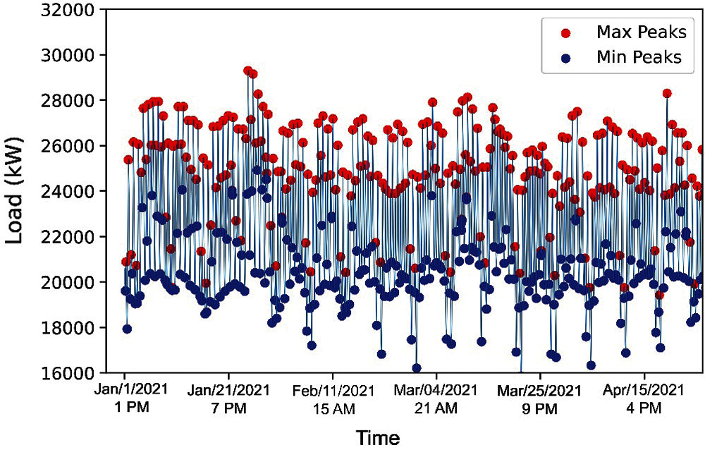
Figure 3: Positions of maximums and minimums associated with the representative dataset

For Step 2 and Step 3, the interpolation of maximum points, minimum points, and mean of those extrema envelopes are demonstrated in Fig. 4.

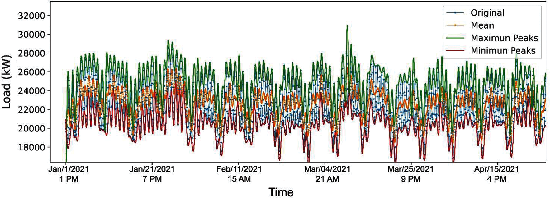
Figure 4: Minimum, maximum, and mean envelopes of the representative dataset

Next, oscillating signals are extracted based on the formula in Step 4 and then checked according to Step 5 to decide whether they have the potential to be regarded as IMFs. An IMF potential candidate oscillating signal is depicted in Fig. 5 to clarify the point.

The original dataset is decomposed into a variety of oscillatory modes or IMFs by repeating this method. Six IMFs are extracted from the original dataset, which is depicted in Fig. 6.

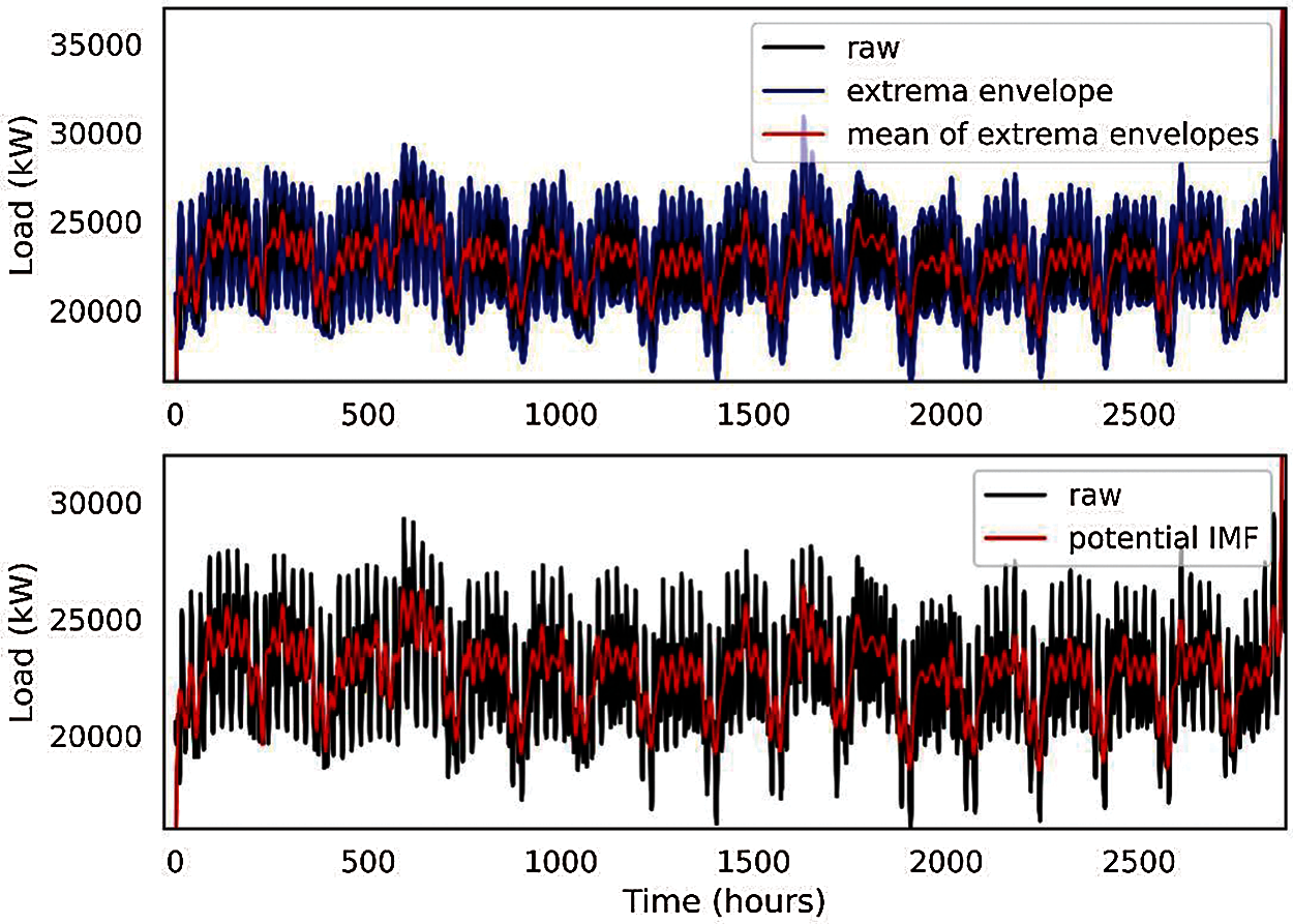
Figure 5: Potential IMF signal extracted from the original dataset

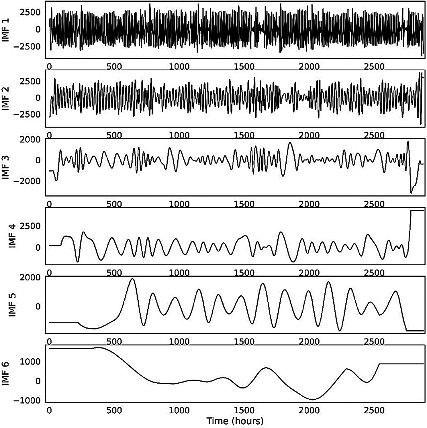
Figure 6: Intrinsic mode functions (IMFs) extracted from the historical load dataset

3  General Structure of the Proposed Method

In this section, the mathematical basis of the machine learning algorithms and the performance metrics used in the assessment process are presented. We then look at the general framework of the proposed method.

3.1 Long Short-Term Memory (LSTM)

A persistent limitation of classical neural networks is their inability to represent the temporal dependencies of operational datasets. To address this problem, recurrent neural networks (RNNs) are created. As shown in Fig. 7, a recursive framework enables RNNs to forecast a series of potential values using previously observable inputs while retaining knowledge over many time horizons.

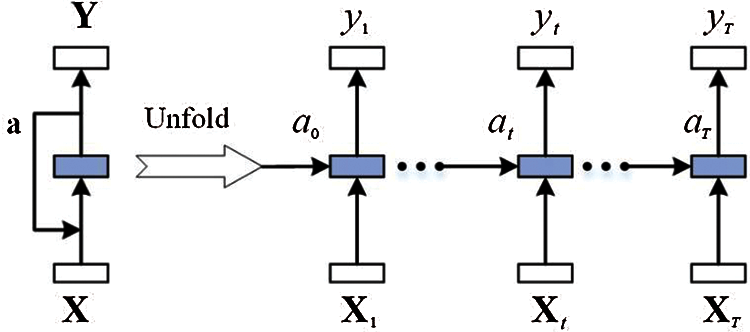
Figure 7: Schematic of a standard RNN structure (packed and unfolded in time)

RNNs are used to hope that utilizing historical data can help do more reliable load forecasting, even with a long-term time series. An activation function (a) determines the interaction between the output vector (Y) and the input vector (X). Typical RNNs, on the other hand, are unable to learn long-term temporal dependencies due to a phenomenon known as the vanishing gradients problem, which is discussed in detail in [48]. To address this problem, the LSTM unit is integrated into RNNs, converting them from normal to deep recurrent neural networks.

Hochreiter et al. presented LSTM as one of the deep learning strategies to increase the efficiency of standard RNNs in 1997 [49]. The training of LSTM is focused on the fact that it remembers previous states and can be prepared for tasks including state or memory recognition. Using this method, the LSTM network will solve problems related to gradient vanishing and bursting in standard RNN training phases. The LSTM, as seen in Fig. 8, is made up of memory cell mode blocks in which the flowed signal is controlled by an input gate, a forget gate, and an output gate. Each of these gates has its own set of computational relationships and functions, and the method of computing each vector at time t is shown below:

ft=σ(Wlflt+Wmfmt−1+bf)(3)

it=σ(Wlilt+Wmimt−1+bi)(4)

ot=σ(Wlolt+Wmomt−1+bo)(5)

at=tanh(Wlalt+Wmamt−1+ba)(6)

ct=ct−1∅ft+it∅at)(7)

where σ is the logistic sigmoid function, ft, it, ot, ct, and at, denotes forget gate, input gate, output gate, memory cell, and hidden vector, respectively. Wl∗=(Wlf+Wli+Wla+Wlo), and Wm∗=(Wmf+Wmi+Wma+Wmo), represent trainable weights of the respective gates while bf, bi, bo, and ba are output biases. Lastly, the operator ∅ defines the Hadamard product [50].

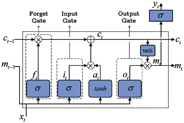
Figure 8: Principle architecture of the LSTM network

3.2 Performance Indices

Evaluating the performance of models using different metrics is an integral part of any forecasting. While there are multiple metrics, accuracy is mostly adopted to assess the quality of a model, including mean absolute error (MAE), root mean square error (RMSE), mean absolute percentage error (MAPE), and coefficient of determination (R2).

In this research, the model dataset is separated into two sections by proportions of P percent as the training set and (1-P) percent as the cross-validation (CV). Random subsampling is used to split the dataset into training and test sets. Data points are expected to be chosen from the same probability distribution. We next choose the P percent of these samples at random for the training set and the remaining (1-P) percent for the assessment test. We utilize different P values to test the generalizability of the ML models over different forecasting time periods. For example, P = 95 implies that 5 percent of the data (1,458 samples out of 29,160) is linked with CV; consequently, the relevant forecasting horizon is about (1,458/8,760) = 2 months.

MAE=1N∑i=1N⁡|ei|(8)

Root mean square error (RMSE)

RMSE=1N∑i=1N⁡ei2(9)

Mean absolute percentage error (MAPE)

MAPE=1N∑i=1N|eiyi|.100%(10)

R2=1−∑i=1N⁡ei2∑i=1N⁡(yi−y¯)2(11)

where N,yi, y^i, y¯ and ei denote the number of samples, observations, predictions, the mean of observations, and the error between the observations and the predictions, respectively. The MAE measures the mean of the error or bias, while the RMSE measures the standard deviation of the error or variance [51]. The smaller values of these metrics indicate the higher accuracy of the model. The major drawback of the MAE and RMSE is their inability to take into account the magnitude of observations. To solve this issue, the MAPE is introduced, measuring the mean of the absolute values of percentage errors. The MAPE values lower than 10% mean highly accurate forecasts, 11% to 20% mean good forecasts, 21% to 50% mean reasonable forecasts, and values more than 50% mean inaccurate forecasts [51]. The R2 measures the squared ratio of the residual sum to the total deviations sum with values between 0 and 1 in which values close to 1 imply higher accuracies and vice versa.

3.3 Decomposition-Based Long Short-Term Memory

Due to the uncertainty associated with load profiles, a single model is often insufficient to predict the electricity demand. Ensembling is a process of merging at least two ML algorithms to minimize bias/variance and maximize the learner's accuracy, precision, and robustness. Stacking is a heterogeneous ensembling that merges base learners in parallel, and then their predictions are fed as inputs to a meta-learner to form a new set of forecasts. Diversity of the base learners can be provided by using different learners, different hyper-parameter settings, different feature subsets, or different training sets. Herein, LSTM networks with the same hyper-parameters are adopted as base learners to exploit data deeply and learn order dependencies. However, the non-stationarity and stochasticity feature of meteorological variables still makes it challenging for LSTM networks to effectively recognize the pattern and provide high accuracy and robustness. To provide the requisite diversity and tackle the non-stationarity issue, two solutions are proposed in this paper based on mode decomposition and Dagging.

EMD decomposition technique is utilized to transform the non-stationary dataset into a series of relatively simple and stationary subsets. Therefore, a set of LSTM networks can be stacked in which each model only requires to focus on the frequency band components of a single subset, which can improve the overall performance of the stacked model. Moreover, Dagging technique is adapted to split the sizable non-stationary dataset into smaller equal-sized separate subsets and make it easier for the network to deal with the dataset's temporal dependencies. Therefore, a set of LSTM networks can be stacked in which each model only requires to focus on the corresponding subset, which can improve the overall performance of the stacked model. Fig. 9 illustrates the proposed stacking-based LSTM for accurate DLR forecasting based on mode decomposition and Dagging.

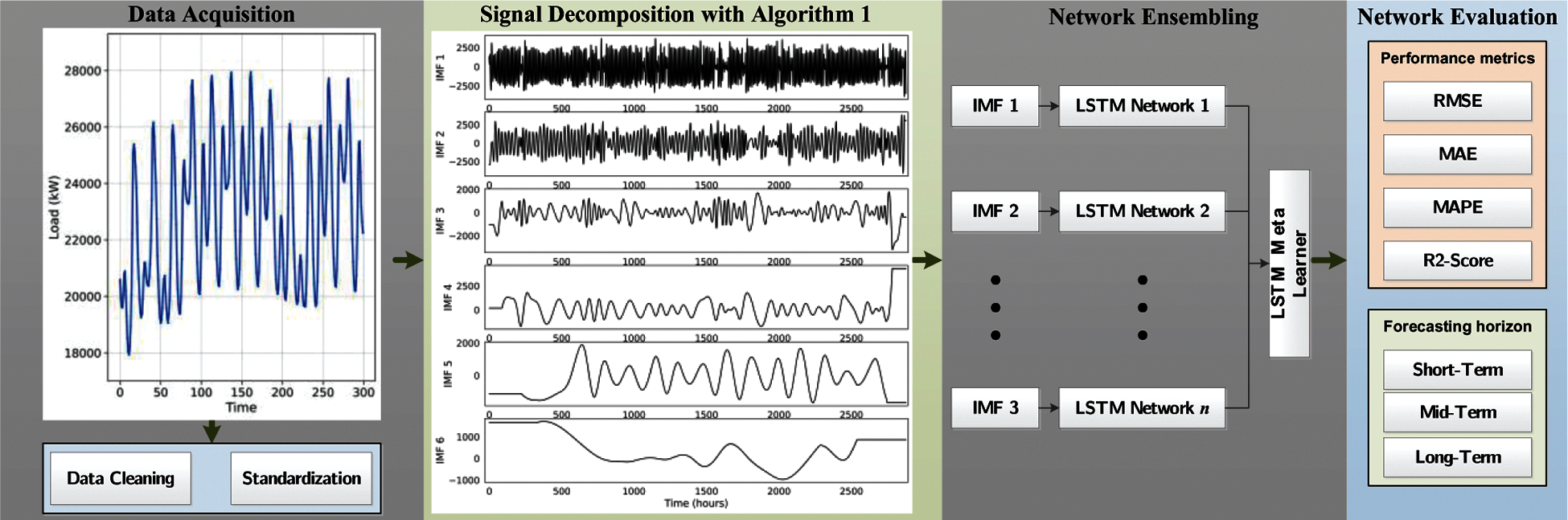
Figure 9: General structure of the proposed method

3.4 XGBoost Algorithm

XGBoost stands for extreme Gradient Boosting. Gradient boosting is a division of ML algorithms that works based on sequential learning techniques. This technique adds new models to improve the errors made by existing models. Models are added sequentially till no more improvements can be obtained. When all of the models are tuned, a highly accurate generalization model is obtained on the task. The hallmark of GB is its ability to strike the optimal balance between model sophistication and generalization performance. There are multiple GB architectures developed in previous studies. Compared to the other implementations of gradient boosting, XGBoost is a well-established and fast algorithm [52]. A detailed description of the XGBoost algorithm is out of the scope of this work, and interested readers are referred to [53] for further details.

3.5 Logistic Regression

Logistic regression (LR) was originally developed as a modified version of linear regression for classification problems. As opposed to linear regression, a logistic model computes a weighted total of the input features; however, instead of outputting the raw data like regression, it outputs a logarithm of the logistic value between zero and one. This gives LR the ability to fit with non-linear data. Here, we used an LR inspired by the study of [35].

4  Simulation Results

In this section, simulation results regarding the hybrid LSTM with Empirical Mode Decomposition (EMD), single LSTM, XGBoost algorithm, and logistic regression (LR) are provided. The studied data are the California ISO dataset which includes aggregated electricity demand from 2018 to 2020 and 2021 (January−April). Tab. 3 shows the model accuracy based on the model performance criterion discussed in chapter 2.4 for different time horizons. The studied time intervals for model evaluation are 24 h, 48 h, one week, and one month. The simulation results prove the superiority of the hybrid LSTM + EMD comparing to the single LSTM, LR, and XGBoost in terms of accuracy (model correlation coefficient and error). Results prove that in all prediction models, accuracy decreases from short-term to long-term prediction time horizons. For instance, in Hybrid LSTM + EMD, model root means squared increases from 278,76 to 423.22 and MAPE increases from 9.52 to 1,852, which correspond to 51% and 100% increase in RMSE and MAPE while the prediction time interval rises from 24 h to 1 month. On the other hand, the model determination coefficient also decreases 8.2% for Hybrid LSTM + EMD by increasing the prediction horizon from 24 h to 1 month. This fact is also true for other cases. For short term-load prediction (24 h) and long-term (1 month) electricity load prediction, the maximum determination coefficient (R2) of 92.2% and 84.5% can be accomplished by Hybrid LSTM + EMD, respectively. Tab. 4 shows the difference (changes) in model evaluation criterion for Hybrid LSTM + EMD for different time horizons with respect to the Single LSTM, LR, and XGBoost. It is clear from Tab. 4 that the XGBoost algorithm is the closest method to the Hybrid LSTM + EMD in terms of accuracy since there is the least amount of percentage changes of simulation error and correlation coefficient. The average changes in model RMSE compared to the Hybrid LSTM + EMD is XGBoost: −6.93, LR:−15.52, and single LSTM: −11.26 and the average changes in model determination coeffcinet is XGBoost: 4.58, LR: 26.72, and single LSTM: 22.72 where the minimum absolute changes in model error and determination coefficient is for XGBoost indicating it performs better compared to other machine learning algorithms. Fig. 10 visualizes the mean absolute percentage error of the different prediction methods, including the proposed Hybrid LSTM + EMD. In all cases, the MAPE of the proposed method is less than others, which shows that the Hybrid LSTM + EMD outperforms the other studied ML algorithms for electricity load prediction.

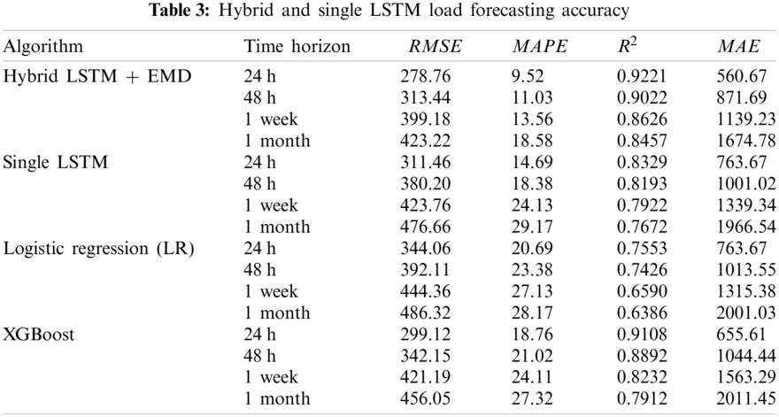
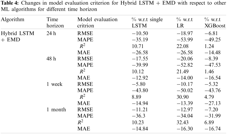
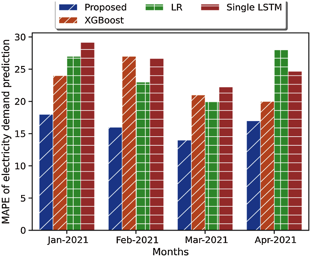
Figure 10: Mean absolute percentage error of different electricity load prediction methods (proposed method: Hybrid LSTM + EMD)

Fig. 11 illustrates the original (measured) electricity load data and predicted electricity load values for hybrid LSTM + EMD and single LSTM for different time intervals (40 to 700 h). The smaller the difference between the measured and predicted data, the higher the accuracy of the prediction and the model. As it is clear from the graphs, less simulation error can be found in hybrid LSTM since the target and predicted values are closer. Fig. 12 shows the original and predicted data for the proposed method and other state-of-the-art machine learning algorithms such as LR and XGBoost for 70 h time horizon. As it turns out, there is a greater correlation between the predicted data from the proposed method and the measured data, which indicates the higher accuracy of the proposed method than other machine learning algorithms.

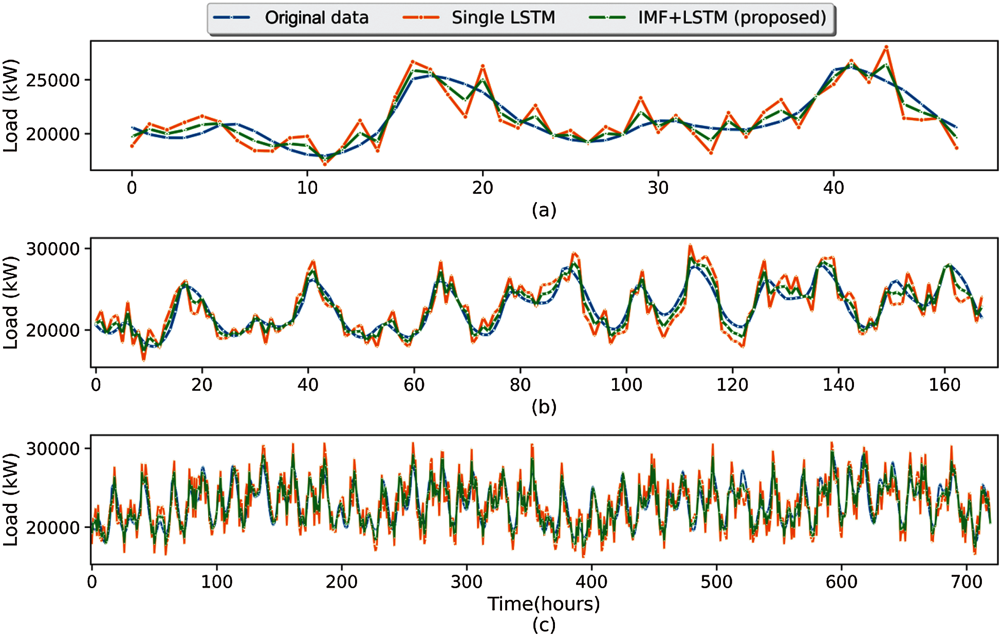
Figure 11: Original and predicted data of proposed LSTM + EMD and single LSTM algorithm for different time intervals: (a) 48 h; (b) 1 week; (c) 1 month

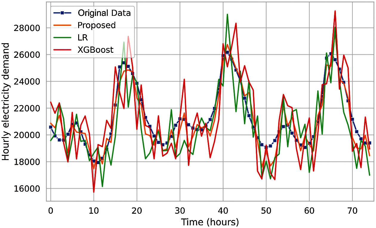
Figure 12: Original and predicted data of proposed LSTM + EMD and other state-of-the-art machine learning algorithms

5  Conclusion

Load forecasting is critical for a variety of applications in modern energy systems. Nonetheless, forecasting is a difficult task because electricity load profiles are tied with uncertain, non-linear, and non-stationary signals. To address these issues, long short-term memory (LSTM), a machine learning algorithm capable of learning temporal dependencies, has been extensively integrated into load forecasting in recent years. To overcome the shortcomings of single LSTM, capture relevant uncertainties, and increase forecasting performance, a hybrid demand forecasting model based on empirical mode decomposition and LSTM network (Hybrid LSTM + EMD) is proposed in this study. The model is intended to forecast California ISO aggregated electricity demand for the years 2018 to 2020, as well as 2021 (January to April). To assess the model's accuracy, multiple forecasting horizons (short, medium, and long-term) are regarded, as well as several error functions (root mean squared error, mean absolute error, coefficient of determination, and mean absolute percentage error). To test the efficiency of the proposed electricity load prediction techniques, the simulation findings are compared to other descent machine learning algorithms such as the XGBoost algorithm and Logistic regression (LR). Simulation findings show that the proposed Hybrid LSTM + EMD is superior to other machine learning methods for electricity load prediction, with correlation coefficients of 92% and 84% for short-term and long-term load prediction, respectively. In all cases (prediction approaches), the precision of the forecast model declines as the prediction horizon is extended. It can also be concluded that XGBoost outperforms single LSTM and LR in terms of overall performance and is more accurate for short-term prediction with the average determination coefficient of 91% for 24 h prediction horizon.

Funding Statement: The authors received no specific funding for this study.

Conflicts of Interest: The authors declare that they have no conflicts of interest to report regarding the present study.

This work is licensed under a Creative Commons Attribution 4.0 International License, which permits unrestricted use, distribution, and reproduction in any medium, provided the original work is properly cited.