Energy Engineering

DOI: 10.32604/EE.2022.016597

ARTICLE

Effect of Flow Field Geometry on Hydrodynamics of Flow in Redox Flow Battery

M. Narendra Kumar1,*, S. Manoj Kumar2, G. C. Vijayakumar1, K. Kadirgama3,4, M. Samykano5, Krishna Venkatesh1 and H. B. Murlidhara1

1Center for Incubation, Innovation Research and Consultancy (CIIRC), Jyothy Institute of Technology, Bangalore, 560082, Karnataka, India
2Department of Mechanical Engineering, Jyothy Institute of Technology, Bangalore, 560082, Karnataka, India
3Faculty of Mechanical and Automotive Engineering Technology, University Malaysia Pahang, Pahang, 26600, Malaysia
4Centre for Automotive Engineering, Universiti Malaysia Pahang, Pahang, 26600, Malaysia
5College of Engineering, Universiti Malaysia Pahang, Pahang, 26600, Malaysia
*Corresponding Author: M. Narendra Kumar. Email: narendra.kr@ciirc.jyothyit.ac.in; naru.sa@gmail.com
Received: 29 March 2021; Accepted: 09 July 2021

1  Introduction

In recent times there has been an increasing demand for non-conventional sources. Despite this, the fluctuating nature of nonconventional energy sources poses an immense challenge for far-reaching applications and efficient substitution of conventional sources. Thus, energy storage technology has a decisive role in delivering electric power from non-conventional sources. Of late, several technologies in energy storage have been proposed. These are characterized by distinct development levels and include pumped hydro, electrochemical, thermal, compressed air, flywheel, etc., among others [1]. Among several energy storage technologies, redox flow batteries (RFBs) have received considerable awareness. The autonomous extent of power and energy, prolonged durability, rapid sensitivity, scalability, flexibility, and decreased impact on the environment have resulted in making RFBs a reliable solution for aiding the generation of electricity from non-conventional sources. RFBs are considered as a promising contender for peak load saving [2] and being able to store larger electric power for medium and large scale uses in reasonably simple design [3,4]. Quite a lot of researchers are presently working on RFBs. They developed an all RFB that was simulated based on the first study on iron-chrome as a redox pair [5–7].

Earlier studies analyzed flow field design to attain uniform distribution with low ΔP, and minimize the mass transfer polarization of electrolyte to avoid solubility limits [8–10]. An all iron flow cell having a potentially low-cost advantage was also developed [11]. A semi-solid Li-flow battery was designed with an active slurry porous electrode via reaction chambers and showed that improvements in current density could be achieved [12]. An organic & inorganic RFB with quinine reactants in an aqueous electrolyte established higher current density with discharge capacity retention [13]. Some experimental and numerical studies on flow field details for RFBs were determined [14]. Flow cell stacks were developed for RFBs to enhance the limiting current and power densities [15–17]. Pressure drop ΔP losses in the stack, connected pipes, between stack and storage reservoirs need to be maintained at the lowest possible to reduce pumping power [18]. Several flow field designs were developed for fuel cell uses [19,20]. However, as mentioned earlier [21], the fundamental disparities between fuel cells and flow batteries necessitated a new perspective at flow field designs for RFBs applications.

A comparison study on the hydrodynamics of serpentine and interdigitated flow fields was performed [22]. Higher ΔP in a porous medium with a non-uniform flow of electrolyte resulted in adverse effects on the cell performance. The electrolyte needs to be uniformly distributed on its surface to reduce mass transfer polarization over the electrode’s entire surface [19,21]. Uniform flow of electrolyte was achieved at a higher flow rate that increased the cell capacity and increased pumping power, which reduces the efficiency of the stack. Therefore, it is necessary to manage an optimal flow rate that determines the balanced stack performance and capacity [23]. Parallel flow field (PFF) offered the lowest ΔP, but is affected by severe flow non-uniformities [24,25]. Also, under rib convection was insignificant with very little mass transfer by convection in the electrode [20,22].

A cell design with many slits at the inlet and outlet section provided a more uniform flow with the decrease in ΔP [26]. A bipolar plate with flow channel design to decrease ΔP, and to attain uniform flow distribution was suggested [27]. Later, they offered an interdigitated flow configuration for the cell [28]. They concluded that this configuration could increase the cell performance without much increase in ΔP appreciably. They also studied numerically various flow designs and concluded that as against traditional methods, the presence of flow distribution channels creates better flow uniformity along the electrode, and the introduction of channels inside it decreases the ΔP with very minimal net output power loss.

A review of RFBs on flow distribution, localized current distributions, limiting and maximum current densities, shunt currents and pressure distributions carried out [29] and concluded that to design advanced flow batteries and stacks for good electrochemical performance, much more experimental and modeling approaches was needed. Though several studies on the hydrodynamics of CSFF were reported, studies on the modified variations of CSFF were not much reported in the literature. In this study initial experiments were conducted on CSFF to determine the ΔP for different flow rates. Later, computational studies were carried out using in-house developed code based on FVM to check their agreement with experimental results. Results for pressure drop (ΔP) revealed that the deviation between the two was less than 5.1% (Fig. 3) for all the flow rates. This provided the impetus to explore other modified variations of CSFF with in-house developed code to study the effect of flow field geometry on hydrodynamics of flow in Redox Flow Battery (RFB).

2  Mathematical Modeling

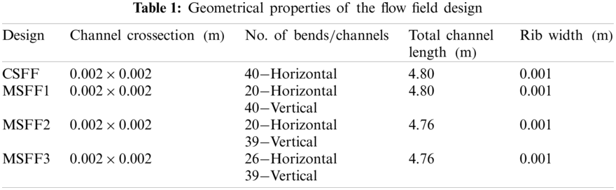
The physical system under investigation is described in Fig. 1 with its geometrical properties as shown in Table 1. The 3D geometry of computational domain consists of a flow field and the porous substrate with an active area of 0.0144 m2. In the simulations, the flow field and porous volumes for different designs were created using Solid Edge. A porous volume representing a fluid diffusion layer was placed below it with a specified permeability of 7.518e−11 m2 and porosity of 0.8. The common surface between the two volumes was considered as an internal surface without any flow resistance to fluid. A uniform inlet velocity, zero gauge pressure at the outlet, and no-slip condition on the walls of the flow domain were applied for all flow designs. The membrane does not influence the electrolyte flow across the membrane, only electron transfer occurs in this process. Since it does not affect the hydrodynamics of flow, the wall boundary condition was applied for the membrane.

Mass and momentum conservation for incompressible fluid flow are modeled as follows:

Mass conservation in flow

∇.(v→)=0 (1)

Momentum conservation in flow channel

∂(ρv→)∂t+∇.(ρv→v→)=−∇P+μ(∇v→+∇v→T)+ρg→+Sm (2)

For flow through channel, Sm=0

For flow through porous media,

Sm=−(μαvi⏟Viscousloss+C212ρ|v|vi⏟Inertialloss) (3)

Figure 1: Geometry of the flow field design (a) Conventional serpentine flow field (CSFF) (b) Modified serpentine flow field-1 (MSFF1) (c) Modified serpentine flow field-2 (MSFF2) (d) Modified serpentine flow field (MSFF2)

3  Numerical Simulations

To reveal the hydrodynamics of the flow fields, CFD analysis are conducted using in-house developed code based on FVM with 2nd order upwind differencing method for treating convective terms. The SIMPLE algorithm is used to couple the pressure and velocities on staggered grid arrangement with pressure being descriterised using 2nd order scheme. The porous substrate is modeled by the addition of source term to the momentum equation. This comprises of two components, a viscous loss term (first term) and an inertial loss term (the second term) in Eq. (3). Eqs. (1)–(3) were solved with relevant boundary conditions are solved using in-house developed code to ensure the convergence. Further, grid dependence test was conducted using four different grids with 1698316, 2244808, and 2597946, 2806912 cells. Except for case with least number of cells (306912), the solution obtained for the other grids was about the same. Therefore, simulations are carried out for 2597946 cells (Fig. 2).

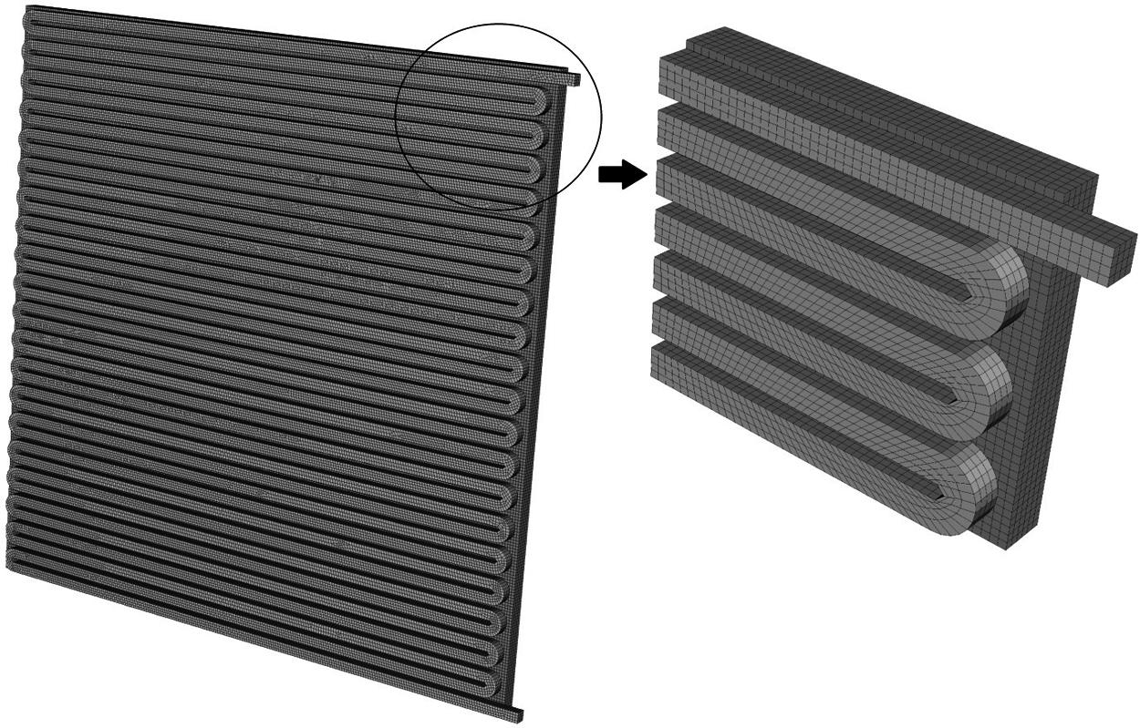
Figure 2: Typical grid of design model

4  Results & Discussion

In the present work, experimental (CSFF) and CFD analysis were conducted to reveal the hydrodynamics of flow in four different channels (CSFF, MSFF1, MSFF2 & MSFF3) for different flow rates (30--150 ml/min) using in-house developed code.

4.1 Experimental Results

Fig. 3 compares the pressure drop between experimental and CFD analysis for CSFF channel across the inlet and outlet section. The results of CFD analysis agree closely with the experimental data. The percentage deviation in pressure drop between the experimental and CFD analysis is of the order of about less than 5.1%. The pressure drop in the experimental is on higher side as compared with CFD results for all the flow rates due the unaccounted factors like surface roughness of channel, bends in pipe, pumping losses and friction, etc.

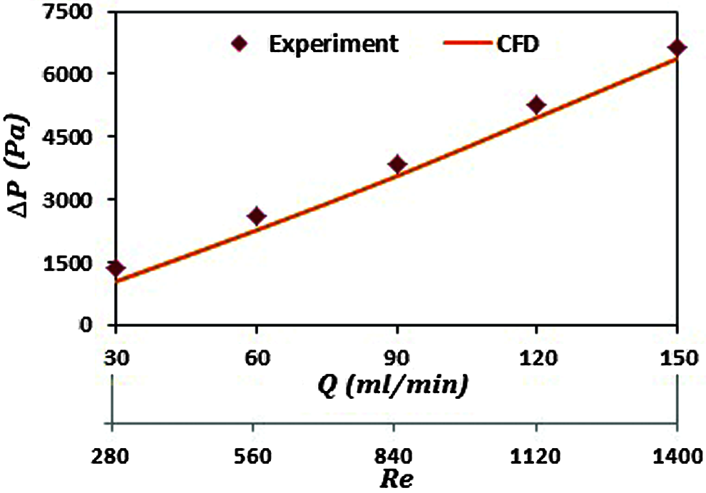
Figure 3: Variation of pressure drop against flow rates & Reynolds number for CSFF flow field

4.2 Simulation Results

Results from the simulations are presented in terms of Velocity distribution, Pressure distribution in Channel and porous substrate, Non dimensional Velocity distribution in Channel, Non dimensional Pressure distribution in porous substrate and Pressure drop for various flow rates for different channels. These are discussed in the proceeding sections.

4.2.1 Velocity Distribution in Channel and Porous Substrate

The velocity distribution in the channels of all four field configuration obtained from the simulation for flow rate of 150 mL/min is shown in Fig. 4. Fig. 4a, CSFF, most of the flow passes along the channel and is quite uniform across all channels, with higher velocity distribution at inlet and outlet region. In Fig. 4b (MSFF1), most of the flow passes through the channel and is quite uniform along flow channels in horizontal direction. When the flow changes to vertical direction, velocity distribution initially does present a non uniform flow due to gravity effect. As the flow stabilises it represents fairly uniform velocity distribution in succeeding channels. In Fig. 4c (MSFF2), most of the flow passes through the channel and is quite uniform along flow channels in horizontal direction. When flow changes to vertical direction, velocity distribution is disturbed due to gravity effect and does presents non uniform velocity distribution. With further change to horizontal direction, the flow represents fairly uniform velocity distribution. In Fig. 4d (MSFF3), similar trend is observed as in MSFF2 For all four field configuration shown in Fig. 4, higher velocity distribution is observed at inlet and outlet manifolds of the channel.

Figure 4: Comparison of velocity contours at mid plane of flow channel for different flow fields at Q=150 mL/min (a) Conventional serpentine flow field (CSFF) (b) Modified serpentine flow field-1 (MSFF1) (c) Modified serpentine flow field-2 (MSFF2) (d) Modified serpentine flow field-3 (MSFF3)

Fig. 5 depicts the distribution of velocity at the mid place of electrode for all four field configurations obtained from the simulation for flow rate of 150 mL/min. The velocity distribution in the porous substrate is two orders less in magnitude as compared to the flow through the channels. The velocity distribution shows a fairly uniform spread of fluid over the entire region of the electrode. Velocity penetration across the porous substrate is more in MSFF2 when compared with the other designs, which increases its wetting ability that is very important for the electrochemical reaction occurring in the porous substrate for effective electrochemical cell performance.

Figure 5: Comparison of velocity contours at mid plane of porous substrate for different flow fields at Q=150 mL/min (a) Conventional serpentine flow field (CSFF) (b) Modified serpentine flow field-1 (MSFF1) (c) Modified serpentine flow field-2 (MSFF2) (d) Modified serpentine flow field-3 (MSFF3)

Figure 6: Comparison of pressure contours at mid plane of flow channel for different flow fields at Q=150 mL/min (a) Conventional serpentine flow field (CSFF) (b) Modified serpentine flow field-1 (MSFF1) (c) Modified serpentine flow field-2 (MSFF2) (d) Modified serpentine flow field-3 (MSFF3)

4.2.2 Pressure Distribution in Channel and Porous Substrate

Fig. 6 shows the pressure distribution for four different flow field configurations achieved from simulation at flow rate of 150 mL/min. For CSFF, the ΔP across the cell is 6614.33 Pa with maximum pressure of 6821.44 Pa at inlet region and minimum pressures of 207.09 Pa at outlet region (Fig. 6a). For MSFF1, the ΔP across the cell is 5106.74 Pa with maximum pressure of 5317.56 Pa at inlet region and minimum pressures of 210.82 Pa at outlet region (Fig. 6b). For MSFF2, the ΔP across the cell is 3991.67 Pa with maximum pressure of 4202.22 Pa at inlet region and minimum pressures of 210.54 Pa at outlet region (Fig. 6c). For MSFF3, the ΔP across the cell is 4834.19 Pa with maximum pressure of 5044.83 Pa at inlet region and minimum pressures of 210.64 Pa at outlet region in l (Fig. 6d). From Fig. 6, it is observed that the pressure decreases continuously in value as the fluid passes the through subsequent channels from inlet region to outlet region. The ΔP across the cell is maximum for CSFF and minimum for MSFF2 design.

Figure 7: Comparison of pressure contours at mid plane of electrode for different flow fields at Q=150 ml/min (a) Conventional serpentine flow field (CSFF) (b) Modified serpentine flow field-1 (MSFF1) (c) Modified serpentine flow field-2 (MSFF2) (d) Modified serpentine flow field-3 (MSFF3)

Fig. 7 depicts the pressure contours at the mid plane of the porous substrate for four different flow field configurations at flow rate of 150 ml/min. For all these combinations, the pressure distribution in the porous substrate shows higher pressure across the inlet region and a lower pressure at the exit region.

4.2.3 Non Dimensional Velocity Distribution in Channel

Fig. 8 shows the distribution of non dimensional velocity along non dimensional Y coordinate for four different flow fields in horizontal flow channels. Velocity distribution depicts higher magnitude of about 0.65 in the first, about 0.45 in the last channel and a more settled uniform parabolic velocity distribution with lesser magnitude of about 0.25 in the succeeding channels in between (Fig. 8a). Similar trends were observed in MSFF1, MSFF2 & MAFF3 configurations for flow through the horizontal channels as shown in Figs. 8b–8d.

Figure 8: Comparison of velocities at mid of flow channel along Y coordinate for different flow fields at Vin=0.625 m/s & X=0.5 (a) Conventional serpentine flow field (CSFF) (b) Modified serpentine flow field-1 (MSFF1) (c) Modified serpentine flow field-2 (MSFF2) (d) Modified serpentine flow field-3 (MSFF3)

Fig. 9 shows the distribution of non dimensional velocity along non dimensional X coordinate for three different flow fields in vertical flow channels. In MSFF1, the Velocity distribution is minimum in magnitude in the first channel, subsequently increases in magnitude in the succeeding channels and reaches a maximum in the last channel (Fig. 9a). In MSFF2, the Velocity distribution is maximum in first vertical channel subsequently decrease in magnitude as it approaches the succeeding channels until the middle of the cell and increases in magnitude and reaches a maximum in the last channel (Fig. 9b). In MSFF3, similar trend was observed as in MSFF2 flow field configuration (Fig. 9c). Fig. 9 depicts a non uniform velocity distribution in all the configurations, primarily due to gravity effect in the channels, still presenting parabolic profile.

Figure 9: Comparison of velocities at mid of the channel along X coordinate for different flow fields at Vin=0.625 m/s & (a) Y=0.75 (b) Y=0.5 (c) Y=0.5

4.2.4 Non Dimensional Velocity Distribution in Porous Substrate

Fig. 10 shows the distribution of non dimensional velocity along non dimensional Y coordinate, along the mid plane of electrode for Q=150 ml/min & X=0.5 for four flow fields. In CSFF, the velocity distribution shows an oscillatory behaviour via mean amplitude of 0.006 over the entire the length (Fig. 10a). In MSFF1, the velocity distribution again represents the same pulsating nature with almost the same amplitude over first half of the length (Y=0.5). Further, for the remaining length, the velocity decreases to a very low value and essentially remains constant due the change in direction of the flow field (Fig. 10b). In MSFF2, the velocity distribution again shows oscillatory nature with the same mean magnitude (Y=0.3). As the flow changes to vertical direction, the velocity decrease to low magnitude and remains constant up to Y=0.7. Now, again, as the flow changes to horizontal position, the velocity again represents similar oscillations for the remaining length (Fig. 10c). In MSFF3, similar trends were observed as in MSFF2 (Fig. 10d). The velocity distribution in the electrode is two orders less in magnitude when compared with the velocity through the channel.

Figure 10: Comparison of velocities at mid plane of the electrode along Y coordinate for different flow fields at Vin=0.625 m/s & X=0.5 (a) Conventional serpentine flow field (CSFF) (b) Modified serpentine flow field-1 (MSFF1) (c) Modified serpentine flow field-2 (MSFF2) (d) Modified serpentine flow field-3 (MSFF3)

4.2.5 Non Dimensional Pressure in Porous Substrate

Fig. 11 shows the distribution of non dimensional pressure along non dimensional X and Y coordinates for four different configurations. For CSFF, the pressure distribution along X axis essentially remains constant in porous substrate as the flow is along the horizontal direction; along Y axis, the pressure varies linearly representing maxima at Y=0 towards the inlet section of the channel and minima at Y=1 towards exit section. In MSFF1, the pressure distribution remains constant up to about X=0.5 as the flow is in horizontal direction. Further, it starts decreasing along the length due to flow change in vertical direction. In MSFF2, the pressure distribution along X axis is maximum at X=0, decreases marginally up to X=0.2, remains essentially constant up to about X=0.8 and further decreases marginally. Along Y axis, the pressure decreases linearly as the flow is in horizontal direction up to Y=0.3, remains constant up to Y=0.7 as flow is now in vertical direction, further decreases linearly along length as flow changes to horizontal direction. In MSFF3, the same trend were observed as in MSFF2.

4.2.6 Pressure Drop for Various Flow Rates across Different Channels

Fig. 12a shows the variation of ΔP with respect to discharge across the inlet section and outlet section of the channel for different flow rates. The figure suggests that the ΔP increases as flow rate increases for all configurations. For all the flow rates under taken in this study, the ΔP is maxima for CSFF design, while it is minima for MSFF2 design. For CSFF, the ΔP is 1082.69 Pa for Q=30 mL/min. As Q increase to 60 mL/min, the relative value of ΔP increases by a margin of 53.36. As Q increase to 90 mL/min, the relative value of ΔP increases by 36.47, As Q further increase to 120 & 150 mL/min, its relative value increases by 28.26 and 22.27, respectively. For MSFF1, the ΔP is 808.26 Pa for Q=30 ml/min. As Q increase to 60 ml/min, the relative value of ΔP increases by margin of 52.91. With increase in Q to 90 ml/min, it increases by 38.38, As Q increase further to 120 & 150 mL/min, it increases by margin of 28.56 and 23.07 respectively, For MSFF2, the ΔP is 651.31Pa at Q=30 ml/min, with increase in Q to 60 ml/min, the relative value of ΔP increases by margin of 53.26, with increase Q to 90 ml/min, its value increases by 36.84, with further increase in Q to 120 & 150 ml/min, it increases by 28.01 and 23.23, respectively. For MSFF3, the ΔP is 801.72 Pa for Q=30 ml/min, the relative value of ΔP increases by margin of 53.13 with increase in Q to 60 ml/min, with increase in Q to 90 ml/min, its value increases by 36.69, for further increase Q to 120 & 150 ml/min, it increases by 27.84 and 22.55. This clearly shows that the percentage relative magnitude of ΔP decreases with increase in ΔP and Q.

Figure 11: Variation of non dimensional pressure at mid plane of electrode along (a) non dimensional X coordinate at Y=0.5, (b) non dimensional Y coordinate at X=0.5, for different flow fields

Figure 12: Variation of (a) pressure drop (b) % decrease in pressure drop in comparison with CSFF against flow rates & Reynolds number for different flow fields

Fig. 12b shows the % decrease in ΔP in comparison with CSFF design against flow rates & Reynolds number for three different flow fields. For MSFF1, at Q=30 ml/min, the % decrease in ΔP was 25.35; with increase in Q to 60 ml/min, the % decrease in ΔP was 26.06. For further increase in Q to 90, 120 & 150 ml/min, it was 23.21 22.88, respectively. For MSFF2, at Q=30 ml/min, the % decrease in ΔP was 39.84, as Q increases to 60 ml/min, it was 39.9 For further increase in Q to 90, 120 & 150 ml/min, it was 39.63. For MSFF3, the % decrease in ΔP was 25.95 for Q=30 ml/min with increase in Q to 60 ml/min, its value was 26.32 For further increase in Q to 90, 120 & 150 ml/min, its value was 26.07 26.49. Fig. 12b clearly suggests that the % decrease in ΔP is essentially constant for each of the modified designs in comparison with CSFF design for all flow rates and Reynolds number examined in this study.

5  Conclusion

From the experimental study of CSFF and CFD analysis for different flow fluid designs for different flow rates (30--150 ml/min), the following conclusions are drawn:

•   Development of the CFD in-house code based on FVM and its validation with the experimental results.

•   Experimental results and CFD analysis of CSFF design are in very close agreement within a percentage deviation in ΔP of less than 5.1%. The ΔP in the experimental study was on higher side, when compared with CFD results. The potential causes for it could be the unaccounted factors like surface roughness of the channel, bends in pipe, pumping losses and friction.

•   The ΔP across the inlet and outlet regions of the channel was maximum for CSFF design, while it was minimum for MSFF2 design. Percentage relative increase in magnitude of ΔP decreases with increase in Q for all the flow field designs. In comparison with the CSFF design, the percentage decrease in ΔP for all the modified designs was almost essentially constant with increase in Q, with an average magnitude of about 23.91% for MSFF1, 39.68 % for MSFF2 and 26.21% for MSFF3 design. Given that ΔP is one of the critical parameters in choosing RFBs, the recommended design would be MSFF2.

•   Comparing the relative magnitudes of flow velocity in channels and porous substrate for all the designs, the velocity distribution in the porous substrate was two orders lesser in magnitude as compared with flow in channel. Also by observing the velocity penetration across the porous substrate for all the designs, its penetration was found to be more in MSFF2 when compared to the other designs. This increases its wetting ability that is very important in terms of mass transfer over potential for electrochemical reaction happening in the porous substrate to achieve effective electrochemical cell performance.

From the results and discussion, it can be inferred that the MSFF2 design outperformed the other designs with minimum pressure drop and maximum wettability of porous substrate, which are very important for effective electrochemical cell performance.

Acknowledgement: The authors gratefully thank the Centre for Incubation, Innovation, Research and Consultancy (CIIRC), Jyothy Institute of Technology and Sri Sringeri Sharadha Peetam for supporting this research. K.Kadirgama would like to acknowledge Malaysia Minister of Higher Education for providing financial assistant under Fundamental Research Grant Scheme (FRGS) No. FRGS/1/2019/TK07/UMP/02/3 and Universiti Malaysia Pahang (UMP) under Grant No. RDU192207.

Funding Statement: The authors received no specific funding for the study.

Conflicts of Interest: The authors declare that they have no conflicts of interest to report regarding the present study.

This work is licensed under a Creative Commons Attribution 4.0 International License, which permits unrestricted use, distribution, and reproduction in any medium, provided the original work is properly cited.