| Energy Engineering |
DOI: 10.32604/EE.2022.017820
ARTICLE
A Novel Energy Lifting Approach Using J-Function and Flow Zone Indicator for Oil Fields
1School of Chemical and Energy Engineering, Universiti Teknologi Malaysia, Skudai, Johor, 81310, Malaysia
2School of Energy, Geoscience, Infrastructure and Society, Heriot-Watt University Malaysia, Wilayah Persekutuan Putrajaya, 62200, Malaysia
*Corresponding Author: M. N. Tarhuni. Email: motr_2008@yahoo.com
Received: 09 June 2021; Accepted: 19 August 2021
Abstract: The X field is located in the southwestern part of block NX89 of Kentan Basin in Libya. This field is produced from Hailan multilayer consolidated sandstone with moderate rock property and a relatively low energy supplying. The reserve of subsurface energy sources is declining with years. Therefore, techniques were combined to achieve the energy optimization and increase hydrocarbon recovery. In order to understand the subsurface formation of the reservoir and facilitate oil production, global hydraulic element technique was used to quantify the reservoir rock types. In addition, stratigraphic modified Lorenz plot was used for reservoir layering. Reservoir heterogeneity was identified using stratigraphic modified Lorenz plot and Dykstra-Parsons coefficient. Leverett J-function was used to average the 13 capillary pressure curves into four main curves to represent the whole reservoir based on flow zone indicator values. Capillary pressure was calculated and plotted with normalized water saturation; a single average curve was defined to represent the rest of the curves. Water saturation was calculated using single and multiple J-functions and compared with the available logs. With multiple J-functions, the matching results were good for both high and low-quality layers, whereas using a single J-function, the match was poor, especially for low FZI layers such as H4c and H6a. Four rock types were identified for this reservoir ranging from medium to good reservoir quality and six different layers were obtained. The reservoir was heterogeneous with a Lorenz coefficient value of approximately 0.72 and a Dykstra-Parsons value of 0.70. All approaches used in this paper were validated and showed improved hydrocarbon recovery factor.
Keywords: Energy lifting; special core analysis; flow zone indicator; reservoir heterogeneity; water saturation; Leverett J-function
| Nomenclature | |
| Interfacial Tension | |
| Wetting Contact Angle | |
| J(Sw) | J-function, Dimensionless |
| Pc | Capillary Pressure, psi |
| Vk | Dykstra-Parsons |
| Swi | Initial Water Saturation, % |
| k | Air Permeability, md |
| Porosity, % | |
| Lc | Lorenz coefficient |
| Ka | Arithmetic Average |
| kh | Harmonic Average |
| Swn | Normalized Water Saturation, % |
| Sirr | Irreducible Water Saturation, % |
| Sw | Total Water Saturation, % |
| J* | Lithology Index |
| Pore Size Distribution Index | |
| a, b | Coefficients |
The success of several energy engineering operations is highly dependent on petrophysical rock typing [1]. Two techniques are used in the rock selection for modeling and energy studies: these techniques are known as routinely defined rock types Routine Core Analysis (RCAL) and Special Core Analysis (SCAL). Identifying regions with similar features (definable and statistically predictable properties) for better characterization and modeling of reservoirs is known as rock typing [2]. In comparison, special core analysis involves more fluid flow laboratory experiments and energy measurements, including: two-phase flow properties, capillary pressure, wettability, and relative permeability [3–5]. Generally, any meaningful classification that differentiates and describes the reservoir based on special characteristics might be attributed to rock typing [6,7].
The petrophysical rock typing approach has been widely applied in drilling to predict the high fluid loss zones and in production to locate perforations, define potential high energy zones, and design diversion systems in acidizing [8,9]. Petrophysical rock typing has been used in many energy studies (e.g., net-pay cut-off definition) [10] and predicting the permeability of un-cored reservoirs [11–13]. However, the most significant energy engineering applications that can directly impact the simulation models output and their reliability are representative sample selection for SCAL tests by reducing the number of required representative samples [1,4,14,15] and determining saturation functions for static/dynamic reservoir modeling [2].
Porosity and permeability are considered as the main reservoir quality controlling factors in reservoir characterization and energy processes. The hydrocarbon storage capacity of a reservoir is a function of porosity, whereas reservoir deliverability is a function of permeability [16]. Lithological, petrographic, and petrophysical data are required to identify, describe, and rank the reservoir flow units and its energy sources. Ideally, this kind of data should be evaluated in combination to detect and interpret the correspondences between them [17]. Successful water injection plans and accurate energy characterization require a better understanding of reservoir quality, heterogeneity and energy potential [18]. Therefore, this paper will broadly address these issues.
Building a robust reservoir dynamic model relies on reservoir characterization and energy management as well as reliable predictions. In order to proceed to SCAL analysis such as Pc curves, it is vital to define rock types, reservoir quality, zonation, and heterogeneity through conventional core analysis and relate it to the geological facies and SCAL interpretation [19–22].
One of the most crucial pieces of information that can be obtained from SCAL is capillary pressure. This capillary phenomenon can occur when two or more immiscible fluids are present in the rock pores. Due to the interfacial tension (IFT) and energy differences between the two phases, the pressure difference across the interface is generated. Capillary forces cause the fluid to retain in the pore space against gravity forces, and it can be simply defined as the difference between the wetting and non-wetting phases. It represents the interaction between rock and fluid, which is affected by many factors, including interfacial tension, wettability, pore geometry, size, and distribution. Pc curves can be determined under two separate processes: drainage and imbibition [23–27].
The flow of several phases occurs in a diverse range of industrial processes, particularly in the petroleum industry where mixtures of oil and water are transported through pipelines over long distances. Multiphase flow which is also known as simultaneous flow is important in energy-related industries and applications. Two-phase flow is a form of multi-phase flow that can occur in different states such as solid-liquid, liquid-liquid, gas-solid, and gas-liquid flows. Immiscible hydrocarbon flow such as oil and water is crucial in oil recovery mechanisms that can be considered as a liquid-liquid flow. In the presence of multiphase fluids, the dimensionless Leverett J-function describes the water saturation of an oil reservoir based on capillary pressure forces. This function synthesizes the fluid IFT, wettability, porosity, and permeability to represent the characteristics of the reservoir, hence maximize its energy potential and hydrocarbon recovery. It is an efficient method to analyze data on capillary pressure [28–33].
Water saturation is a crucial element in determining oil saturation. Average water saturation is usually identified from capillary pressure data for a homogenous reservoir. On the other hand, in a stratified reservoir, obtaining an accurate value would be more difficult as the water saturation depends on permeability. If the permeability varies from one side to another within the reservoir, water saturation might be a complex function of the reservoir's height. It can be obtained from capillary pressure data (Leverett J-function) and arithmetic or geometric averaging of the permeability. Once the water saturation is obtained, oil saturation can be determined using a mathematical conversion [34,35].
Due to reservoir heterogeneity and subsurface energy variation, there is no single Pc curve can be used to represent the whole reservoir. Therefore, capillary pressure curves are normalized using Leverett dimensionless J-function to convert Pc curves into a single curve that can be considered for a unique rock type. Leverett J-function accounts for the difference in porosity, permeability, interfacial tension (σ), and contact angle (θ). As capillary pressure depends on pore size radius, Leverett J-function can also be used to determine pore sizes for rocks of uniform properties. In complex reservoirs, as the water saturation is a function of capillary pressure height and rock properties, Leverett J-function, J(Sw) works much better than normal Pc(Sw) [23,24,34,36–38]. This research is useful in reducing the simulation complexity as well as the uncertainty associated with reservoir modelling. In addition, the methodology and findings of this paper can be applied to other fields to identify various rock types and characterize them in order to create simulation properties with the power to predict the future reservoir behavior. Knowledge about these fracture is also significant in reservoir management and well performance.
2.1 Rock Types Identification Using GHE
There are various flow unit determination methods in the literature. Each of them has distinct advantages, limitations, and results. These approaches may include Hydraulic Flow Unit (FHU) and Flow Zone Indicator (FZI) [11,39–41], Discrete Rock Type (DRT) [42], Winland and Pittman [43–45], Lucia carbonate rock typing [46–48], Global Hydraulic Element (GHE) [14,49–51], Modified Flow Zone Indicator (MFZI) [52], Petrophysical Dynamic Rock Type (PDRT), Petrophysical Static Rock Type (PSRT), Petrophysical Static Rock Type Indicator (PSRTI) [1,4,53,54], and Stratigraphic Modified Lorenz Plot (SMLP) [55–60]. In this paper, selecting the right method to be applied for the X Field was dependent on the most accurate method and data availability and accessibility.
GHE has been determined for Well X1 (Hailan formation) based on core porosity and permeability. Quality control (QC) was conducted to ensure a clean dataset was available for the analysis process. The reservoir quality index (RQI) and Normalized Porosity Index (NPI) or (Φz) were calculated using core data Eqs. (1) and (2) were used to calculate RQI and Φz, respectively,
where, k is the rock permeability, and
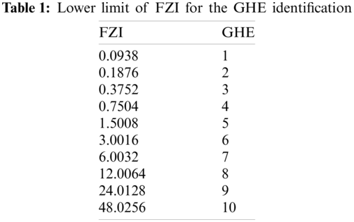
FZI was then calculated using Eq. (3) which was used to determine the GHEs using the boundaries in Table 1.
The unit of RQI and FZI is (μm).
Generally, the GHEs are ranging from 1 to 10, which indicates the quality of the reservoir. GHE of 1 indicates poor reservoir quality with the lowest FZI boundary of 0.0938 μm [49]. Whereas a GHE of 10 shows the best reservoir quality with the highest FZI of 48 μm.
SMLP is a powerful technique to identify reservoir layers. In SMLP, reservoir zones are characterized by straight lines; the line's slope illustrates the reservoir's overall quality. With this plot, it is possible to divide the reservoir into different zones by observing the change in the slope. The steeper the slope, the faster the rate of flow and the better the reservoir quality. In contrast, horizontal trends illustrate little or no flow and poor reservoir properties.
2.3 Classifications of Reservoir Heterogeneity
Several methods might be used to classify the reservoir heterogeneity, including (Lc), which is sorting the permeability from low to high order and then constructing Ordered Lorenz Plot (OLP). The area under the curve and above the 45° line was then calculated to represent the reservoir heterogeneity. The Lc value ranges from 0 to 1; the latter represents the highest degree of heterogeneity, and the closer to 0, the more homogeneous the reservoir is [23]. Lc can also be calculated using the following correlation, which mainly depends on obtaining the Dykstra-Parsons (Vk) and substituting the value in Eq. (4) [61–64].
where,
Ka is the arithmetic average, and kh is the harmonic average.
2.4 Conversion of Pc Laboratory into Pc at Reservoir Condition
For X1-NX89, capillary pressure curves were generated in the laboratory using a mercury pressure cell, and the fluid system was Air-Water (Brine). Generated data using these techniques will not be directly compared to each other or to reservoir conditions; therefore, a conversion process from laboratory to reservoir condition must occur. To initialize the static model, it is common to use Air-Brine derived capillary pressure curves, taking into account a vital assumption that Air-Brine Pc curves can be converted into equivalent oil-water drainage capillary pressure curves using Eq. (6) as follows:
where subscript L refers to the laboratory (Hg-air) and R to reservoir (oil-water) fluids, σ is the interfacial tension between the two fluids, and θ is the contact angle. Once this conversion has been completed, capillary pressure curves at reservoir conditions can be plotted with water saturation.
2.5 Normalized Water Saturation Calculation
Normalized water saturation Swn was calculated using Eq. (7) as follows:
where Swn is the normalized water saturation, Sw is the water saturation, and Sirr is the irreducible water saturation. Once Swn is obtained, a linear multi-regression method, i.e., a plot between Pc at reservoir condition and normalized water saturation, was used to obtain the lithology index (J*) and pore size distribution index (λ). A regression quality check has been made before proceeding further to confirm the validity of the obtained results. This quality check was done by plotting (Sirr) vs. (Sw) at a selected Pc value. If a unit slope is obtained with R2 value close to 1 or at least greater than 0.8, then the regression is good, and the value of (J*) and (λ) can be used for further analysis.
2.7 Leverett J-Function and Average Capillary Pressure Curves
It is well known that capillary pressure curves are obtained from small rock samples, which can only represent a small part of the reservoir. Therefore, it is vital to combine all capillary pressure data to classify any particular reservoir. Leverett [65] proposed a general equation that can be used to combine and average capillary pressure curves as follows:
where J(Sw) is Leverett J-function, Pc is capillary pressure (psi),
2.8 Classification of Average Capillary Pressure Curves Using (FZI)
In this case, for X01-NX89, all Pc curves were processed by J-function to simplify them into a single monotonic curve that represents each rock type. This function's fitting trend was power rather than exponential or polynomial, which can be done throughout an investigation of the capillary pressure relation. Besides, Eclipse uses a table format to enter saturation functions; it was inappropriate to enter several saturation values for all the samples. This issue was solved using the J-function for each rock type. This involved calculating FZI for each sample and then was combined into rock types depending on the flow zone indicator values.
The first step towards classifying average Pc curves was to identify rock type and flow zone indicators for each collected sample. In Section 3.1, it was found that there are four rock types; however, rock types identification is conducted over again using a different method. This method was a plot between the obtained J-function and (Sw), after which the rocks with the same properties are grouped together [34,66,67]. Once rock types re-identified, the flow zone indicator for each sample can be calculated using the following equation:
The larger the FZI value, the smoother the pore throat's surface and the stronger the homogeneity on a microscopic scale, which leads to better reservoir characterization. In contrast, the smaller the value of FZI, the lesser smooth the pore throat's surface, the stronger heterogeneity on a macroscopic scale, and the worse the reservoir properties. For this reason, average Pc curves were classified based on flow zone indicator [34,68].
2.9 Capillary Pressure Calculation
Capillary pressure was calculated using the following equation:
Pd is the displacement pressure, the pressure required to force non-wetting fluid into the largest pores, and λ is the pore size distribution index that determines the shape of the capillary pressure curve.
2.10 Water Saturation Establishment Using J-Function
Water saturation can be calculated using J-function through the following equation:
where, a and b are coefficients. In this research, water saturation was calculated using one J-function and multiple J-functions, which was compared with the log. a and b can be found using Matlab software to fit the power trend line to the curve. This was done for all Pc curves and those Pc curves, which were classified by rock types. The result was then compared with the measured water saturation from the logs. The best match will be the reservoir's representative water saturation, which can produce more accurate oil saturation.
3 Results, Analysis and Discussion
As illustrated in Fig. 1, 7 rock types (RTs) were identified for X-01-NX89; however, any RT below 1 md (the red line in Fig. 1) was neglected, as it does not represent the reservoir due to very low permeability which means that there will not be any hydrocarbon flowing through the rock formation, hence zero oil productivity index. This led to a total of 4 rock types. It can also be observed that GHE 1, 2, and 3 showed poor energy quality. At the same time, medium energy quality is characterized by GHE 4 and 5. GHE 6 and 7 indicated a good energy quality. The remaining GHE 8, 9, and 10, which were not reached for this reservoir, suggesting an excellent subsurface quality with permeability exceeding 1 Darcy. Identifying rock types was useful for determining capillary pressure curves for each facies, making the simulation model less complex, more accurate, and producing better energy outcomes.
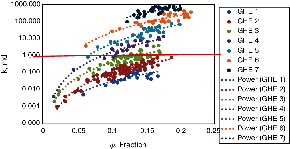
Figure 1: Rock types classification using GHE approach
Once rock types were defined, it was now possible to produce reservoir zonation based on flow units and SMLP. As it can be seen from Fig. 2, different high energy zones were identified, each with a different slope as indicated by the solid line segment. However, when a barrier separates the same slope, the layer may have 1, 2, or 3 sections, such as layer 4, which consisted of H4a, H4b, H4c, and layer 6 comprised of H6a, H6b and H6c. H refers to Hailan Formation.
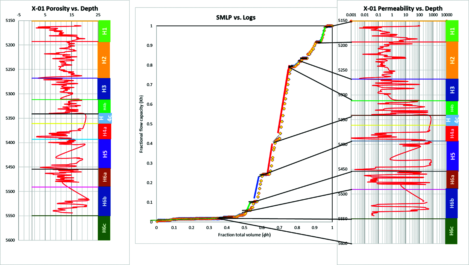
Figure 2: Reservoir zonation using SML and Logs
From SMLP there were key flow unit characteristics that can be defined as follows:
• Barriers that isolate zones as individual pressure compartment and acts as a seal.
• Baffles, which are zones block or divert the flow, commonly occur at a local scale. They might allow for minor pressure communication and limited flow.
• Speed zones: They can be fractures or vugs or high energy zones. They control primary production.
To further confirm the layering of the reservoir, Hailan formation tops were plotted with porosity and permeability, as shown in Fig. 2. From the below Figure, the quality of each layer can be seen in terms of porosity and permeability. Comparing SMLP and Logs showed that the reservoir's layering from the logs and from Lorenz plot was matched.
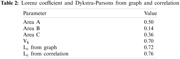
An ordered Lorenz plot was performed to indicate reservoir heterogeneity. Lorenz coefficient (Lc) can be obtained graphically or by correlation; both methods were performed to compare the results. Fig. 3 illustrates the flow capacity distribution of X-01-NX89. Graphically Lc can be obtained by calculating the area A, B and C, then dividing area C by area A.
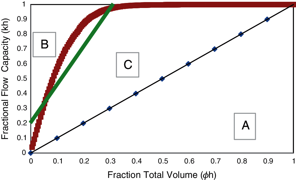
Figure 3: Ordered lorenz plot
Lc can also be obtained using Eqs. (4) and (5). From Table 2, it can be seen that the reservoir is heterogeneous. It can also be observed that both graphically and correlation methods produced similar results, which confirms that Lc values using graph and correlation were consistent and accurate.
3.4 Capillary Pressure Conversion
The Pc conversion from laboratory to reservoir condition requires values of Interfacial Tension (σ) and the contact angle (θ). Typical laboratory and reservoir values are summarized in Table 3.
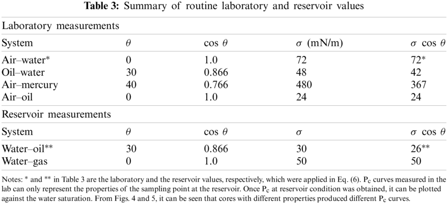
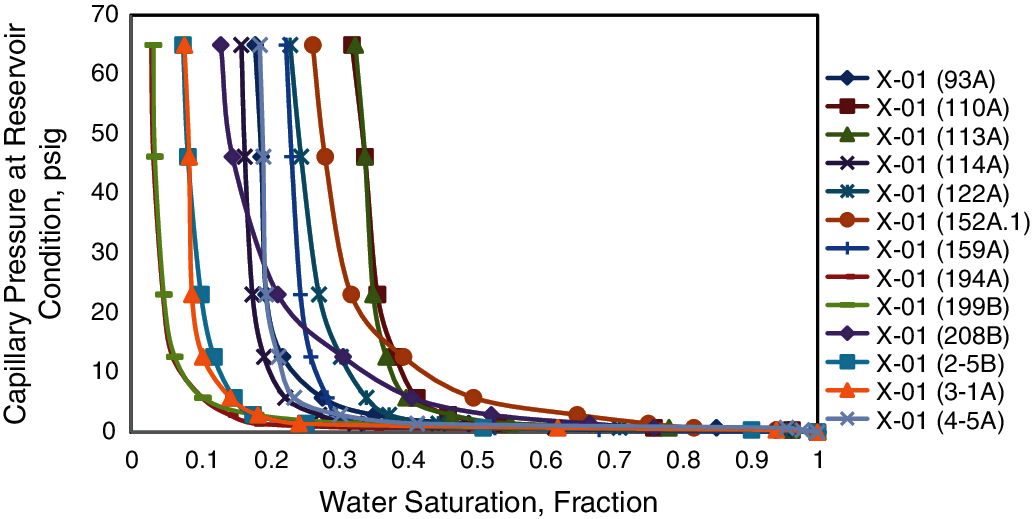
Figure 4: Pc curves at reservoir condition (scale from 0 psi–70 psi)
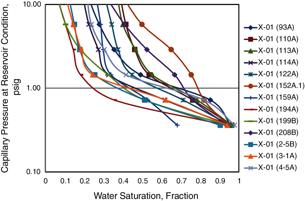
Figure 5: Pc curves at reservoir condition (scale from 0.1 psi–100 psi)
3.5 Normalized Water Saturation Calculation
Eq. (7) was used to calculate Swn for all sampled cores. The values were plotted with reservoir Pc using the multi regression method. The lithology index (J*) and the pore size distribution index (λ) were obtained. The values of (J*) and (λ) for each sample are summarized in Table 4.
According to Table 4, the steeper the slope, the lower the value of the (λ), leading to poor quality rock and less energy potential. If (λ) decreases, the rock permeability decreases, the sorting of grains is poor, and grain size might be small with lower energy profile. These will affect capillary pressure curves and shift them upwards, resulting in higher irreducible water saturation values. Before proceeding further, a regression quality check must be done to confirm the validity of the obtained data in Table 4. The value of 180 psi capillary pressure was selected, and a plot between (Sirr) and (Sw) was created. It can be seen from Fig. 6 a unit slope and a value of 1 for R2 were obtained. This implies that obtained data in Table 4 is valid and can be used to conduct further calculations such as capillary pressure or water saturation.
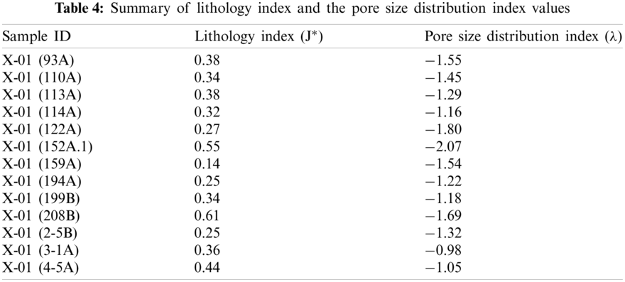
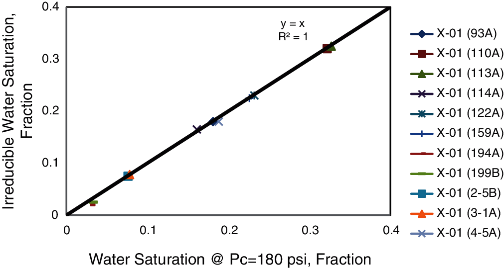
Figure 6: Data validation of lithology index (J*) and pore size distribution index (λ)
3.6 Leverett J-Function and Average Capillary Pressure Curves
Eq. (8) was used to calculate the J-function based on Pc laboratory, interfacial tension, permeability and porosity as an input. Once the calculation was done, a plot between the J-function and water saturation was obtained, as in Fig. 7. However, it should be noted that this plot was not based on the flow zone indicator technique. The scatter in Fig. 7 indicates the presence of more than one rock type and energy variation, which was investigated further in the following sections.
3.7 Classification of Average Capillary Pressure Curves Using (FZI)
Rock types were identified based on grouping similar FZI samples together, as shown in Fig. 8. According to Table 5 and Fig. 8, average capillary pressure curves can be divided into four types based on flow zone indicators.
It is now possible to plot capillary pressure curves using the J-function based on the flow zone indicator. The analysis involved averaging 13 capillary pressure curves into four main curves representing the whole reservoir, as indicated in Fig. 9. With FZI values from 3 to 9. It can be seen that with the change of the FZI value, there was a significant difference in the shape of the average Pc curves. Cores with a high FZI value showed a more extended flat segment of mercury curve, which implies a large pore throat, good sorting, and high non-wetting phase under the same pressure condition. In comparison, cores with low FZI values displayed the opposite properties: poor sorting and small pore throat.
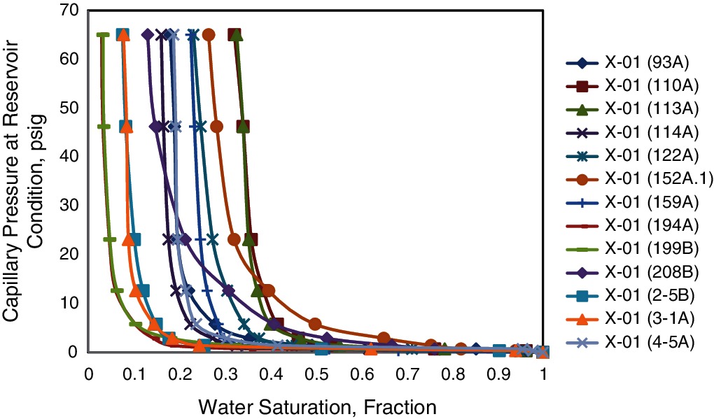
Figure 7: Capillary pressure curves using J-function
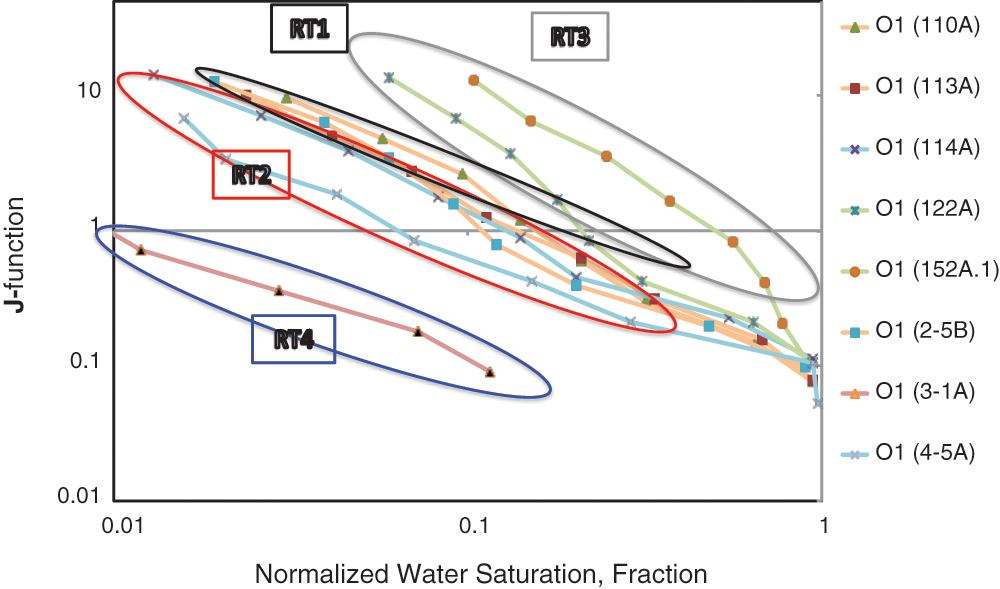
Figure 8: Rock types identification based on J-function
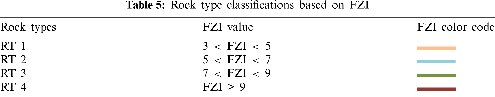
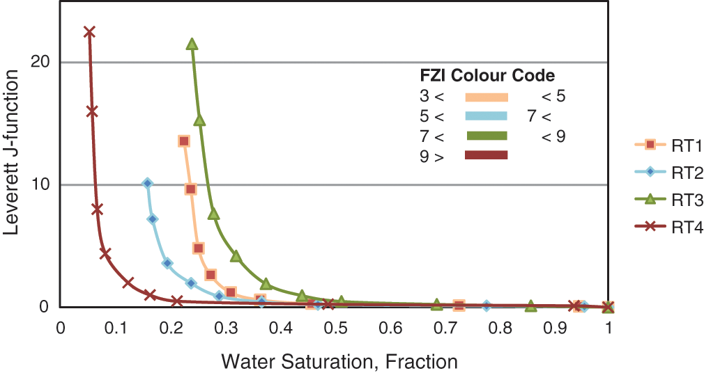
Figure 9: Capillary pressure classification based on the flow zone indicator
3.8 Capillary Pressure Calculation
Once
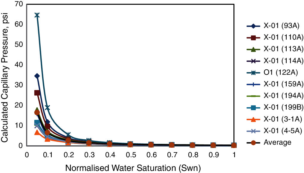
Figure 10: Capillary pressure curves
Fig. 11 illustrates a comparison between measured Pc data points and the calculated Pc line for rock type 4 (RT4). This figure shows that a good match was obtained between measured and calculated capillary pressure curves at a Pc value lower than 40 psi, which indicates that this zone is the transition zone. However, above this zone at higher Pc values, the match showed almost a similar trend. It is essential to match the log Swi for the well for successful model initialization.
3.9 Water Saturation Estimation Using J-Function
To calculate the water saturation for X-01-NX-89, the values of the coefficients a and b have to be obtained using Matlab software. A power function was first fitted to all Pc curves to find only one function as in Fig. 12 and then to all four rock types to find four functions as in Fig. 13. These functions were then used to calculate water saturation using Eq. (11), after which it was compared with the logs.
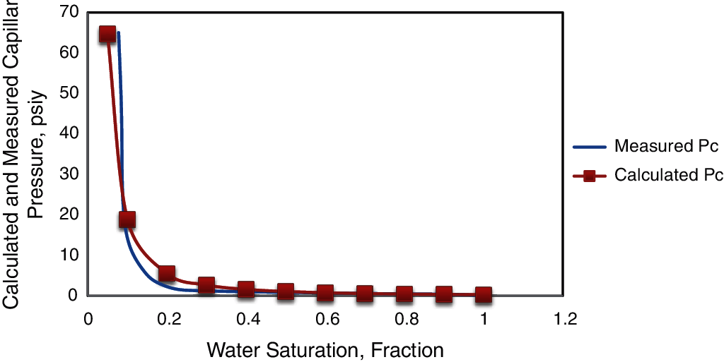
Figure 11: A comparison between measured and calculated capillary pressure for RT4
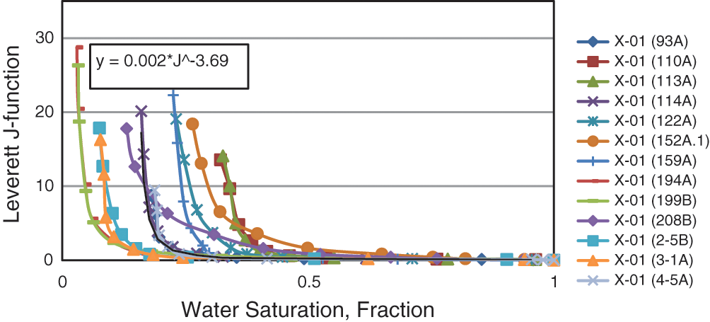
Figure 12: J-function for all Pc curves
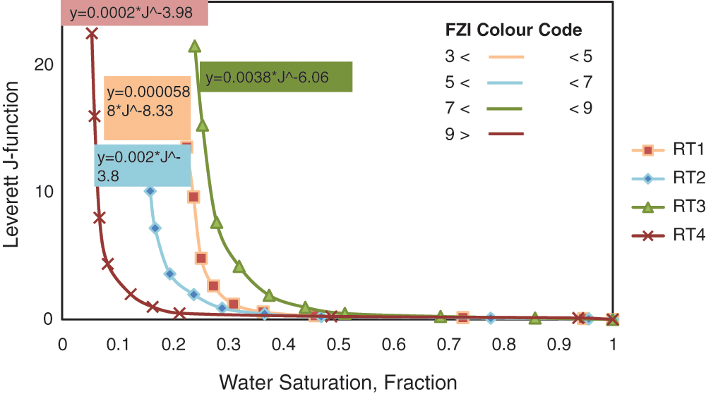
Figure 13: J-function for the four rock types
In Fig. 14, the results were fitted using one J-function, and it was found that layers (H3, H4a, H4b, and H6b) with high FZI have a smaller error in the matching process compared to layers (H4c, H5, and H6a) where there was a significant matching error. This showed that when one J-function fits the saturation, a significant error is likely to occur. FZI was different in layers where the heterogeneity of the reservoir was not taken into account. On the other hand, in Fig. 15, saturation was calculated according to rock types. A better match was observed in all the layers, especially those with high FZI. This proved that this method is effective as it improves the accuracy of the saturation calculations, leading to a better dynamic model and energy sources taking into account the heterogeneity of the reservoir.
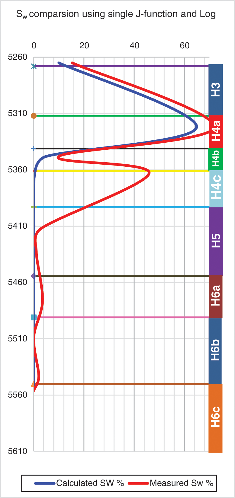
Figure 14: Water saturation using single J-function
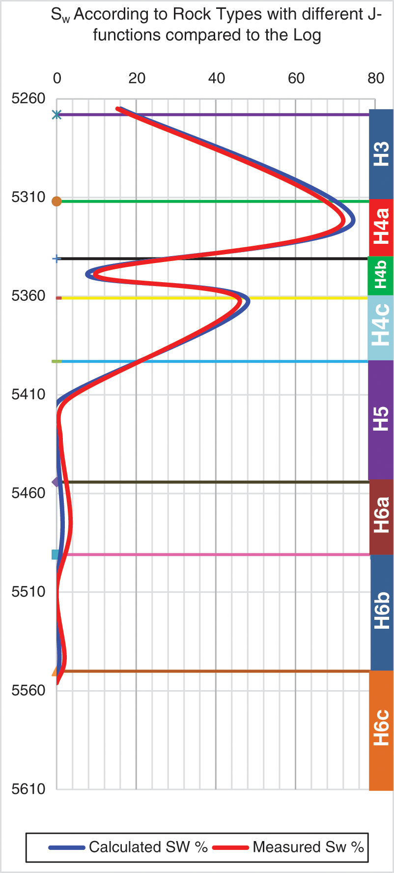
Figure 15: Water saturation using multiple J-functions
The main conclusions drawn from this study are summarized below:
• It was crucial to define advanced approaches to maximize energy sources and produce more hydrocarbon by optimizing the available subsurface energy system.
• Four Rock-types were identified by GHE using specific flow zone indicator values as a boundary between different layers to provide the reservoir description and permeability prediction. Rock types determination using this approach provided an essential understanding of factors that control the quality of the reservoir and impact the fluid flow characterization process.
• A stratigraphic modified Lorenz plot was used to conduct reservoir zonation and flow unit identification. Six layers were identified using SMLP, which confirmed the log results. Plotting core porosity and permeability on the log showed that the top layers indicated poor quality, and lower ones showed a better quality except for layers H4c and H6a. Lorenz plot showed that the total flow capacity was provided by GHE 6 and 7, whilst most of the storage is governed by GHE 4 and 5.
• Statistical analysis for the determination of reservoir heterogeneity was performed using graphical and correlational approaches. The results indicated that the reservoir was heterogeneous as the value was closer to 1. Various methods were used and compared to show that the results were consistent.
• For capillary pressure analysis, the J-function was a powerful tool to average capillary pressure curves. However, when the reservoir was heterogeneous, each sample had a different J-function shape. The more heterogeneous is the reservoir, the greater the difference in the curve shapes.
• Rock permeability and porosity play an essential role in classifying capillary pressure curves. Pc curves were averaged and classified using the J-function and flow zone indicator. Four different rock types were identified, which led to four Pc curves, with RT3 and RT4 have the best reservoir properties. This method incorporated many properties such as lithology variation, pore geometry, and water saturation.
• Pc curves were calculated, and one single Pc curve was obtained to represent the whole reservoir. A comparison between measured and calculated Pc showed an excellent match below the transition zone (40 psi), after which the match was acceptable.
• One single and multiple J-functions were used to compute the water saturation profiles for well X-01-NX-89, and the results were compared with the log interpretation. It was found that using multiple J-functions would lead to a better match between calculated and measured Sw. The result also showed that whenever the reservoir heterogeneity is strong, it is better to use the classified J-function based on FZI to calculate the water saturation. The results also indicated the higher the FZI values, the better the match will be.
Declaration of Competing Interests: The authors declare that they have no known competing financial interests or personal relationships that could have appeared to influence the work reported in this paper.
Author Contributions: All authors have contributed to writing and revising the manuscript. All authors approved the final version of the manuscript and agree to be held accountable for the content therein.
Funding Statement: The authors would like to acknowledge the financial support provided by the Universiti Teknologi Malaysia (UTM) under UTM Transdiciplinary Research Grant (Q.J130000.3551.06G68) which made this research effective and viable.
Conflicts of Interest: The authors declare that they have no conflicts of interest to report regarding the present study.
1. Mirzaei-Paiaman, A., Ostadhassan, M., Rezaee, R., Saboorian-Jooybari, H., Chen, Z. (2018). A new approach in petrophysical rock typing. Journal of Petroleum Science and Engineering, 166, 445–464. DOI 10.1016/j.petrol.2018.03.075. [Google Scholar] [CrossRef]
2. Askari, A. A., Behrouz, T. (2011). A fully integrated method for dynamic rock type characterization development in one of Iranian off-shore oil reservoir. Journal of Chemical and Petroleum Engineering, 45(2), 83–96. DOI 10.22059/JCHPE.2011.1510. [Google Scholar] [CrossRef]
3. Mirzaei-Paiaman, A., Asadolahpour, S. R., Saboorian-Jooybari, H., Chen, Z., Ostadhassan, M. (2020). A new framework for selection of representative samples for special core analysis. Petroleum Research, 5(3), 210–226. DOI 10.1016/j.ptlrs.2020.06.003. [Google Scholar] [CrossRef]
4. Mirzaei-Paiaman, A., Saboorian-Jooybari, H. (2016). A method based on spontaneous imbibition for characterization of pore structure: Application in pre-sCAL sample selection and rock typing. Journal of Natural Gas Science and Engineering, 35, 814–825. DOI 10.1016/j.jngse.2016.09.023. [Google Scholar] [CrossRef]
5. Falode, O., Manuel, E. (2014). Wettability effects on capillary pressure, relative permeability, and irredcucible saturation using porous plate. Journal of Petroleum Engineering, 2014, 465418. DOI 10.1155/2014/465418. [Google Scholar] [CrossRef]
6. Kadkhodaie-Ilkhchi, A., Kadkhodaie-Ilkhchi, R. (2018). A review of reservoir rock typing methods in carbonate reservoirs: Relation between geological, Seismic, and reservoir rock types. Iranian Journal of Oil and Gas Science and Technology, 7(4), 13–35. DOI 10.22050/ijogst.2019.136243.1461. [Google Scholar] [CrossRef]
7. Mohebian, R., Riahi, M. A., Kadkhodaie, A. (2019). Characterization of hydraulic flow units from seismic attributes and well data based on a new fuzzy procedure using ANFIS and FCM algorithms, example from an Iranian carbonate reservoir. Carbonates and Evaporites, 34(2), 349–358. DOI 10.1007/s13146-017-0393-y. [Google Scholar] [CrossRef]
8. Oliveira, G. P., Roque, W. L., Araújo, E. A., Diniz, A. A. R., Simões, T. A. et al. (2016). Competitive placement of oil perforation zones in hydraulic flow units from centrality measures. Journal of Petroleum Science and Engineering, 147, 282–291. DOI 10.1016/j.petrol.2016.06.008. [Google Scholar] [CrossRef]
9. Roque, W. L., Oliveira, G. P., Santos, M. D., Simões, T. A. (2017). Production zone placements based on maximum closeness centrality as strategy for oil recovery. Journal of Petroleum Science and Engineering, 156, 430–441. DOI 10.1016/j.petrol.2017.06.016. [Google Scholar] [CrossRef]
10. Saboorian-Jooybari, H. (2016). A structured mobility-based methodology for quantification of Net-pay cutoff in petroleum reservoirs. SPE Reservoir Evaluation & Engineering, 20(2), 317–333. DOI 10.2118/183643-pa. [Google Scholar] [CrossRef]
11. Amaefule, J. O., Altunbay, M., Tiab, D., Kersey, D. G., Keelan, D. K. (1993). Enhanced reservoir description: Using core and Log data to identify hydraulic (Flow) units and predict permeability in uncored intervals/wells. SPE Annual Technical Conference and Exhibition, Houston, Texas. DOI 10.2118/26436-ms. [Google Scholar] [CrossRef]
12. Chen, X., Yao, G. (2017). An improved model for permeability estimation in low permeable porous media based on fractal geometry and modified hagen-poiseuille flow. Fuel, 210, 748–757. DOI 10.1016/j.fuel.2017.08.101. [Google Scholar] [CrossRef]
13. Chen, X., Zhou, Y. (2017). Applications of digital core analysis and hydraulic flow units in petrophysical characterization. Advances in Geo-Energy Research, 1(1), 18–30. DOI 10.26804/ager.2017.01.02. [Google Scholar] [CrossRef]
14. Siddiqui, S., Okasha, T. M., Funk, J. J., Al-Harbi, A. M. (2006). Improvements in the selection criteria for the representative special core analysis samples. SPE Reservoir Evaluation & Engineering, 9(6), 647–653. DOI 10.2118/84302-pa. [Google Scholar] [CrossRef]
15. El Din, S. S., Dernaika, M. R., Kalam, Z. (2014). Integration of petrophysical SCAL measurements for better understanding heterogeneity effects in carbonates: Case study using samples from a super giant field in Abu Dhabi. International Petroleum Technology Conference, Doha, Qatar. DOI 10.3997/2214-4609-pdb.395.IPTC-17572-MS. [Google Scholar] [CrossRef]
16. Sharawy, E., and Nabawy, M. S., B.S. (2019). Integration of electrofacies and hydraulic flow units to delineate reservoir quality in uncored reservoirs: A case study, nubia sandstone reservoir, gulf of suez, Egypt. Natural Resources Research, 28(4), 1587–1608. DOI 10.1007/s11053-018-9447-7. [Google Scholar] [CrossRef]
17. Ahr, W. M. (2011). Geology of carbonate reservoirs: The identification, description and characterization of hydrocarbon reservoirs in carbonate rocks. New York, USA: John Wiley & Sons. [Google Scholar]
18. Shedid, S. A. (2018). A new technique for identification of flow units of shaly sandstone reservoirs. Journal of Petroleum Exploration and Production Technology, 8(2), 495–504. DOI 10.1007/s13202-017-0350-2. [Google Scholar] [CrossRef]
19. Obeida, T. A., Al-Mehairi, Y. S., Suryanarayana, K. S. (2005). Calculation of fluid saturations from Log-derived J-functions in giant complex middle-east carbonate reservoir. International Petroleum Technology Conference, Doha, Qatar. DOI 10.2523/iptc-10057-ms. [Google Scholar] [CrossRef]
20. Masalmeh, S. K., Wei, L., Hillgartner, H., Al-Mjeni, R., Blom, C. (2012). Developing high resolution static and dynamic models for waterflood history matching and EOR evaluation of a Middle Eastern carbonate reservoir. Abu Dhabi International Petroleum Conference and Exhibition, Abu Dhabi, UAE. DOI 10.2118/161485-ms. [Google Scholar] [CrossRef]
21. Khan, M. F., Al maskari, S., Kundu, A., Voleti, D. K., Al-Rawahi, A. S. (2017). Building petrophysical groups in a low permeability carbonate reservoir located in transition zone: A case study from onshore field in UAE. Abu Dhabi International Petroleum Exhibition & Conference, Abu Dhabi, UAE. DOI 10.2118/188742-ms. [Google Scholar] [CrossRef]
22. Masalmeh, S., Jing, X., Vark, W., Christiansen, S., van der weerd, H. et al. (2004). Impact of SCAL (special core analysis) on carbonate reservoirs: How capillary forces can affect field performance predictions. Petrophysics, 45(5), 403–413. DOI SPWLA-2004-v45n5a1. [Google Scholar]
23. Abedini, A., Torabi, F. (2015). Pore size determination using normalized J-function for different hydraulic flow units. Petroleum, 1(2), 106–111. DOI 10.1016/j.petlm.2015.07.004. [Google Scholar] [CrossRef]
24. El-Khatib, N. (1995). Development of a modified capillary pressure J-function. In: Middle East Oil Show, Bahrain. DOI 10.2118/29890-ms. [Google Scholar] [CrossRef]
25. Mirzaei-Paiaman, A., Ghanbarian, B. (2021). A new methodology for grouping and averaging capillary pressure curves for reservoir models. Energy Geoscience, 2(1), 52–62. DOI 10.1016/j.engeos.2020.09.001. [Google Scholar] [CrossRef]
26. Anbari, A., Lowry, E., Piri, M. (2019). Estimation of capillary pressure in unconventional reservoirs using thermodynamic analysis of pore images. Journal of Geophysical Research: Solid Earth, 124(11), 10893–10915. DOI 10.1029/2018JB016498. [Google Scholar] [CrossRef]
27. Shikhov, I., Arns, C. H. (2015). Evaluation of capillary pressure methods via digital rock simulations. Transport in Porous Media, 107(2), 623–640. DOI 10.1007/s11242-015-0459-z. [Google Scholar] [CrossRef]
28. Joshi, J. B., Nandakumar, K., Patwardhan, A. W., Nayak, A. K., Pareek, V. et al. (2019). 2-computational fluid dynamics In: Advances of computational fluid dynamics in nuclear reactor design and safety assessment, pp. 21–238. Cambridge, UK: Woodhead Publishing. DOI 10.1016/B978-0-08-102337-2.00002-X. [Google Scholar] [CrossRef]
29. Gidaspow, D. (1994). 7-inviscid multiphase flows: Bubbling beds. Multiphase flow and fluidization, pp. 129–196. San Diego: Academic Press. [Google Scholar]
30. Besnard, D. (1999). Thermal hydraulics simulations: What turbulence modeling strategies? In: Engineering turbulence modelling and experiments 4, pp. 37–48. Oxford: Elsevier Science, Ltd. [Google Scholar]
31. Elgaghah, S. A., Tiab, D., Osisanya, S. O. (2001). A New approach for obtaining J-function in clean and shaly reservoir using in situ measurements. Journal of Canadian Petroleum Technology, 40(7), PETSOC-01-07-01. DOI 10.2118/01-07-01. [Google Scholar] [CrossRef]
32. Gao, H., Yu, B., Duan, Y., Fang, Q. (2014). Fractal analysis of dimensionless capillary pressure function. International Journal of Heat and Mass Transfer, 69, 26–33. DOI 10.1016/j.ijheatmasstransfer.2013.10.006. [Google Scholar] [CrossRef]
33. Brauner, N. (2003). Liquid-Liquid Two-Phase Flow Systems. In: Modelling and experimentation in two-phase flow, pp. 221–279. Vienna: Springer Vienna. [Google Scholar]
34. Hu, Y., Yu, X., Chen, G., Li, S. (2012). Classification of the average capillary pressure function and its application in calculating fluid saturation. Petroleum Exploration and Development, 39(6), 778–784. DOI 10.1016/S1876-3804(12)60104-9. [Google Scholar] [CrossRef]
35. Westbrook, L. P., Lee, W. J. (1971). Average water saturation from capillary pressure data. SPWLA 12th Annual Logging Symposium, Texas, USA. [Google Scholar]
36. Beliveau, D. (2007). Detailed special core analysis program Key to aggressive field development planning-rajasthan, India. EUROPEC/EAGE Conference and Exhibition, London, UK. [Google Scholar]
37. Gonzalez, J. W., Perozo, A. E., Medina, F. X. (2016). Quantification of the distribution of initial water saturation through leverett J-function to calculate hydrocarbon reserves. SPE Latin America and Caribbean Heavy and Extra Heavy Oil Conference, Lima, Peru. DOI 10.2118/181177-ms. [Google Scholar] [CrossRef]
38. Deng, Y., Guo, R., Tian, Z., Zhao, L., Hu, D. et al. (2020). Water saturation modeling using modified J-function constrained by rock typing method in bioclastic limestone. Oil & Gas Science and Technology-Rev. IFP Energies nouvelles, 75, 66. DOI 10.2516/ogst/2020059. [Google Scholar] [CrossRef]
39. Farshi, M., Moussavi-Harami, R., Mahboubi, A., Khanehbad, M., Golafshani, T. (2019). Reservoir rock typing using integrating geological and petrophysical properties for the asmari formation in the gachsaran oil field, Zagros basin. Journal of Petroleum Science and Engineering, 176, 161–171. DOI 10.1016/j.petrol.2018.12.068. [Google Scholar] [CrossRef]
40. de Boer, R., Didwania, A. K. (2002). Capillarity in porous bodies: Contributions of the Vienna school and recent findings. Acta Mechanica, 159(1), 173–188. DOI 10.1007/BF01171454. [Google Scholar] [CrossRef]
41. Hoang, T. G. (2017). Defining reservoir quality relationships: How important are overburden and klinkenberg corrections? Journal of Geoscience and Environment Protection, 5(2), 86. DOI 10.4236/gep.2017.52007. [Google Scholar] [CrossRef]
42. Abbaszadeh, M., Fujii, H., Fujimoto, F. (1996). Permeability prediction by hydraulic flow units-theory and applications. SPE Formation Evaluation, 11(4), 263–271. DOI 10.2118/30158-PA. [Google Scholar] [CrossRef]
43. Kolodzie, S., Jr. (1980). Analysis of pore throat size and use of the waxman-smits equation to determine ooip in spindle field, Colorado. SPE Annual Technical Conference and Exhibition, Dallas, Texas. DOI 10.2118/9382-ms. [Google Scholar] [CrossRef]
44. Pittman, E. D. (1992). Relationship of porosity and permeability to various parameters derived from mercury injection-capillary pressure curves for sandstone. AAPG Bulletin, 76(2), 191–198. [Google Scholar]
45. Al-Qenae, K. J., Al-Thaqafi, S. H. (2015). New approach for the classification of rock typing using a new technique for iso-pore throat lines in Winland's plot. SPE Annual Caspian Technical Conference & Exhibition, Baku, Azerbaijan. DOI 10.2118/177327-ms. [Google Scholar] [CrossRef]
46. Lucia, F. J. (1995). Rock-fabric/Petrophysical classification of carbonate pore space for reservoir characterization1. AAPG Bulletin, 79(9), 1275–1300. DOI 10.1306/7834d4a4-1721-11d7-8645000102c1865d. [Google Scholar] [CrossRef]
47. Dunham, R. J. (1962). Classification of carbonate rocks according to depositional textures. Classification of Carbonate Rocks–A Symposium, pp. 108–121. [Google Scholar]
48. Jennings, J. W., Jr., Lucia, F. J. (2003). Predicting permeability from well logs in carbonates with a link to geology for interwell permeability mapping. SPE Reservoir Evaluation & Engineering, 6(4), 215–225. DOI: 10.2118/84942-pa. [Google Scholar] [CrossRef]
49. Corbett, P. W. M., Potter, D. K. (2004). Petrotyping: A basemap and atlas for navigating through permeability and porosity data for reservoir comparison and permeability prediction. International Symposium of the Society of Core Analysts, SCA2004-30. Abu Dhabi, UAE. [Google Scholar]
50. Gupta, I., Rai, C., Sondergeld, C., Devegowda, D. (2017). Rock typing in wolfcamp formation. SPWLA 58th Annual Logging Symposium, Oklahoma City, Oklahoma, USA. [Google Scholar]
51. Abdallah, S., Sid Ali, O., Benmalek, S. (2016). Rock type and permeability prediction using flow-zone indicator with an application to Berkine Basin (Algerian Sahara). SEG International Exposition and Annual Meeting, Dallas, Texas. [Google Scholar]
52. Izadi, M., Ghalambor, A. (2013). A New approach in permeability and hydraulic-flow-unit determination. SPE Reservoir Evaluation & Engineering, 16(3), 257–264. DOI 10.2118/151576-pa. [Google Scholar] [CrossRef]
53. Mirzaei-Paiaman, A., Saboorian-Jooybari, H., Pourafshary, P. (2015). Improved method to identify hydraulic flow units for reservoir characterization. Energy Technology, 3(7), 726–733. DOI 10.1002/ente.201500010. [Google Scholar] [CrossRef]
54. Shen, L., Chen, Z. (2007). Critical review of the impact of tortuosity on diffusion. Chemical Engineering Science, 62(14), 3748–3755. DOI 10.1016/j.ces.2007.03.041. [Google Scholar] [CrossRef]
55. Gunter, G. W., Sahar, M. Y., Viro, E. J., Negabahn, S., Watfa, M. (2020). Introducing a new advanced method to predict petrophysical rock types using multi-well flow units-using integrated core-log petrophysical data for identifying additional production opportunities. Abu Dhabi International Petroleum Exhibition & Conference, Abu Dhabi, UAE. DOI 10.2118/202721-ms. [Google Scholar] [CrossRef]
56. Chekani, M., Kharrat, R. (2009). Reservoir rock typing in a carbonate reservoir—Cooperation of core and Log data: Case study. SPE/EAGE Reservoir Characterization and Simulation Conference, Abu Dhabi, UAE. DOI 10.2118/123703-ms. [Google Scholar] [CrossRef]
57. Ghanbarian, B., Lake, L. W., Sahimi, M. (2018). Insights into rock typing: A critical study. SPE Journal, 24(1), 230–242. DOI: 10.2118/191366-pa. [Google Scholar] [CrossRef]
58. Gunter, G. W., Viro, E. J., Wolgemuth, K. (2012). Identifying value added opportunities by integrating well Log interpretation, petrophysical rock types and flow units; introducing a new multi-component stratigraphic modified lorenz method. SPWLA 53rd Annual Logging Symposium. Cartagena, Colombia. [Google Scholar]
59. Nugroho, C., Fahmy, M. F., Ray, D. S., Zekraoui, M., Qutainah, R. et al. (2019). Tight carbonate reservoir characterization and perforation optimization using magnetic resonance in horizontal well. SPE/IATMI Asia Pacific Oil & Gas Conference and Exhibition, Bali, Indonesia. DOI 10.2118/196383-ms. [Google Scholar] [CrossRef]
60. Muradov, K., Prakasa, B., Davies, D. (2018). Extension of dykstra-parsons model of stratified-reservoir waterflood to include advanced well completions. SPE Reservoir Evaluation & Engineering, 21(3), 703–718. DOI 10.2118/189977-pa. [Google Scholar] [CrossRef]
61. Ahmed, T. (2019). Chapter 4-Fundamentals of rock properties. In: Reservoir engineering handbook, pp. 167–281. Fifth Edition. Oxford, UK: Gulf Professional Publishing. DOI 10.1016/B978-0-12-813649-2.00004-9. [Google Scholar] [CrossRef]
62. Ahmed, T. (2010). Part 2-Fundamentals of rock properties. In: Working guide to reservoir rock properties and fluid flow, pp. 31–115. Gulf Professional Publishing, Boston. [Google Scholar]
63. Tiab, D., Donaldson, E. C. (2016). Chapter 3-Porosity and permeability. In: Petrophysics, pp. 67–186. Fourth Edition. Gulf Professional Publishing, Boston. [Google Scholar]
64. Tiab, D., Donaldson, E. C. (2012). Chapter 3-Porosity and permeability. In: Petrophysics, pp. 85–219. Third Edition. Gulf Professional Publishing, Boston. [Google Scholar]
65. Leverett, M. (1941). Capillary behavior in porous solids. Transactions of the AIME, 142(1), 152–169. DOI 10.2118/941152-G. [Google Scholar] [CrossRef]
66. Dessouky, S. (2003). A New method for normalization of capillary pressure curves. Oil & Gas Science and Technology–Rev. IFP, 58, 551–556. DOI 10.2516/ogst:2003038. [Google Scholar] [CrossRef]
67. Moradi, M., Moussavi-Harami, R., Mahboubi, A., Khanehbad, M., Ghabeishavi, A. (2017). Rock typing using geological and petrophysical data in the asmari reservoir, aghajari oilfield, SW Iran. Journal of Petroleum Science and Engineering, 152, 523–537. DOI 10.1016/j.petrol.2017.01.050. [Google Scholar] [CrossRef]
68. Trabelsi, A., Ekamba, B., Jameson, J., Schnacke, A., Jamieson, H. et al. (2009). Reservoir rock type classification and variation of reservoir quality in the arab formation, dukhan field, Qatar. International Petroleum Technology Conference, Doha, Qatar. DOI 10.2523/iptc-13628-ms. [Google Scholar] [CrossRef]
 | This work is licensed under a Creative Commons Attribution 4.0 International License, which permits unrestricted use, distribution, and reproduction in any medium, provided the original work is properly cited. |