Energy Engineering

DOI: 10.32604/EE.2022.017916

ARTICLE

Inferential Statistics and Machine Learning Models for Short-Term Wind Power Forecasting

Ming Zhang, Hongbo Li and Xing Deng*

School of Computer Science, Jiangsu University of Science and Technology, Zhenjiang, 212003, China
*Corresponding Author: Xing Deng. Email: xdeng@just.edu.cn
Received: 16 June 2021; Accepted: 19 August 2021

1  Introduction

Coal, petroleum and gas, among other non-renewable resources, will significantly contaminate the human living environment. Wind energy has gotten a lot of attention as a renewable, inexhaustible, and unlimited free energy source. Wind power is valuable not only because it is a renewable energy source, but also because of the megawatt scale of available wind turbines, easy operation, low maintenance costs and even government incentives [1–5]. According to estimates from wind power generating experts, around 2% of the sun's radiant energy is converted into wind energy each year, with installed capacity of up to 10 TW and predicted to increase even faster in the future [6–9]. In comparison to typical thermal power generation, wind energy as a type of green energy in renewable energy can lower power system running costs. As a result, a number of countries are promoting large-scale wind power development. However, the system's wind power quality is seriously impacted by the inherent randomness, intermittence, and volatility of wind power generation, and uncertainty is introduced to the system's optimal dispatch. As a result, accurate wind speed prediction can benefit not only the quality of energy, but also real-time power grid scheduling and wind farm grid-connected operation [10–14]. One of the most extensively used approaches for predicting wind speed is the neural network. Although a single hidden layer feed-forward network can be used as an efficient predictive model to fit any complex function, constructing a reasonable network model and parameters have used prior knowledge of operators is extremely difficult for researchers and engineers to achieve accurate and satisfactory results [15–18]. Wind speed is simply a time signal with several frequency components, and its spectrum may be divided into two parts: amplitude and phase. Wavelet transformation is a characterisation method that is commonly used to match input signals by scaling the parent wavelet's oscillating pattern type. Similarly, the data decomposition method may properly reflect the signal's time-frequency characteristics and assess the signal's characteristics in the time-frequency domain, allowing for signal analysis at different resolutions. For example, wavelet transformation can properly reflect signal characteristics, assess signal characteristics in the time domain and frequency domain based on a variety of resolutions. Wind power time series can be treated of a layered overlays of several frequency components with varying levels of volatility and periodicity. If multi-layer decomposition is used, a resolution with similar frequency characteristics to each decomposition component may be identified, and the resolution at different scales as well as a suitable analytical procedure can be raised. As a result, the high-precision model is developed based on the properties of each frequency component. Precision wind energy forecasting can combine many volatile power sources at all levels of the transmission and distribution networks [19–24]. Short-term wind power forecasting with high accuracy might be considered an effective method for reducing grid integration and energy trading challenges [25–31]. The short-term wind is random, whereas the long-term wind follows a continuous probability density function, often known as the “Weibull distribution.” Physical models and statistical methods are the mainly two kinds of short-term forecasting methodologies. The former method necessitates a great deal of physical data about the wind turbine, but the later usually treated as a soft computing method, is more adaptable and simple to apply in practice.

The accuracy of wind speed and wind power predictions is usually influenced by the surface wind, precipitation probability, maximum temperature, and even the conditional probability of frozen precipitation. In short-term wind power forecasting, wind speed is the most important meteorological component. Stetco et al. [32] provided a bibliographical assessment of general trends in the realms of wind speed and wind power forecasting. For the wind speed forecasts, numerical wind speed predictions based on Kalman filtering [33] and atmospheric models [34] with varied horizontal resolution capabilities were applied. Neural networks in combination with nearest neighbor search methods [35] were used to predict the output power of a specific wind farm using evolutionary optimization algorithms. The current state of hybrid solar-wind power generation system simulation, control, and optimization is described in [36,37]. The sensitivity of conventional generation and transmission were investigated as an example of alternative methodology using a static linear programming model. Deng et al. [36] developed a model for analyzing system optimum configurations based on the probability of power supply loss in hybrid solar-wind systems (LPSP). Deng et al. [38] investigates the uncertainty of wind power forecasting (WPF) using a proposed stochastic model. Tayab et al. [39] proposed some strategies for forecasting grid loads, with two main topics being discussed: short-term load forecasting (STLF) and the influence of anthropologic and structural variables on forecasting accuracy. The following issues are what we want to address in this paper based on the above discussion:

The methods to select the variables among the many available meteorological variables which has a substantial impact on the output power prediction accuracy, should be considered.

The short-term wind power forecasting category and error distribution in benchmark models.

This paper is organized as follows: data description and preprocessing, correlation analysis and neural network-related approaches are provided in Section 2. Section 3 introduces short-term wind power forecasting results obtained by the benchmark approaches, such as persistence, LMNN, NARX network, RNN and LSTM network, and all the performance of employed approaches via an illustrative example are also demonstrated. In Section 4, proposed results and prospective research issues are summarized and discussed.

2  Proposed Approaches for Wind Power Forecasting

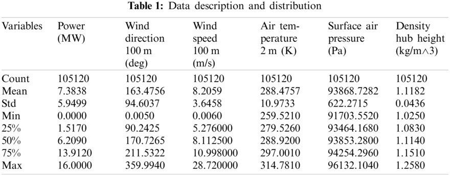
The basic data description and distribution, data preprocessing methods, forecasting categories, and forecasting form are presented first in Fig. 1 of the paper's processing diagram. Second, correlation analysis between variables is used to select the input variables for describing output power with the fewest input variables. Furthermore, a heatmap of the correlation matrix between all of the available variables in Table 1 is shown, and a summary of the data distribution is provided by wind rise related to wind speed. Finally, five neural network-related benchmark approaches, such as the persistence model, LMNN, NARX network, LMRNN, and LSTM network, are shown to illustrate the short-term wind power forecasting accuracy.

2.1 Data Description and Preprocessing

The dataset is provided by the Software Engineer Divyam Khandelwal [40] and download from the Github, which is a time series with Power (MW), Wind direction 100 m (deg), Wind speed 100 m (m/s), Air temperature 2 m (K), Surface air pressure (Pa) and Density hub height (kg/m∧3), for the time period from 2012.01.01 to 2012.12.31. The detailed information of the considered dataset is given in Table 1.

The values of ‘Hour’ ranges from 0 to 23, which indicates the number of hours-ahead needed to be forecasted in short-term. For convenience, all the dataset objects are converted in to the standardized ISO 8601 format by following the processing procedure proposed by data scientist Jon Lo. Correspondingly, the forecasting category is split into two following categories:

Category 1: 1 h to 12 h ahead data

Category 2: 13 h to 24 h ahead data

Assume variables listed in Table 1, such as wind power yt(pow), wind speed xt(win) and wind direction xt(dir)etc. at t-th time, then the forecasting is organized by

yt+k(pow)=.[yt(pow),…,yt−my(pow),…,xt(win),…,xt−mx(win),xt(dir),…,xt−mu(dir),…](1)

where py and px are positive integrate, indicating the model lags associated to wind power yt(pow) and wind speed xt(win) at t-th time, respectively. yt+k(pow) and (yt(pow),…,yt−py(pow),…,xt(win),…,xt−px(win)) are the outputs and inputs, respectively. k∈N+ is a factor to measure the k-ahead forecasting interval used to represent the short-term, median-term or long-term forecasting.

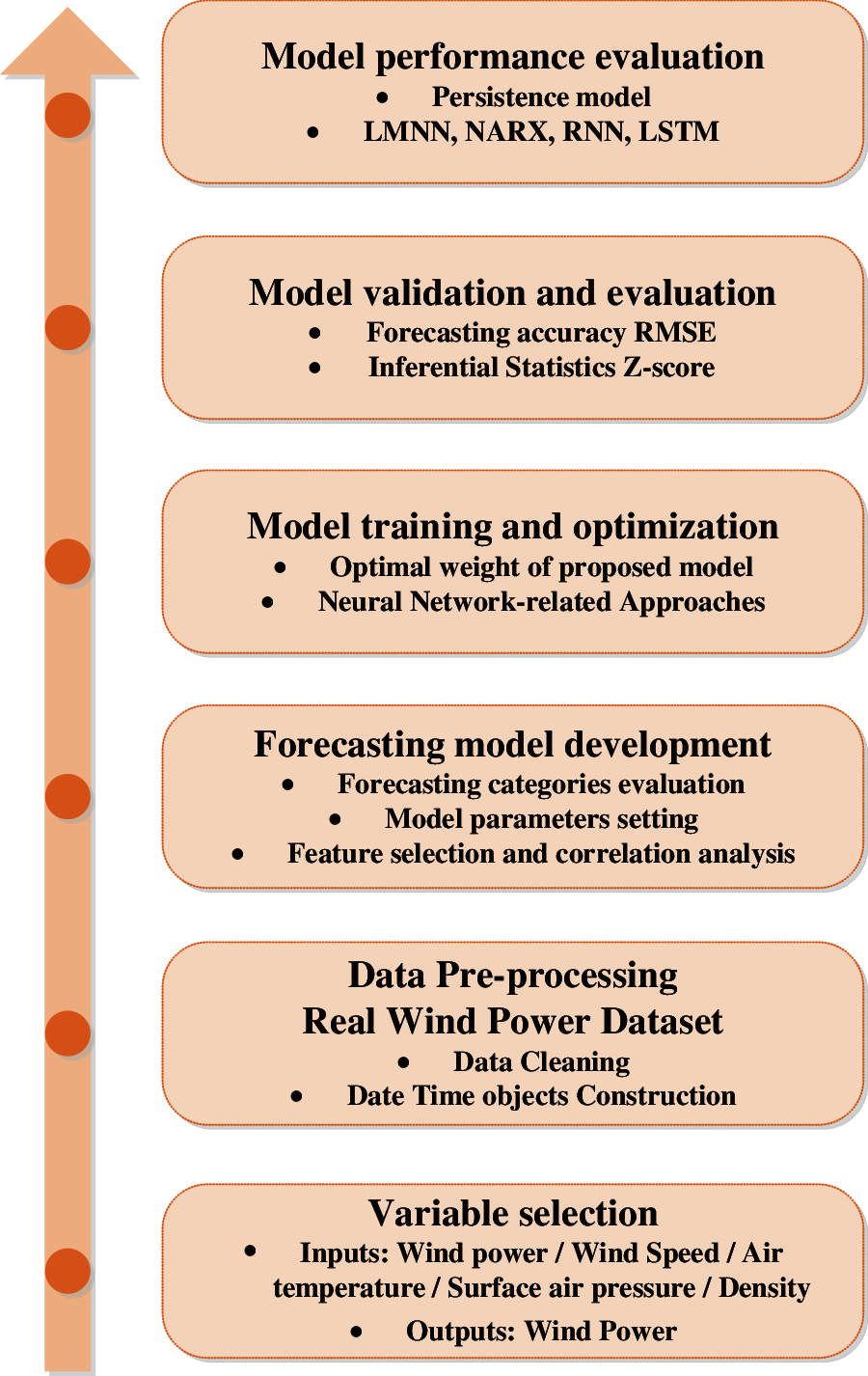
Figure 1: The processing diagram of this paper

2.2 The Correlation Analysis between Variables

An ideal variable input is one that is extremely informative, especially when it is independent of each other, has a good number, and can be utilized to generate a set of variable interpretations. As a result, the ideal input variables will have the fewest input variables to represent the characteristics of the output variables, which promotes neural network structural design and promotional capacities. For linear argument selection approaches, there are forward-back and step-by-step regression methods. In reality, selecting procedures for nonlinear arguments remains a major challenge. Researchers are gradually learning various climate characteristics of wind power, as well as the feedback impact of wind power, radiation, and precipitation, mainly to the use of ground observation data. Station observation, on the other hand, has its own intractable flaws, such as wind power overlap error, weather dependence, and observation area constraints.

cov(Xi,Xj)=∑k=1,…,m(xki−x¯⋅i)(xkj−x¯⋅j)m−1(2)

where X=[X1,X2,⋯,Xn]T,{xk⋅=[xk1,xk2,⋯,xkn]T|1≤k≤m}, Xi and Xj represent two arbitrary variables selected from the Table 1, x¯⋅i and x¯⋅j are the expectation value of the time series xk⋅, and m is the length of the given wind power data. Correlation coefficient cov(Xi,Xj) is used to reflect the degree of correlation between different variables. The product difference approach is used to determine the correlation coefficient, which represents the degree of correlation between different wind power variables and their respective mean values. Because the mathematical expectation of the variable cannot be determined, the m−1 reflects the sample mean of the random variable.

2.3 Neural Network-Related Approaches for Forecasting

The robustness of the artificial neural network can be determined by the network parameters and the specific morphology of the error surface around the sample (ANN). The network parameters can be coupled to the sample extreme points to make the network more resilient, and the resulting error surface distribution is generally flat. It is critical to evaluate the network output's resilience, which may help address practical difficulties and improve the network's promotion ability and application prospects. The input is effectively a set of feature vectors composed of the available variables from Table 1, and a typical neural network input-output mapping is given by

f(x)=∑j=1mwjφ(||x−xj||)(3)

where m, wj and φ(||x−xj||) are the number of hidden nodes in hidden-layers, the adjustment weight and a set of m arbitrary functions, respectively. In order to speed up convergence, the weights of the output layer are frequently modified quickly using a linear optimization technique, while the activation functions of the hidden layer are processed slowly using nonlinear optimization strategies. An isotropic Gaussian mapping defined by

δ=dmax2P(4)

with standard deviation is typically used according to the spread of the centers, where dmax is the maximum distance between the chosen centers. The least mean square approach used for the weight adjustment defined by

ΔWk=η(dk−WkTΦ)Φ(5)

are applied to the weights of output layers, where Wk and dk are the corresponding linear weight and the desired output, respectively. If a high-accuracy forecasting model is used, the time-delay must be taken into consideration while estimating wind power in the short future. NARX (Nonlinear autoregressive with external input) helps improve historical data memory and is an important component of a dynamic neural network. The NARX network's training function is a Bayesian regularization based on Levenberg-Marquardt optimization that updates the network's weight and bias values and minimizes a linear combination of squared errors and weights to ensure that it is properly generalized. Typical performance functions are usually measured in practice by

MSE=1N∑i=1,…,Nei2,ei=ti−yi,i=1,…,N(6)

MSW=1N∑i=1,…,Nωj2(7)

MSEreg=γMSE+(1−γ)MSW(8)

where γ is the performance ratio. MSE and MSW are the mean sum of squares of network error and biases, respectively.

2.4 Performance Evaluation Metrics

The mean square error (RMSE) is used to predict the degree of discreteness or deviation between the desired output and forecasted ones, to measure the accuracy of the prediction, defined by

RMSE=1n∑t=1,…,n(ytf−y^tr)2(9)

The new performance function RMSE leads the network to have smaller weights and biases, resulting in a smoother network response and less overfitting of the equation. In its most primitive sense, an RBF neural network has three layers with only one hidden layer that executes a nonlinear transition from input space to hidden space. It has a higher learning efficiency and function approximation than the BP network.

Experiments

3.1 Analysis of the Forecasting Categories and Data Distribution

The pd.DataFrame.merge are applied to mearge the training sample with wind speed and wind power, and the mean wind speed, wind power and wind direction is 8.1951, 163.3769 and 0.461702, respectively. The curve of wind speed data for the whole year from January 2012 to December 2012 is shown in Fig. 2, and two forecasting categories with respect to wind speed are visualized in Fig. 3.

The distribution pattern of wind speed under different forecasting categories is generally different, regardless of whether longer or shorter forecasting is used, and the inferential statistics results in Section 3.3 can still confirm the highlighted issue. The wind rise in relation to wind speed is shown in Fig. 4, which suggests a concise view that wind speed and direction are commonly dispersed at 0∼15 m/s (about 60%–70%). The wind speed has been concentrated in three directions: 135–180 degrees, 225–260 degrees, and 270–350 degrees. The geological or meteorological aspects may be to blame for these discrepancies in data distributions.

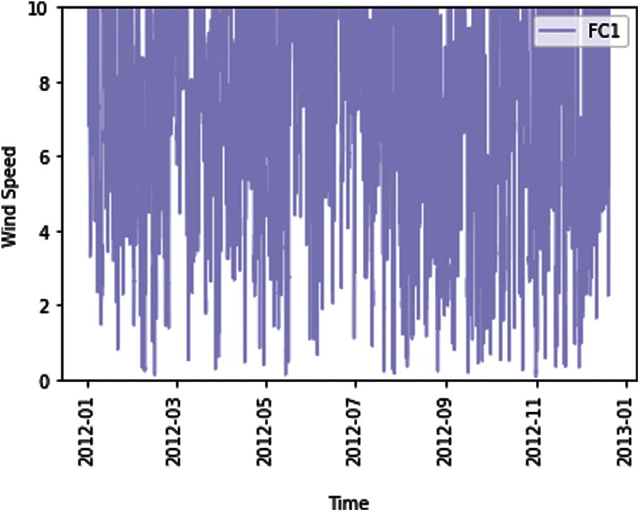
Figure 2: The wind speed trajectory of the whole year in 2012

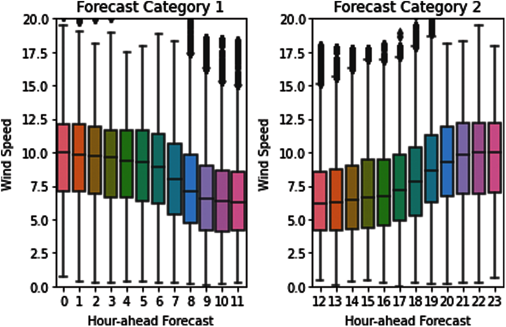
Figure 3: Two forecasting categories

3.2 Correlation Analysis between Variables

Figs. 5–6 show the correlation analysis and the accompanying heatmap of correlation matrix of the available variables in Table 1. To illustrate correlation estimation between distinct variables, we introduced Pearson correlation coefficients in Fig. 5. It is simple to see that there's a significant correlation between wind speed and output power, with a coefficient of 0.96, fitting the high correlation's range of 0.9–1.0, notably the (a) and (b) of Fig. 6, which show that the coefficient of wind power and wind speed are the highest. Because their correlation coefficients (about 0.0051) are the lowest, there is a weak link between wind power and density hub height (kg/m3), which is followed by wind direction and air temperature 2 m (K) (correlation coefficients is about 0.0092 and 0.0051, respectively). This is particularly evidence that the randomness, intermittence, and seasonality of natural wind speed, as well as the wind power of wind turbines proportional to wind turbines, and the output voltage of wind turbines, are all closely related to wind speed fluctuations. Wind speed, to be more specific, has a considerable impact on wind power forecasting accuracy.

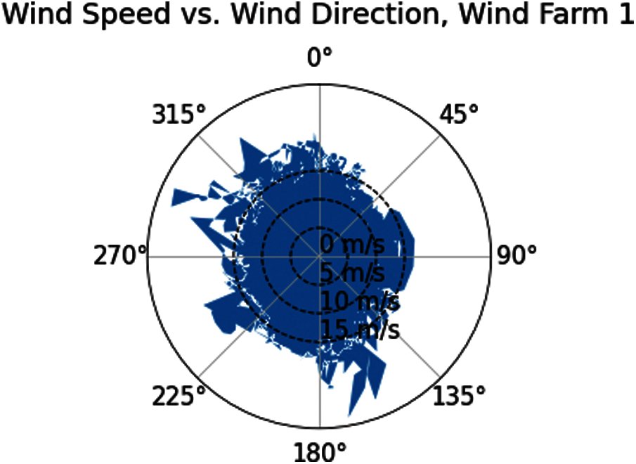
Figure 4: Wind rose of wind speed

3.3 Inferential Statistics and Performance Evaluation

Inferred statistics are statistical methods for inferring population characteristics from selected samples. It have been used to compare forecasting categories to see if there are differences between them: Forecast Category 1 (0–11 h ahead) and Forecast Category 2 (12–23 h ahead). Assume the μ1 and μ2 are respectively, the mean of two outlined forecasting categories, the null hypothesis is

and the z-tests for the null hypotheses is setting as Z = 1.96 and significance level α = 0.05, based on the evluation results, Z-test statistic formular is defined as Z=m−μs⋅n.

Z scores is 36.6413 which is greater than z-tests scores Z = 1.96. This indicates that the two forecasting models are significantly different. In addition, as the number of forecasting steps increases, the accuracy of the forecasting will decrease dramatically. In short-term wind power forecasting, a tiny error can nonetheless result in large forecasting inaccuracies. This also shows that there is a distinction between two types of short-term wind power predictions. Table 2 shows the short-term wind power forecasting results based on benchmark methodologies. In Table 2, LMNN: Multilayer Perceptron with LM learning methods; NARX: Nonlinear autoregressive exogenous neural network model; LMRNN: RNNs with LM training methods; LSTM: Long short-term memory neural network.

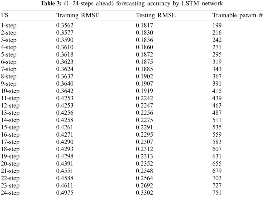
Forecasting results 1–24-steps ahead wind power forecasting is obtained by LSTM network and tabulated in Table 3. The forecasting results denote that the forecasting performance deteriorates and the forecasting accuracy decreases with the increase in forecasting-steps. The slight inaccuracy in wind speed forecasting usually translates to large errors in wind power predictions. This means that, in addition to the proposed approach in this research, the forecasting model should be capable of error correction, dynamical feedback, and adaptive adjustment.

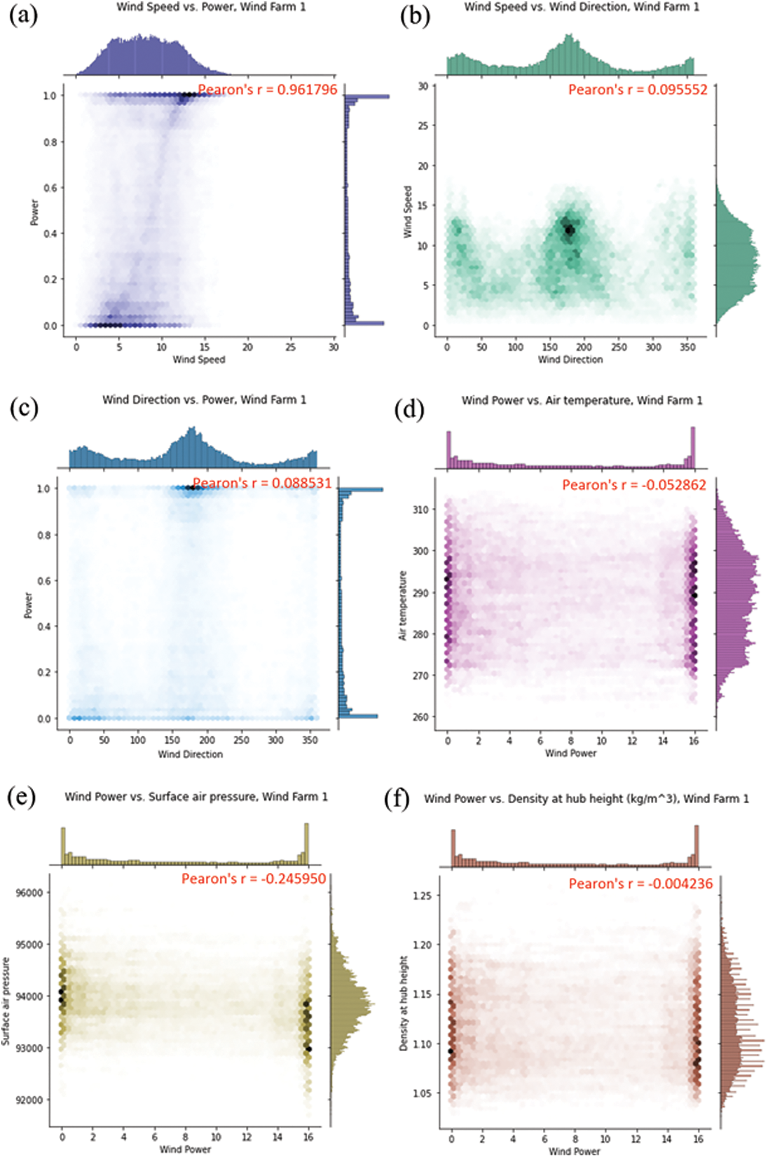
Figure 5: Visualization of correlation analysis (a) Wind speed vs. wind power; (b) Wind speed vs. wind direction; (c) Wind direction vs. wind power; (d) Wind power vs. air temperature; (e) Wind power vs. surface air pressure; (f) Wind power vs. hub height

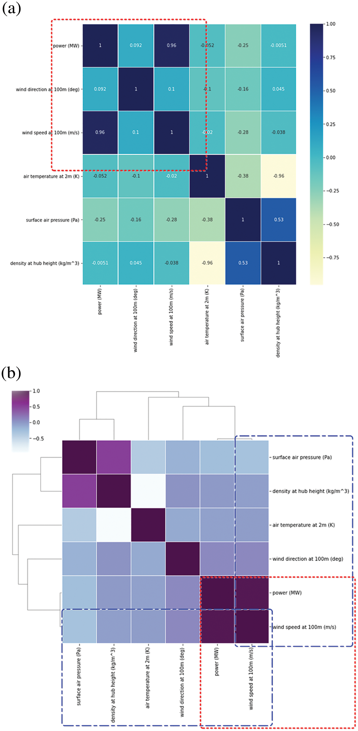
Figure 6: Heatmap of correlation matrix (a) Heatmap of correlation matrix; (b) Heat map derived from correlation matrix

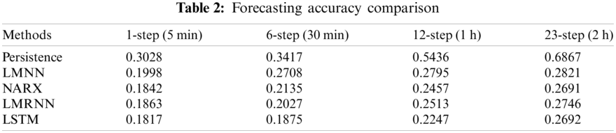
Training, validation and testing samples of the wind power and wind speed are shown in Fig. 7, and the training and validation curve of the cost funtion (1-step to 24 steps ahead forecasting) is provided in Fig. 8. There is a considerable difference between the two forecasting groups, as discussed previously. Because the persistence model assumes that the present data and the predictor do not change, and infers the predicted value based on inferential analysis, taking into account the 23-steps ahead forecasting outcomes, its forecasting accuracy is considerably lowered with RMSE 0.6867. When compared to the findings obtained by the other five forecasting models, this model has the lowest forecasting accuracy. The LSTM and NARX models share the best predicting results overall with the other approaches because they incorporate the delay and feedback mechanisms of wind power time series and boost the recall ability of historical data. One of the most generally used models of circulatory neural networks is the long-term short-term memory (Long Short-Term Memory, LSTM) network. This addresses two major flaws in simple circulatory neural networks: exploding gradients (i.e., it is trivial to generate infinite and non-values, resulting in data overflow owing to the bigger gradient value) and vanishing gradients (i.e., the learning ability of the model decays and the quality of learning is reduced when gradient values are small or even tend to zero). As a result, the five benchmark techniques have the best predicting accuracy, which is 62.43%, 8.54%, 4.12% and 6.05% lower than the other four models.

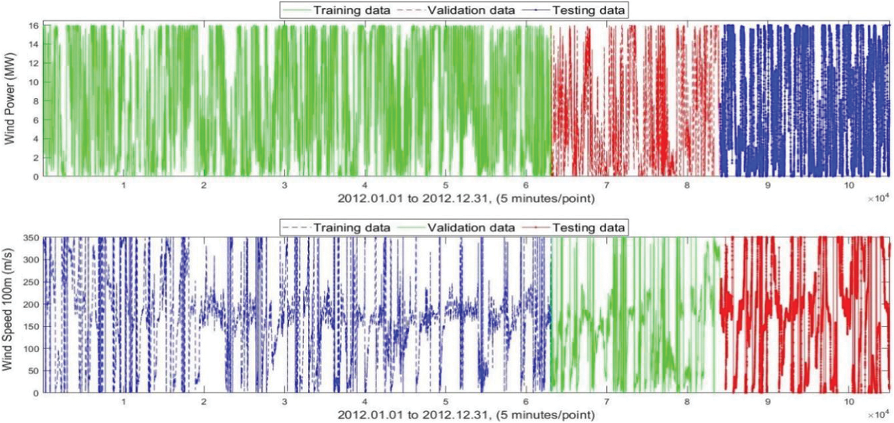
Figure 7: Training, validation and testing samples of the wind power and wind speed

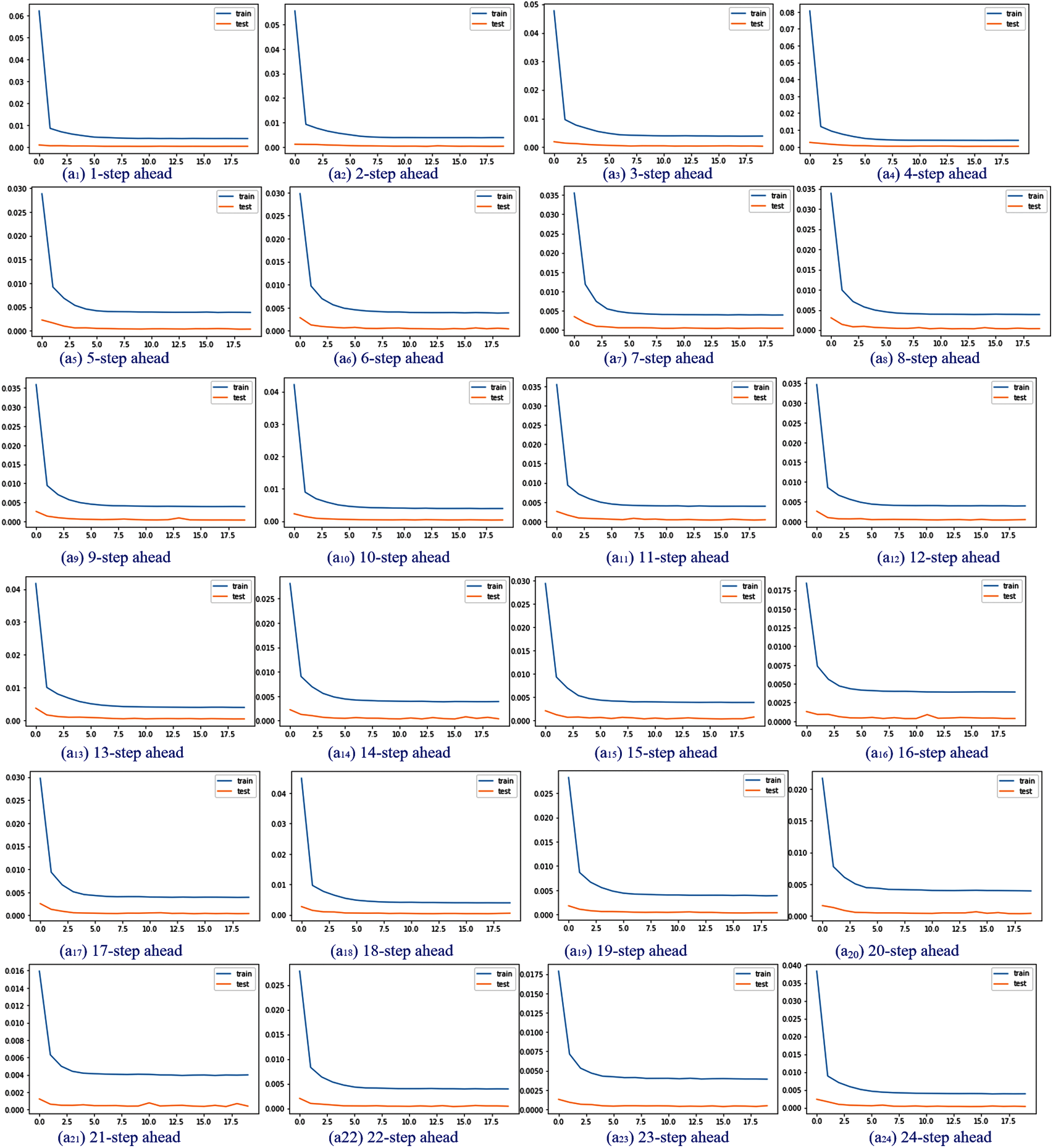
Figure 8: The training and validation curve of the cost function (1-step to 24 steps ahead forecasting)

4  Conclusion

Inferred statistics are used in this research to confirm that there is a significant difference between the two forecasting groups, i.e., Forecast Category 1 (0–11 h ahead) and Forecast Category 2 (12–23 h ahead) are the two types of forecasts. The wind speed has a significant impact on the forecasting accuracy of wind power when compared to the wind direction, air temperature 2 m (K), surface air pressure (Pa), and density hub height (kg/m3) based on the correlation analysis. To verify the final performance of the forecasting output, five benchmark methodologies are used: persistence model, LMNN, NARX network, LMRNN, and LSTM. For accurate and dependable wind power forecasting, we would use dynamical analysis with error correction capability in combination with reinforcement learning in the future.

Acknowledgement: The authors acknowledge the reviewers providing valuable comments and helpful suggestions to improve the manuscript.

Funding Statement: This research is supported by National Natural Science Foundation of China (No. 61902158).

Conflicts of Interest: The authors declare that they have no conflicts of interest to report regarding the present study.

This work is licensed under a Creative Commons Attribution 4.0 International License, which permits unrestricted use, distribution, and reproduction in any medium, provided the original work is properly cited.