| Energy Engineering |
DOI: 10.32604/ee.2022.016657
ARTICLE
A Value-at-Risk Based Approach for PMU Placement in Distribution Systems
College of Electrical Engineering, Guizhou University, Guiyang, 550025, China
*Corresponding Author: Min Liu. Email: ee.mliu@gzu.edu.cn
Received: 13 April 2021; Accepted: 23 August 2021
Abstract: With the application of phasor measurement units (PMU) in the distribution system, it is expected that the performance of the distribution system state estimation can be improved obviously with the PMU measurements into consideration. How to appropriately place the PMUs in the distribution is therefore become an important issue due to the economical consideration. According to the concept of efficient frontier, a value-at-risk based approach is proposed to make optimal placement of PMU taking account of the uncertainty of measure errors, statistical characteristics of the pseudo measurements, and reliability of the measurement instrument. The reasonability and feasibility of the proposed model is illustrated with 12-node system and IEEE-33 node system. Simulation results indicated that uncertainties of measurement error and instrument fault result in more PMU to be installed, and measurement uncertainty is the main affect factor unless the fault rate of PMU is quite high.
Keywords: Distribution system state estimation (DSSE); efficient frontier; meter placement; phasor measurement units (PMU); value at risk (VaR); weighted least square (WLS)
State estimation (SE) is a function that takes advantage of the inherent redundancy among the available measurements in order to determine the best estimate of the system states defined as the set of all the bus voltage magnitudes and phase angles in the system [1]. In the distribution system, it is not economically feasible to install a lot of measure devices to monitor, protect and control the distribution system. SE is the basic function of the Distribution Management System (DMS) of the distribution grid, which provides the required state values to the advanced DMS functions such as distribution contingency analysis, optimal network reconfiguration, fault location and restoration, demand response, voltage and var control, and var optimization et al. Recently, with the development of the application of phasor measurement units (PMU) in the distribution system [2–4], synchronized phasor measurements are introduced into the SE process. It was demonstrated that the estimation accuracy of the SE can be improved obviously with the PMU measurements into consideration (e.g., in [5–7]). Since it is not possible to install the PMUs at every node in the distribution system due to the economic consideration, we have to make a tradeoff between improving SE performance and saving cost by appropriately allocating PMUs among the distribution system, which is an optimal problem of measurement placement. Furthermore, it is worth to consider that a PMU, as a kind of measure instrument, has measure error and may faults during operation, i.e., when we solve the optimal placement problem we should consider the uncertainty of measure errors and the reliability of the measure instruments.
For the SE performance, traditionally, there are three evaluation metrics: estimation accuracy, observability of the system, and numerical stability of the estimator. In the literature of SE in the transmission system, the objective of the meter placement is mainly to improve the network observability (e.g., [8–13]) or minimize the estimation errors, i.e., maximize estimation accuracy (e.g., [14,15]). As for the SE in the distribution system level, there are not enough real measurements in the distribution system and pseudo measurements are introduced to solve the observability problem in practice. Due to the large number of pseudo measurements, compared with the improvement of estimation accuracy, the improvement of system observability by PMU installation is limited. Therefore, estimation accuracy is adopted to evaluate the SE performance in the distribution system by a vast majority of research literature on PMU allocation [16–19]. As to how to quantify the estimation accuracy, there are mainly three types of accuracy indices: variance of estimates [20], estimate errors in voltage magnitude and angle [5,21–24], variance of estimate errors [1,25–27]. Variance of estimates or variance of estimate errors describe the uncertainties of the SE results but do not give an intuitive description on the estimation accuracy. It is, therefore, not appropriate to use the variance as the accuracy index when decision makers make a tradeoff between accuracy and cost. Estimate errors give the estimation accuracy intuitively, but do not give the information about the uncertainties in the SE process, e.g., the uncertainties of measurement errors and instrument fault.
With regard to the tradeoff between the estimation accuracy and cost, few papers address this problem. Pegoraro et al. [24,25] solved it as a weighted multi-objective problem in which how to decide the weights of accuracy and cost is an issue and need further research.
As for the uncertainty of measure errors, most of the papers adopt Monte Carlo simulation based on a given probability distribution of the measure errors. For the reliability of the measure instruments, Liu et al. [25] addressed it with traditional N-1 criteria. But N-1 is a subjective judgment and does not consider the probability of the instrument failure.
Addressing the above problems, i.e., i) How to quantify the estimation accuracy with an intuitive index taking account of the uncertainties in the process of SE? ii) How to make a tradeoff between the accuracy and cost? iii) How to address the reliability problem of the measure instruments), this paper proposed a framework for the optimal allocation of PMU in the SE of the distribution system based on the concept of efficient frontier and value at risk (VaR), and developed a Genetic Algorithm (GA) based approach to solve the proposed optimization model since GA is a widely used optimization algorithm and has been used in the optimization of PMU configuration [23,28,29].
The main innovations of this paper are as follows: i) VaR index is used to quantify the impact of uncertain factors such as PMU fault and measurement error on the accuracy of state estimation (compared with the Variance index used in most literatures, VaR can give an intuitive description of the uncertainty of estimation accuracy, which is helpful for decision makers to make a choice between Cost and Accuracy), ii) Based on the concept of Pareto optimality, a VaR-Cost effective frontier decision model is established to facilitate decision makers to select the Optimal PMU configuration scheme according to their own investment scale or estimation accuracy requirements (this scheme has fully considered PMU failure, measurement error and other uncertain factors).
In the following, Section 2 first introduces the decision criteria, uncertainties to be considered, the decision framework and the corresponding mathematical model; then Section 3 describes how to solve the proposed optimization model based on the GA approach; after then Section 4 gives the simulation based a 12-node system and the corresponding analyses; finally Section 5 summarizes the paper and discusses the future work.
As discussed above, an optimal PMU allocation (i.e., the optimal PMU placement) is the one which has higher estimation accuracy with lower investment cost taking account of the associated uncertainties.
In order to make a tradeoff between the accuracy and cost, we apply the concept of efficient frontier to establish the optimization model of PMU placement. Efficient frontier has been widely used in the investment literature to solve portfolio issues [30]. In the paper, the efficient frontier is defined as a frontier which consists of all PMU portfolio points which have the maximum estimation accuracy for a given invest cost (Fig. 1). A PMU portfolio is a combination of quantities and locations of PMUs which describes how many PMUs are installed and where to install them. Based on the formed efficient frontier, decision-makers can choose the optimal PMU portfolio according to their accuracy expectation and/or cost limitation.
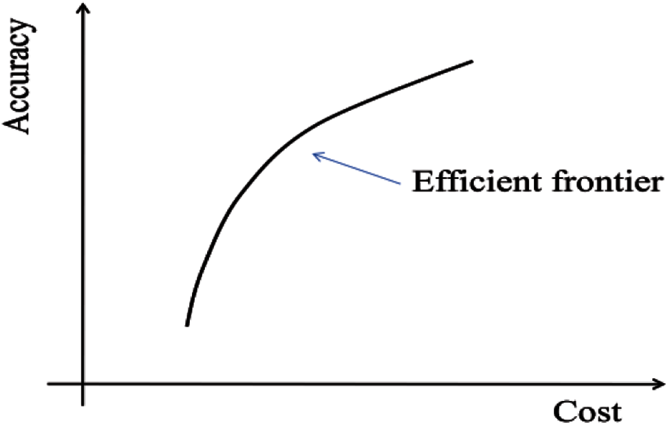
Figure 1: Efficient frontier
In the process of forming the efficient frontier, the associated uncertainties, such as the uncertainty of measure errors and instrument failures, are modeled based on the Monte Carlo simulation approach. In the following, we introduce the uncertainties considered, the accuracy index taking into account of uncertainties, and the mathematical model of the PMU placement.
There are three types of uncertainties considered in the paper, i.e., i) random fluctuation of loads, ii) measure errors of the measurement instruments, and iii) possible fault occurring in measurement devices.
For those load nodes without real measurements, pseudo measurements are adopted in the SE of distribution system in order to meet the observability requirement. Since pseudo measurements are obtained through modeling or forecasting loads based on historical data and in the reality loads fluctuate randomly, pseudo measurements are therefore random variables. In the paper, we suppose pseudo measurements are normally distributed or uniformly distributed and analyze their affect on the optimal PMU allocation in Section 4. Here, loads refer to general loads which include both customers consuming electricity and distributed generators producing electricity.
For those nodes with real measurements, their measure values are also random variables since there exists measure errors arising from i) inaccurate transducer calibration, ii) the effect of analogue-to-digital conversion, iii) noise in communication channels, and iv) unbalanced phases, etc. [31]. In the SE literature, measure errors of the real measurements are supposed normally distributed.
For the real measure devices, except for the uncertainty of measure errors, they have the uncertainty of device failure in the operation. In the paper, we suppose the fault probability of the measure device is known based on the operation data, and adopt Monte Carlo simulation to model the randomness of the device fault.
In order to judge the estimation error intuitively, in the paper, estimation error is expressed as the relative error in percentage. Therefore, estimation accuracy rate (Acc) is defined as:
where
In the paper, the accuracy index,
There are numerous methods to calculate VaR, Jorion et al. [32] distinguishes four separate routes to measuring VaR: delta-normal method, historical simulation, stress testing method and Monte Carlo approach. This paper adopts the Monte Carlo approach, i.e., based on N times simulations, sorting the estimation accurate rate in descending order, and the value of
Based on the above definition of the accuracy index, the efficient frontier can be formed by maximizing accuracy index,
where
where
z is the set of measurements, x is the vector of the state variables which refer to voltage angle and voltage magnitude in the paper, e is the measurement error vector,
In the SE, traditional measurements include voltage magnitude
where
p=a, b, c for three phases,
where
For the solution of problem (4) the conventional iterative method is adapted by solving the following normal equation at each iteration k to compute the correction
where
is the gain matrix, H is the Jacobian of the measurement function
This paper applies genetic algorithms (GA) to solving the above optimization problem (2). As summarized by [35], the genetic algorithm maintains a population of individuals for each generation. Each individual represents a potential solution to the problem at hand. Each individual is evaluated to give some measure of its fitness. Some individuals undergo stochastic transformations by means of genetic operations to form new individuals. There are two types of transformation: mutation, which creates new individuals by making changes in a single individual, and crossover, which creates new individuals by combining parts from two individuals. New individuals, called offspring, are then evaluated. A new population is formed by selecting the more fit individuals from the parent population and the offspring population. After several generations, the algorithm converges to the best individual, which hopefully represents an optimal or suboptimal solution to the problem.
In this paper, an individual is a vector, y, which has the same number as that of the potential installation node of PMU and its components are simply binary values (0/1), corresponding to the installation status of PMU (without/with) at a given node. That is, an individual is a PMU portfolio (PMU placement combination). The detailed optimization procedure is shown in Fig. 2. i.e.,
Step 1: let the cost equal to the minimal cost, i.e., the cost of installing one PMU;
Step 2: find the optimal PMU portfolio through the GA (i.e., the dashed area in Fig. 2) for the given cost;
Step 3: increase the PMU cost to another feasible value (i.e., increase the installation quantity of PMU);
Step 4: repeat Steps 2 and 3 until the cost exceeds the maximum cost, i.e., the cost of installing PMU at every node;
Step 5: form the efficient frontier based on the above optimization results for each given cost. All figures and tables should be cited in the main text as Fig. 1,Table 1, etc.
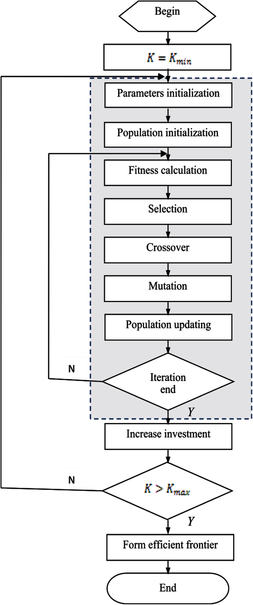
Figure 2: Procedure of optimization based on GA
The proposed GA mainly consists of seven procedures: parameters initialization, population initialization, fitness calculation, selection, crossover, mutation, and population updating. In order to meet the constraint of (2), individuals are limited in the procedure of population initialization, crossover, and mutation. New operators of crossover and mutation are designed to meet the above requirement in the paper.
Parameters initialization: sets the values of population size, chromosome length, probability of crossover, and probability of mutation.
Population initialization: randomly generates a set of individuals whose cost is equal to the set cost value.
Fitness calculation: calculate the fitness value based on the objective value of (2) with the following fitness function:
where
Selection: select the parents of the following generation based on the fitness value of the individual and a selection criterion, e.g., the best known selection criterion, Roulette wheel selection [36].
Crossover: two individuals swap parts of their chromosome with each other at the probability of crossover when the sum of the swapped part is equal.
Mutation: in a single individual, a gene exchanges its value with its neighbor at the probability of mutation.
Population updating: Elitist model is used to update the population, i.e., if the offspring does not have the best individual of the parent, substitute the individual with the lowest fitness value in the offspring for the best individual of the parent. It has been proved that the GA can achieve global convergence with Elitist model in [37,38].
In order to make an intuitive comparison, a simple 12-node distribution system with balance load is firstly simulated and analyzed. Then the IEEE33-node distribution system with unbalanced load is simulated to illustrate the effectiveness and scalability of the proposed method.
4.1 12-Node Distribution System with Balance Load
Fig. 3 shows the single-line diagram of the system, where Node 1 is the substation. The system data including line data and load data can be found in [39].
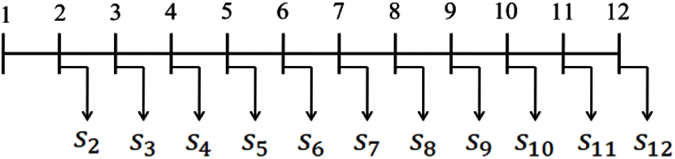
Figure 3: Single-line diagram of the 12-node system
Based on the provided line data and load data, and let
Suppose Node 1 has the measurements from the SCADA system, i.e., voltage magnitude, power flow, and branch current magnitude. The corresponding measure error is set to 1% for voltage magnitude and 3% for power flow and branch current magnitude as in [20,34]. Nodes 2–12 do not have any real measurements and pseudo measurements are used, i.e., Nodes 2–12 have the measurements of power injection (real power and reactive power) with an error of 50% as suggested in [33]. We plan to install PMU on Nodes 2–12, the question is how many PMUs should be used and where to install them. The measure error of PMU is set to 1% as suggested in [6].
To model the uncertainties of the measurement errors and instrument fault, Monte Carlo simulation approach are adopted and the simulation time is 1,000 in the paper. The confidence interval of VaR is set as 95%.
For the parameter setting in GA, the population size is 50, chromosome length is 11, crossover probability is 0.5, mutation probability is 0.001, and the number of iterations is 50. Besides, in order to simplify the calculation, the cost of a PMU is supposed to one unit.
Nine cases are simulated in the paper in order to compare the effect of uncertainties of the measurement errors and instrument fault on the PMU placement, i.e.,
Case 1-1: This is a benchmark. In this case, we do not consider any uncertainties, i.e., we ignore the uncertainty of measurement errors and the possibility of instruments fault.
Case 1-2: Based on Case 1-1, this case considers the uncertainty of measure errors and supposes all the measurement errors are normally distributed.
Case 1-3: Based on Case 1-1, this case considers the uncertainty of measure errors and supposes that real measurement errors are normally distributed and pseudo measurement errors are uniformly distributed.
Case 1-4: Based on Case 1-1, this case considers the possibility of PMU fault with traditional reliability criterion, N-1 criterion, i.e., in each PMU portfolio, 1 PMU is supposed to fault.
Cases 1-5, 6, and 7: Based on Case 1-1, this case considers the possibility of PMU fault and supposes the fault rate of PMU is 0.1, 0.01 and 0.001, respectively.
Cases 1-8 and 9: Based on Case 1-1, this case considers both the uncertainty of measurement error and the possibility of PMU fault. Suppose that all the measurement errors are normally distributed and the fault rate of PMU is 0.01 and 0.1, respectively.
For each case, the efficient frontier is simulated and shown in Figs. 4–12, respectively. The horizontal axis in the figure represents the installation cost of PMU (in order to simplify the calculation, it is assumed that the cost of one PMU is a unit), and the longitudinal ordinate represents the lowest state estimation accuracy that can be achieved under 95% probability. Any point in the efficient frontier corresponds to a PMU portfolio (i.e., a PMU placement plan). Based on the efficient frontier, decision makers can select the appropriate PMU placement plan (i.e., PMU portfolio) based on their subjective judge.
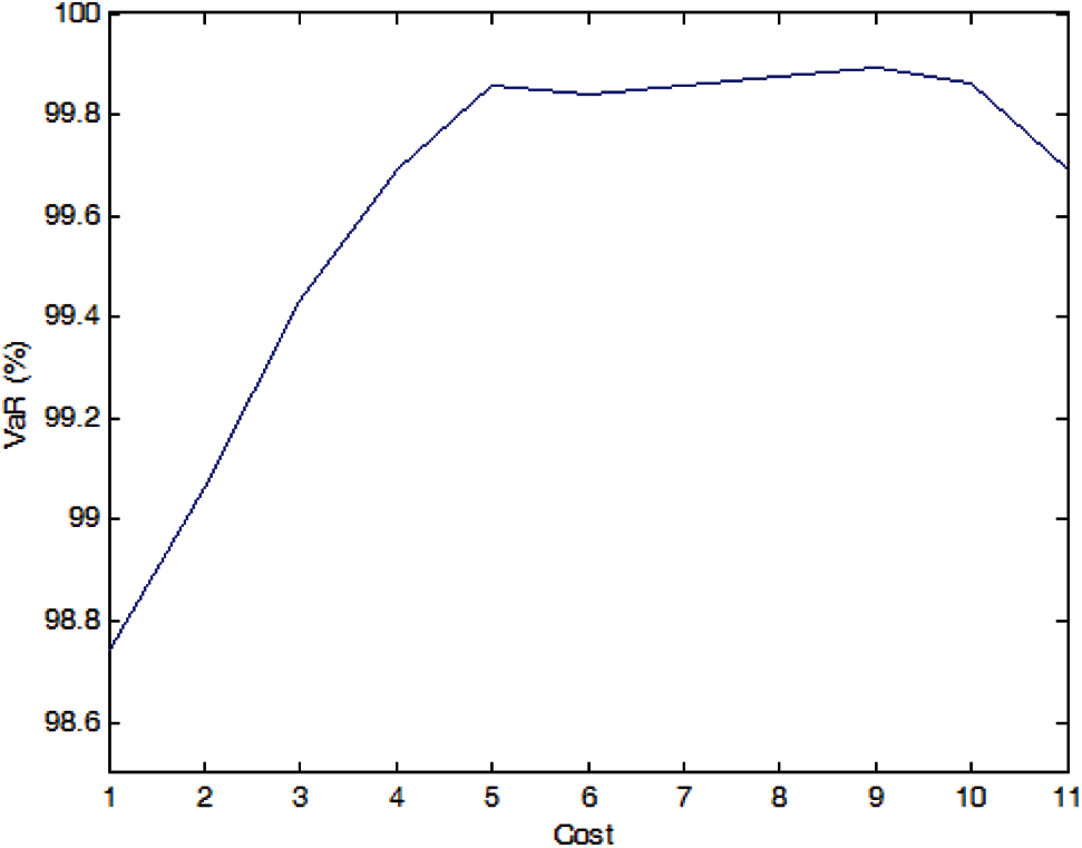
Figure 4: Efficient frontier–Case 1-1
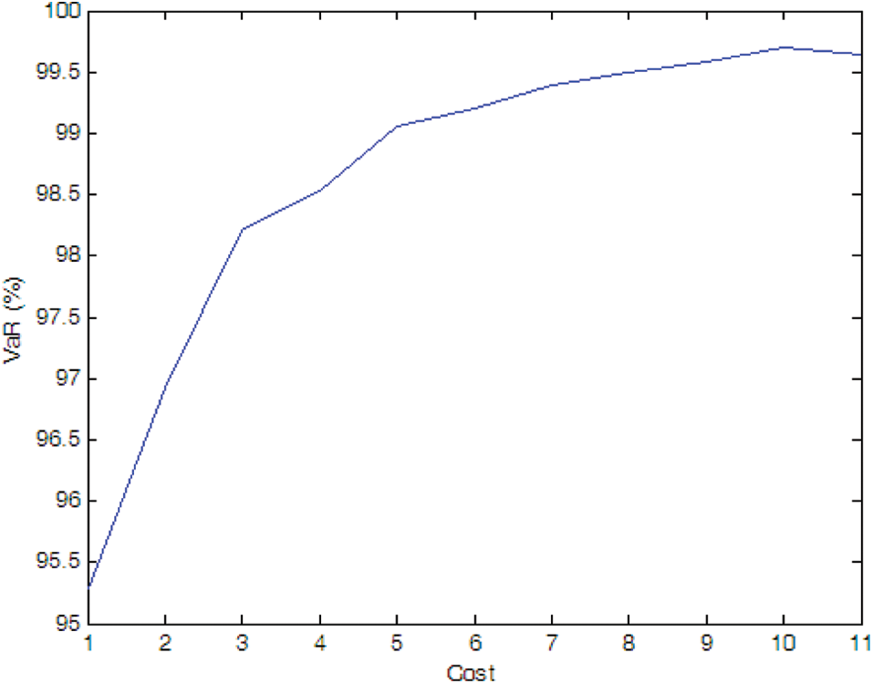
Figure 5: Efficient frontier–Case 1-2
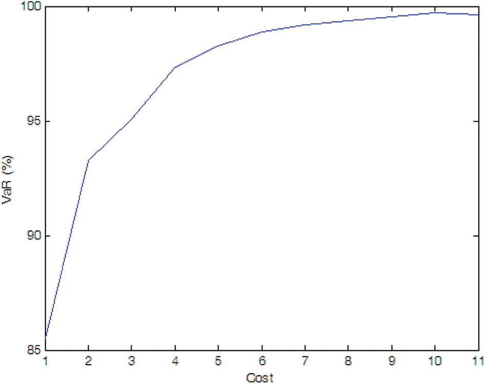
Figure 6: Efficient frontier–Case 1-3
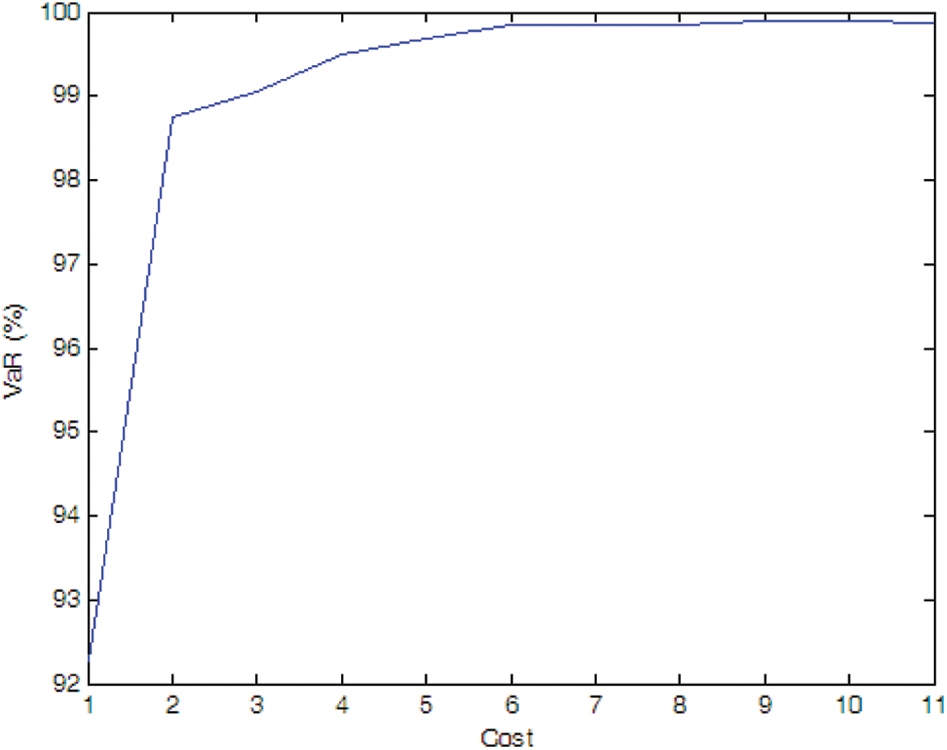
Figure 7: Efficient frontier–Case 1-4
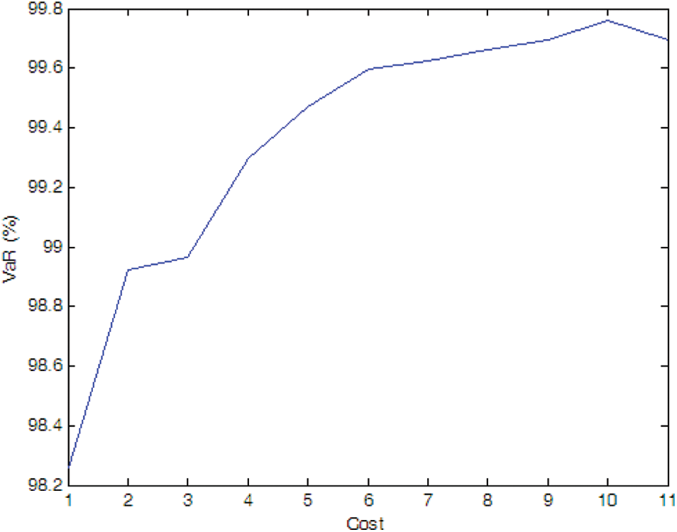
Figure 8: Efficient frontier–Case 1-5
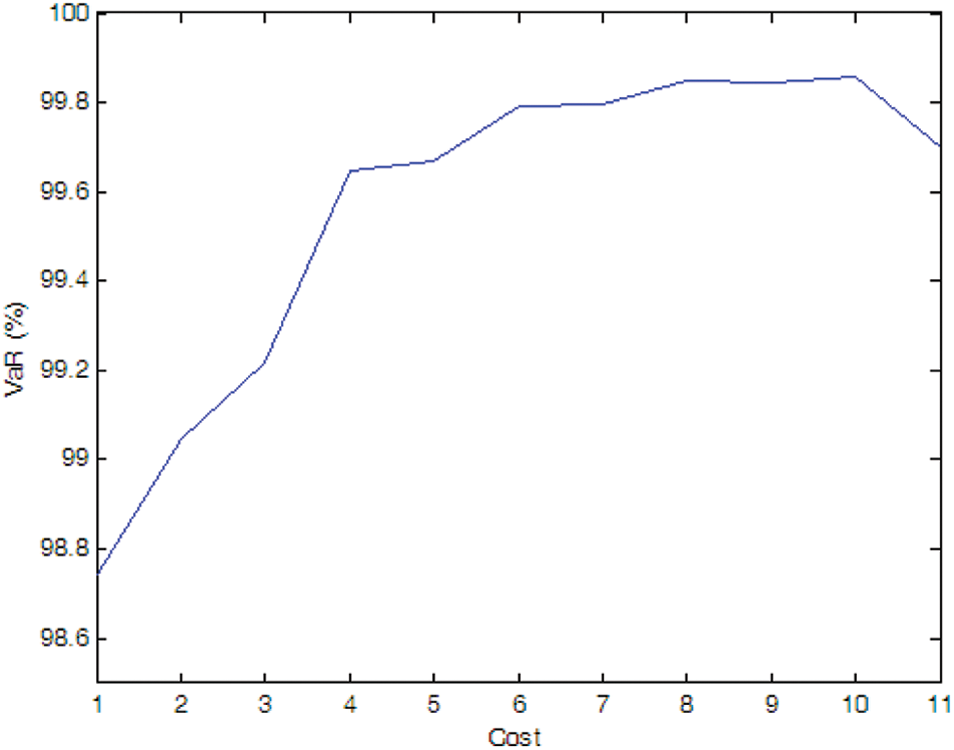
Figure 9: Efficient frontier–Case 1-6
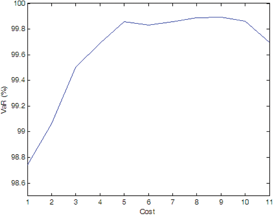
Figure 10: Efficient frontier–Case 1-7
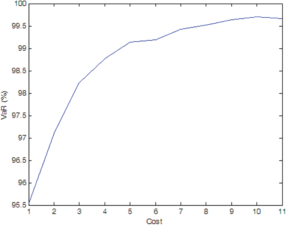
Figure 11: Efficient frontier–Case 1-8

Figure 12: Efficient frontier–Case 1-9
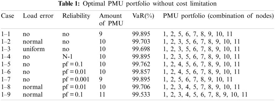
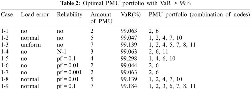
Suppose there is no cost limitation, the optimal PMU portfolio for each case is shown in Table 1. Suppose the expected SE accurate rate is 99%, the optimal PMU portfolio for each case is shown in Table 2.
• General conclusion
If there is no cost limitation, for each case, there is a optimal installation portfolio that maximize the SE accuracy, but the marginal improvement in SE accuracy is obviously reduced when the installation quantity is greater than about 50% of the total potential installation quantity, i.e., 5–6 PMUs in the simulation.
• Effect of measurement uncertainty
If there is no cost limitation, the optimal installation quantity of PMU in Case 1-1, Case 1-2 and Case 1-3 is 9, 10, 10, respectively, and the optimal PMU portfolio in Case 1-2 and Case 1-3 is the same, i.e., the optimal installation site is Nodes 1, 2, 3, 5, 6, 7, 8, 9, 10, and 11. It indicates that more PMUs are needed when we consider the measure uncertainty, but the specific distribution characteristic of the pseudo measurements does not affect the optimal PMU portfolio for a given number of PMU.
If the expected SE accuracy rate is set to 99% with a confidence interval of 95%, the optimal installation quantity of PMU is 2, 5, and 7 for Cases 1-1, 1-2, and 1-3, respectively, which indicates that the SE accuracy is affected by the distribution characteristics of the pseudo measurements and more PMUs are needed to meet a SE accuracy target when the pseudo measurements are not normal distributed (e.g., uniform distribution in the simulation).
• Effect of PMU fault uncertainty
If there is no cost limitation, with the possibility of PMU fault into consideration, more PMUs are needed when we consider the possibility of PMU fault (e.g., Cases 1-4, 1-5, and 1-6) compare to the case without considering PMU fault (i.e., Case 1-1). Of cause, if the fault probability of the PMU is very small (e.g., Case 1-7), the optimal PMU portfolio does not change compared to Case 1-1.
If the expected SE accuracy rate is set to 99%, compared to Case 1-1, more PMUs are needed (e.g., Cases 1-4 and 1-5). If the fault probability of the PMU is smaller (e.g., Cases 1-6 and 1-7), the optimal PMU portfolio does not change compared to Case 1-1.
Simulation results indicate that more PMUs are installed if we consider the possibility of the PMU fault, which is consistent with our intuitive judgment. Furthermore, compared to the N-1 criterion, probability method can more accurately model the effect of PMU fault on the SE. Higher fault probability results in more PMU installed and vice versa.
• Effect of uncertainties of measurement and PMU fault
The optimal PMU portfolio of Case 1-8 is the same as that of Case 1-2 since the fault rate of PMU is quite lower (i.e., 0.01 in Case 1-8). If the fault rate of PMU is higher (i.e., 0.1 in Case 1-9), more PMUs are needed compared to Case 1-2. Tables 1 and 2 demonstrate that the optimal PMU portfolio is mainly affected by the uncertainty of measurement unless the fault rate of PMU is quite high, say, 0.1 in the paper.
4.2 IEEE33-Node Distribution System with Unbalanced Load
The single-line diagram of the IEEE 33-node system is shown in Fig. 13, where Node 0 is the substation. The system data including line data and load data can be found in [40].
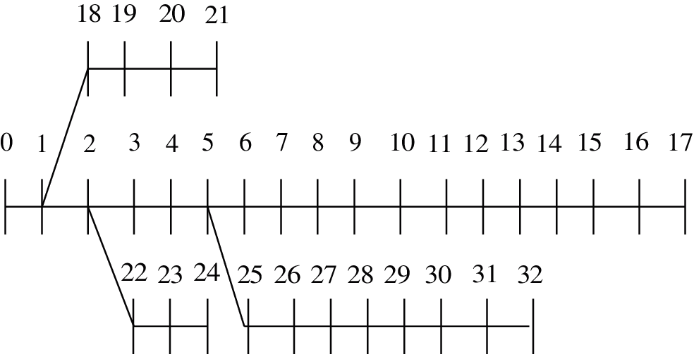
Figure 13: Single-line diagram of the IEEE33-node system
Case 2-1: This case considers the uncertainty of measure errors and supposes all the measurement errors are normally distributed.
Case 2-2: This case considers the uncertainty of measure errors and supposes that real measurement errors are normally distributed and pseudo measurement errors are uniformly distributed.
Cases 2-3 and 4: This case considers the possibility of PMU fault and supposes the fault rate of PMU is 0.1 and 0.01, respectively.
Case 2-5 and 6: This case considers both the uncertainty of measurement error and the possibility of PMU fault. Suppose that all the measurement errors are normally distributed and the fault rate of PMU is 0. 1 and 0.01, respectively.
The simulation results of Cases 2-1 to 2-6 are shown in Figs. 14–19.
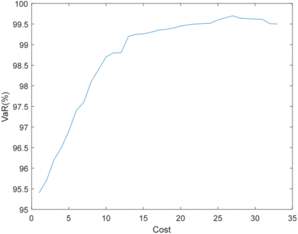
Figure 14: Efficient frontier–Case 2-1
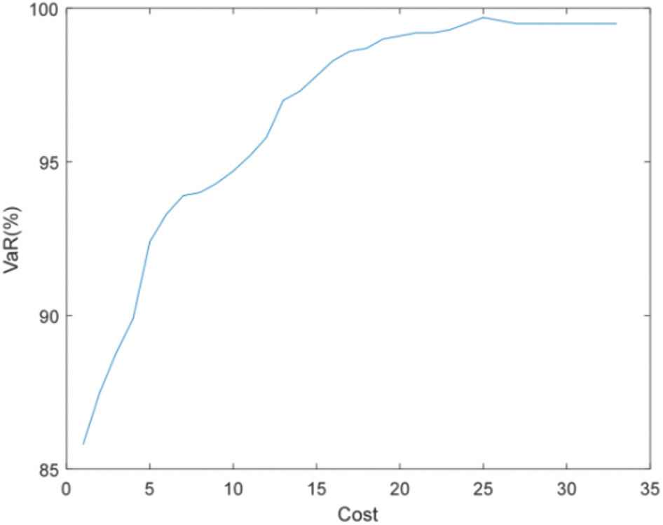
Figure 15: Efficient frontier–Case 2-2
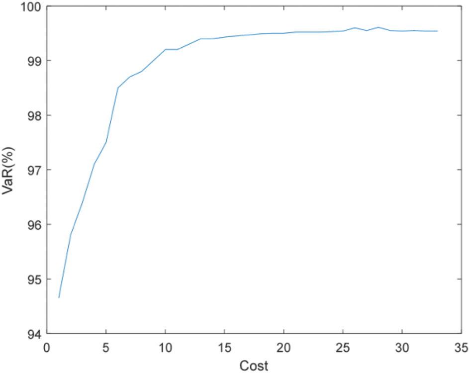
Figure 16: Efficient frontier–Case 2-3
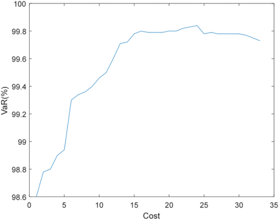
Figure 17: Efficient frontier–Case 2-4
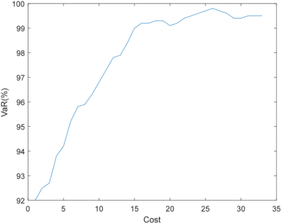
Figure 18: Efficient frontier–Case 2-5
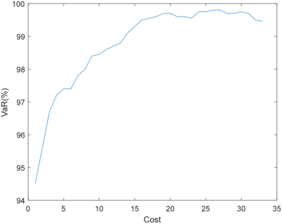
Figure 19: Efficient frontier–Case 2-6
Figs. 14 and 15 show that the accuracy of state estimation is affected by the distribution characteristics of pseudo measurement. When the pseudo measurement obeys the uniform distribution rather than the normal distribution, more PMUs need to be installed to meet the requirements of state estimation accuracy. For example, when the state estimation accuracy is required to be 99%, Case 2-1 needs to install 14 PMUs, while Case 2-2 needs to install 19 PMUs.
Figs. 16 and 17 show that the higher the failure rate of PMU and the more number of units to be installed under the same estimation accuracy requirements. For example, when the accuracy of state estimation is 99%, Case 2-3 (failure rate is 0.1) requires 9 PMUs to be installed, while Case 2-2 (failure rate is 0.01) only needs to install 6 sets.
Compared with Figs. 16 and 18, and Figs. 17 and 19, it can be found that more PMUs need to be installed to meet the accuracy requirements of state estimation when considering both the uncertainty of measurement and the failure rate of PMU. For example, when the accuracy of state estimation is required to be 99%, only 9 PMUs need to be installed when considering PMU failure (failure rate is 0.1), and 16 PMUs need to be installed when considering the uncertainty of measurement at the same time.
Base on the concept of efficient frontier and VaR, this paper proposed a GA based optimization model for optimal placement of PMU (i.e., PMU portfolio). This model considers the measurement uncertainty, statistical characteristics of the pseudo measurements, reliability of the measurement instrument. The reasonability and feasibility of the proposed model is illustrated with a 12-node system and IEEE33-node system. Simulation results indicated that:
i) Uncertainties of measurement error and instrument fault result in more PMU to be installed;
ii) Measurement uncertainty is the main affect factors unless the fault rate of PMU is quite high, and different measurement error distributions have different effects on the optimal configuration of PMU;
iii) The proposed model can make a more reasonable PMU allocation scheme according to the risk preference of decision-maker (given confidence level), compared with the traditional multi-objective weighted optimization and N-1 criterion.
In the future, how to determine the measurement error distribution and the failure rate of PMU will be studied.
Funding Statement: The author Min Liu received the grant of the National Natural Science Foundation of China (http://www.nsfc.gov.cn/) (51967004).
Conflicts of Interest: The author declares that they have no conflicts of interest to report regarding the present study.
1. Gol, M., Abur, A., Galvan, F. (2012). Metrics for success: Performance metrics for power system state estimators and measurement designs. IEEE Power Energy Magazine, 10(5), 50–57. DOI 10.1109/MPE.2012.2205315. [Google Scholar] [CrossRef]
2. Sanchez-Ayala, G., Aguerc, J. R., Elizondo, D., Lelic, M. (2013). Current trends on applications of PMUs in distribution systems. Innovative Smart Grid Technologies, pp. 24–27. Piscataway, NJ, IEEE. [Google Scholar]
3. Alexandra, V. M., Emma, S., Alex, M. (2017). Precision micro-synchrophasors for distribution systems: A summary of applications. IEEE Transactions on Smart Grid, 8(6), 2926–2936. DOI 10.1109/TSG.5165411. [Google Scholar] [CrossRef]
4. Hamed, M., Emma, S., Ed, C. (2018). Distribution synchrophasors. IEEE Power & Energy Magazine, 26–34. DOI 10.1109/MPE.2018.2790818. [Google Scholar] [CrossRef]
5. Liu, J., Tang, J., Ponci, F. (2012). Trade-offs in PMU deployment for state estimation in active distribution grids. IEEE Transactions on Smart Grid, 3(2), 915–924. DOI 10.1109/TSG.2012.2191578. [Google Scholar] [CrossRef]
6. Pau, M., Pegoraro, P. A., Sulis, S. (2013). Efficient branch-current-based distribution system state estimation including synchronized measurements. IEEE Transaction on Instrumentation and Measurement, 62(9), 2419–2429. DOI 10.1109/TIM.2013.2272397. [Google Scholar] [CrossRef]
7. Liu, M. (2017). State estimation in a smart distribution system. HKIE Transactions, 24(1), 1–8. DOI 10.1080/1023697X.2016.1231015. [Google Scholar] [CrossRef]
8. Monticelli, A., Wu, F. F. (1985). Network observability: Identification of observable islands and measurement placement. IEEE Transactions on Power Applied System, 104(5), 1035–1041. [Google Scholar]
9. Gou, B., Abur, A. (2001). An improved measurement placement algorithm for network observability. IEEE Transaction on Power Systems, 16(4), 819–824. DOI 10.1109/59.962432. [Google Scholar] [CrossRef]
10. Li, Q., Cui, T., Weng, Y. (2013). An information-theoretic approach to PMU placement in electric power systems. IEEE Transaction on Smart Grid, 4(1), 446–456. DOI 10.1109/TSG.2012.2228242. [Google Scholar] [CrossRef]
11. Nikolaos, M. M., George, N. K. (2020). Optimal allocation of phasor measurement units considering various contingencies and measurement redundancy. IEEE Transactions on Instrumentation and Measurement, 69(6), 3403–3411. DOI 10.1109/TIM.2019.2932208. [Google Scholar] [CrossRef]
12. Maji, T. K., Acharjee, P. (2020). Operational-based techno-economic PMU installation approach using grey wolf optimisation algorithm (GWOA). IET Generation, Transmission & Distribution, 14(1), 70–78. DOI 10.1049/iet-gtd.2018.7019. [Google Scholar] [CrossRef]
13. Devi, M. M., Geethanjali, M. (2020). Hybrid of genetic algorithm and minimum spanning tree method for optimal PMU placements. Measurement, 154, 1–12. DOI 10.1016/j.measurement.2020.107476. [Google Scholar] [CrossRef]
14. Li, K. (1996). State estimation for power distribution system and measurement impacts. IEEE Transaction on Power Systems, 11(2), 911–916. DOI 10.1109/TPWRS.2009.2016599. [Google Scholar] [CrossRef]
15. Chen, T., Cao, Y., Chen, X., Sun, L., Zhang, J. et al. (2021). Optimal PMU placement approach for power systems considering non-Gaussian measurement noise statistics. International Journal of Electrical Power & Energy Systems, 126, 1–12. DOI 10.1016/j.ijepes.2020.106577. [Google Scholar] [CrossRef]
16. Primadianto, A., Lu, C. N. (2017). A review on distribution system state estimation. IEEE Transactions on Power Systems, 32(5), 3875–3883. DOI 10.1109/TPWRS.2016.2632156. [Google Scholar] [CrossRef]
17. Dehghanpour, K., Wang, Z., Wang, J. (2019). A survey on state estimation techniques and challenges in smart distribution systems. IEEE Transactions on Smart Grid, 10(2), 2312–2322. DOI 10.1109/TSG.5165411. [Google Scholar] [CrossRef]
18. Cano, J. M., Arboleya, P., Ahmed, M. R., Mojumdar, M. R., Orcajo, G. A. (2021). Improving distribution system state estimation with synthetic measurements. International Journal of Electrical Power and Energy Systems, 129, 1–6. DOI 10.1016/j.ijepes.2020.106751. [Google Scholar] [CrossRef]
19. Ghadikolaee, E. T., Kazemi, A., Shayanfar, H. A. (2020). Novel multi-objective phasor measurement unit placement for improved parallel state estimation in distribution network. Applied Energy, 279, 1–14. DOI 10.1016/j.apenergy.2020.115814. [Google Scholar] [CrossRef]
20. Muscas, C., Pilo, F., Pisano, G. (2009). Optimal allocation of multichannel measurement devices for distribution state estimation. IEEE Transaction on Instrumentaiton and Measurement, 58(6), 1929–1937. DOI 10.1109/TIM.2008.2005856. [Google Scholar] [CrossRef]
21. Singh, R., Pal, B. C., Vinter, R. B. (2009). Measurement placement in distribution system state estimation. IEEE Transaction on Power Systems, 24(2), 668–675. DOI 10.1109/TPWRS.2009.2016457. [Google Scholar] [CrossRef]
22. Shafiu, A., Jenkins, N., Strbac, G. (2005). Measurement location for state estimation of distribution networks with generation. IEE Proceedings–Generation, Transmission and Distribution, 152(2), 240–246. DOI 10.1049/ip-gtd:20041226. [Google Scholar] [CrossRef]
23. Singh, R., Pal, B. C., Jabr, R. A. (2011). Meter placement for distribution system state estimation: An ordinal optimization approach. IEEE Transaction on Power Systems, 24(4), 2328–2335. DOI 10.1109/TPWRS.2011.2118771. [Google Scholar] [CrossRef]
24. Pegoraro, P. A., Sulis, S. (2013). Robustness-oriented meter placement for distribution system state estimation in presence of network parameter uncertainty. IEEE Transaction on Instrumentation and Measurement, 62(5), 954–962. DOI 10.1109/TIM.2013.2243502. [Google Scholar] [CrossRef]
25. Liu, J., Ponci, F., Monti, A., Muscas, C., Pegoraro, P. A. et al. (2014). Optimal meter placement for roubust measurement systems in active distribution grids. IEEE Transaction on Instrumentation and Measurement, 63(5), 1096–1105. DOI 10.1109/TIM.2013.2295657. [Google Scholar] [CrossRef]
26. Celik, M. K., Liu, W. H. E. (1995). An incremental measurement placement algorithm for state estimation. IEEE Transaction on Power Systems, 10(3), 1698–1703. DOI 10.1109/59.466471. [Google Scholar] [CrossRef]
27. Prasad, S., Kumar, D. M. V. (2018). Trade-offs in PMU and IED deployment for active distribution state estimation using multi-objective evolutionary algorithm. IEEE Transactions on Instrumentation and Measurement, 67(6), 1298–1307. DOI 10.1109/TIM.2018.2792890. [Google Scholar] [CrossRef]
28. Liu, J., Tang, J., Ponci, F. (2012). Trade-offs in PMU deployment for state estimation in active distribution grids. IEEE Transaction on Smart Grid, 3(2), 915–924. DOI 10.1109/TSG.2012.2191578. [Google Scholar] [CrossRef]
29. Celli, G., Pegoraro, P. A., Pilo, F. (2014). DMS cyberphysical simulation for assessing the impact of state estimation and communication media in smart grid operation. IEEE Transaction on Power System, 29(5), 2436–2446. DOI 10.1109/TPWRS.2014.2301639. [Google Scholar] [CrossRef]
30. Bodie, Z., Kane, A., Marcus, A. J. (1999). Investments, 4th ed. Chicago: Irwin/McGraw-Hill. [Google Scholar]
31. Wu, F. (1990). Power system state estimation: A survey. Electrical Power & Energy Systems, 12(2), 80–87. DOI 10.1016/0142-0615(90)90003-T. [Google Scholar] [CrossRef]
32. Jorion, P. (1997). Value at risk. New York: McGraw-Hill. [Google Scholar]
33. Singh, R., Pal, B. C., Jabr, R. A. (2009). Choice of estimator for distribution system state estimation. IET Generation, Transmission, and Distribution, 3, 666–678. DOI 10.1049/iet-gtd.2008.0485. [Google Scholar] [CrossRef]
34. Abur, A., Exposito, A. G. (2004). Power system state estimation: Theory and implementation. New York: Marcel Dekker. [Google Scholar]
35. Gen, M., Cheng, R. (2000). Genetic algorithms and engineering optimization. New York: John Wiley & Sons. [Google Scholar]
36. Holland, J. (1992). Adaptation in natural and artificial systems. Cambridge, MA: MIT Press. [Google Scholar]
37. Eiben, A. E., Aaris, E. H., Hee, K. M. V. (1991). Global convergence of genetic algorithms: An infinite markov chain analysis. In: Parallel problem solving from nature, pp. 4–12. Berlin: Springer-Verlag. [Google Scholar]
38. David, B. F. (1995). Evolutionary computation-toward a new philosophy of machine intelligence. Piscataway, NJ: IEEE Press. [Google Scholar]
39. Das, D., Nagi, H. S., Kothari, D. P. (1994). Novel method for solving radial distribution networks. Proceeding of IEEE Generation, Transmission and Distribution, 141(4), 291–298. DOI 10.1049/ip-gtd:19949966. [Google Scholar] [CrossRef]
40. Baran, M. E., Wu, F. F. (1989). Network reconfiguration in distribution systems for loss reduction and load balancing. IEEE Transaction on Power Delivery, 4(2), 1401–1407. DOI 10.1109/61.25627. [Google Scholar] [CrossRef]
 | This work is licensed under a Creative Commons Attribution 4.0 International License, which permits unrestricted use, distribution, and reproduction in any medium, provided the original work is properly cited. |