Energy Engineering

DOI: 10.32604/ee.2022.017703

ARTICLE

Identification and Classification of Multiple Power Quality Disturbances Using a Parallel Algorithm and Decision Rules

Nagendra Kumar Swarnkar1, Om Prakash Mahela2, Baseem Khan3,* and Mahendra Lalwani1

1Department of Electrical Engineering, Rajasthan Technical University, Kota, India
2Power System Planning Division, Rajasthan Rajya Vidyut Prasaran Nigam Limited, Jaipur, India
3Department of Electrical and Computer Engineering, Hawassa University, Awassa, Ethiopia
*Corresponding Author: Baseem Khan. Email: baseem.khan04@gmail.com
Received: 31 May 2021; Accepted: 23 July 2021

1  Introduction

Equipment used in industrial processes is sensitive to the quality of power. Hence, bad or poor power quality (PQ) affects the efficiency of industrial production and the quality of the finished products [1]. Hence, PQ is identified as a major challenge for the utilities and customers [2]. Non-linear loads, electronic appliances, large and random changes in the utility grid, and the uncertain and unpredictability of renewable energy (RE) generation are major sources of PQ disturbances [3]. PQ disturbances cause blackouts, sub-network disconnection, and dynamic propagation of disturbances [4]. These disturbances may be single-stage PQ disturbances where one disturbance is an incident [5].

1.1 Related Research Works

This section details the research work reported in the literature related to the detection and classification of PQ disturbances, with emphasis on multiple PQ disturbances. In [6], the authors designed a hybrid technique based on the concept of deep learning, combining the 1-Dimensional (1-D) power signals and 2-Dimensional (2-D) signal images to identify and classify the PQ disturbances. This method has high classification accuracy and moderate complexity of computation. This method is implemented by combining the structure of a 1-D convolutional neural network (CNN) with the structure of a 2-D CNN to compute the features. These features are classified by the application of a fully connected layer. The voltage signal with PQ disturbance is processed using 1-D CNN to convert signals into images. These images are processed using 2-D CNN. Finally, the 1-D CNN output vector and 2-D CNN output vector are combined to classify the PQ disturbances using the fully connected layer. A hybrid algorithm using different features computed using the signal processing techniques for detection and categorization of MPQ disturbances is available in [7]. The voltage signal with PQ disturbance is processed by the application of ST to compute the output matrix. The summation of absolute values of every column of this matrix is computed and assigned the name ST-index. Further, the same voltage signal is also processed by the application of HT and absolute values of output are computed, which is assigned the name H-index. The ST-index and H-index are combined to compute the power quality index (PQI), which is an effective way to recognize all types of MPQ disturbances. The peak magnitude of this index is considered as an input for classifying the MPQ disturbances. This method has the demerits of not locating the MPQ disturbances, relatively high computational complexity, and low accuracy of 97%. In [8], the authors designed a hybrid method based on the concept of deep learning to classify the MPQ disturbances using the variations of single-stage PQ disturbances. Various sub-components of MPQ signals are computed according to signal characteristics and instantaneous energies from these subcomponents are computed which are considered as input to the deep learning (DL). Cycles of deep learning are designed in accordance with the quantum of instantaneous energy of a signal, which represents a specific feature of a MPQ disturbance. Techniques effectively classify the MPQ disturbances with high accuracy. A hybrid technique applying FL and particle swarm optimization (PSO) designed to identify and classify the PQ disturbances of single and multiple natures is reported in [9]. This technique computes the eight features from the waveform of a signal with PQ disturbance, which includes the fundamental component, phase angle shift, total harmonic distortions (THD), number of maximums of the absolute value of wavelet coefficients, energy of the wavelet coefficients, number of zero-crossings of the missing voltage, lower harmonic distortion, and number of peaks of root mean square (RMS) value. These features are extracted using the parameters computed using FT and WT based processing of signals. These features are utilized to classify the disturbances using a fuzzy system. This technique is efficient for identifying various single and multiple PQ disturbances under noisy conditions. In [10], the authors designed a method for detecting and classifying MPQ disturbances by the application of HT and RBDT. The voltage signal with MPQ disturbance is processed using the HT and absolute values of output are computed, which is assigned the name H-index. Four features, namely median, kurtosis, standard deviation, and variance, are extracted from the H-index. These features are considered as input to the rule based decision tree to classify the disturbances. This method has the disadvantage of high computational time. A real-time analysis of single and multiple PQ disturbances using amplitude and frequency demodulation concepts is introduced by the authors in [11]. The demodulation concept is utilized for separating the various patterns of single/multiple PQ events. The music harmonics algorithm is implemented for detecting the availability of harmonics of various natures, which includes transient, sag, swell, and their hybrid combinations. A Fuzzy classifier is utilized to classify the PQ events with the help of a knowledge base derived from the amplitude demodulation, frequency demodulation, and MUSIC harmonic algorithm. The PQ algorithm effectively identifies the PQ events having the nature of transients, sag, swell, and harmonics. Classification of disturbances is achieved using the fuzzy classifier. In [12], the authors introduced a technique using multidimensional analysis, higher-order statistics, and a neuro-tree based classifier to detect and classify single and multiple PQ disturbances. The signal data has been acquired using a field programmable gate array (FPGA). The Notch filter is used to filter the data, which is then divided into two categories: the original signal and the error components. The peripheral component interconnects (PCI) bus is used to transfer this data to the real-time processor, where it is applied to the original signal. If MPQ disturbance is absent, then the process ends here. The presence of MPQ disturbance is identified by writing the filtered and original signal data and transferring them via network stream to a remote computer to classify the disturbances using higher order statistics and RMS values method effectively classified the 20 events of single and multiple PQ disturbances with accuracy greater than 97%. The performance of the method is decreased for higher noise levels. In [13], the authors designed a technique using the time–frequency resolution characteristic of ST for the detection of PQ disturbances. Classification of PQ disturbances is achieved using SVM. This technique requires fewer features compared to the WT-based techniques. It has the merit of requiring less computational time from the processor. A voting approach using DWT and an ensemble classification technique is designed by the authors in [14]. The method is implemented in steps, including data collection, feature extraction, first-level classification (base classifiers), and second-level classification (ensemble with voting approach). This technique has been effectively implemented to classify the PQ disturbances associated with a micro-grid with solar photovoltaic (PV) energy integration with an accuracy of 100%. A PQ detection technique using fast variants of the discrete ST (FDST) effective for extracting the time-localized spectral characteristics of non-stationary signals is introduced in [15]. A window function of general nature is designed to improve the concentration of energy in a time–frequency (TF) distribution of signals. Features required to classify the MPQ disturbances are extracted from the time–frequency distribution of signals. A decision tree (DT) is constructed which works automatically for the selection of the optimal set of features using a specified optimal criteria to extract the decision rules which are used to identify the type of PQ disturbance. It improved the energy concentration of the time–frequency (TF) distribution of signals with PQ disturbances. It is effective to identify the various PQ disturbances with noise levels of 30 dB SNR. However, performance is reduced for noise levels higher than 30 dB SNR. A technique based on the combined use of ST and decision tree (DT) for identification and classification of different classes of PQ disturbances is reported in [16]. A moving, localizing, and scalable Gaussian window is used to design ST for computing five statistical features of PQ disturbances, which include the high frequency of oscillatory transient (OT), differentiation between stationary and non-stationary nature of the signal, oscillations of voltage magnitude near average value, availability of harmonics with the signal, and the RMS voltage at the internal period of sag, swell, or interruption. These features are classified into nine groups using DT to identify the PQ events of different natures. This algorithm is effective for automatic identification of PQ disturbances in real-time scenarios. In [17], the authors designed a technique based on probabilistic intelligence for recognition of PQ events associated with a micro-grid (MG). The Discrete Wavelet Transform (DWT) is used to process signals with multiple PQ disturbances in order to extract features. These features are utilized for training the computational intelligence-based classifiers based on Support Vector Machine (SVM) and Naive Bayes (NB). It is established that the multiple PQD events associated with the network of MG have been classified with 100% accuracy. An automated technique for identification and classification of multiple PQ disturbances supported by empirical WT based adaptive filtering and a multiclass SVM is introduced in [18]. The Empirical WT adaptive filtering technique is used for feature extraction and classification is achieved using SVM. The proposed technique effectively identified the eight single-nature PQ disturbances and seven multiple PQ disturbances with high recognition efficiency and low computational time.

1.2 Research Contribution

This is inferred from detailed analysis of PQ identification and classification techniques discussed in the above paragraph, that existing methods effectively identify the PQ disturbances of a single nature with high accuracy, greater than 98%, whereas the efficiency reduces for multiple-nature PQ disturbances. Further, the efficiency of these methods decreases in the presence of high noise levels. Additionally, it is also established that the existing methods require a large number of features (7 to 10 or more) for classification of multiple PQ disturbances. These research gaps can be mitigated using the hybrid combination of the various signal processing methods. This will help in the identification and classification of MPQ disturbances with an accuracy higher than 98% even in the presence of noise at higher levels using only four features. Hence, this paper has considered carrying out further research using a hybrid combination of ST, HT, and decision rules to design a hybrid algorithm to identify and categorize MPQ disturbances. The main contributions of this manuscript are summarized below:

•   A hybrid algorithm using the parallel approach supported by ST and HT with decision rules is investigated to identify and classify the MPQ disturbances.

•   An MPQ identification index is proposed which has different patterns for various types of MPQ disturbances. Hence, it effectively identifies all the MPQ disturbances.

•   The MPQ time location index is computed using the features extracted from the voltage signal with an associated MPQ disturbance, applying the ST and HT for time location of MPQ disturbances. It effectively identifies the initiation and end of the MPQ disturbances and thereby locates the MPQ events.

•   The MPQ algorithm is effective in classifying the MPQ events using decision rules with the help of four features in both the noise-free and noisy environments.

•   Performance of the technique using ST and HT with RBDT is better compared to ST and RBDT technique in terms of accuracy of classification of MPQ disturbances.

1.3 Organization of Contents

The paper is organized into seven sections. The first section, describes the review of literature, research gaps, and contribution of this manuscript. The formulation of MPQ disturbances is described in the second section. All the steps of the proposed algorithm are detailed in the third section. The results used to identify the MPQ disturbances and their discussions are included in Section 4. This section also discussed the results for the classification of MPQ disturbances. Performance estimation of the algorithm is illustrated in Section 5. A comparative study of this proposed algorithm with the algorithm reported in the literature is also included in this section. Validation of the performance of the algorithm to identify the MPQ disturbances in the real time scenario has been discussed in Section 6. Finally, research is concluded in Section 7 of the manuscript.

2  Generation of Multiple PQ Disturbance

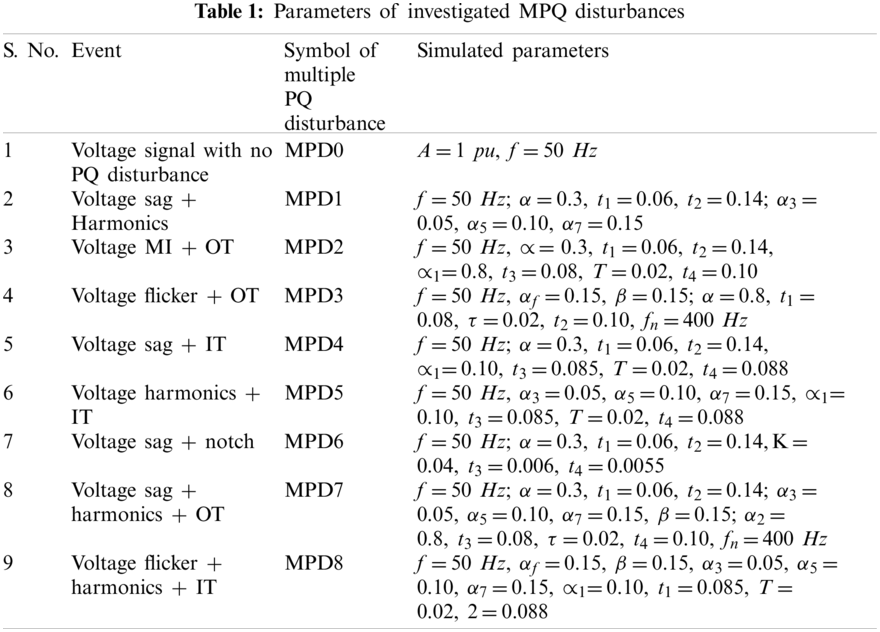
Multiple PQ disturbances have been formulated as per standards defined in the IEEE-1159 standard using mathematical formulations reported in [19,20]. Sine wave without any MPQ disturbance is considered as reference for analysis of the MPQ disturbances. Various parameters used to design the MPQ disturbances are provided in Table 1. Mathematical formulation of investigated multiple PQ (MPQ) disturbances are detailed below where symbols are defined as, A: amplitude of voltage, f: frequency (it is considered equal to 50 Hz for all disturbances), V: instantaneous value of voltage, T: time period, ω: angular frequency, τ: time constant, u(t): unit step function of voltage, K: reduced amplitude of voltage used to define notch, t: instantaneous time, α: reduced amplitude of voltage used to define MPQ disturbances other than notch and spike, e: exponential function, n: number of notches, sin: sine trigonometric function, and sign: signum function.

1. Voltage signal having sinusoidal nature [19].

V(t)=Asin⁡(ωt) (1)

2. Voltage with sag and harmonics multiple PQ disturbance [20].

V(t)=[1−α(u(t−t1)−u(t−t2))]sin⁡(ωt)+α3sin⁡(ωt)+α5sin⁡(ωt)+α7sin⁡(ωt) (2)

3. Voltage with momentary interruption (MI) and oscillatory transient (OT) multiple PQ disturbance [20].

V(t)=[1−α(u(t−t1)−u(t−t2))]sin⁡(ωt)+α1e(t−t3)τsin⁡(ωn(t−t3)(u(t4−u(t3))) (3)

4. Voltage with flicker and OT multiple PQ disturbance [20].

V(t)=(1+αfsin⁡(βωt))sin⁡(ωt)+αe(t−t1)τsin⁡(ωn(t−t1)(u(t2−u(t1))) (4)

5. Voltage sag and impulsive transient (IT) multiple PQ disturbance [20].

V(t)=[1−α(u(t−t1)−u(t−t2))]sin⁡(ωt)+α1e(t−t3)τ−α1e(t−t3)τ(u(t4−u(t3))) (5)

6. Voltage signal with harmonics and IT multiple PQ disturbance [20].

V(t)=sin⁡(ωt)+α3sin⁡(ωt)+α5sin⁡(ωt)+α7sin⁡(ωt)+αe(t−t1)τ−αe(t−t1)τ(u(t2−u(t1))) (6)

7. Voltage signal with sag and notch multiple PQ disturbance [20].

V(t)=[1−α(u(t−t1)−u(t−t2))]sin⁡(ωt)+−sign(sin⁡(ωt))×[∑n=09K×{u(t−(t3+0.02n))−u(t−(t4+0.02n))}] (7)

8. Voltage with sag, harmonics and OT multiple PQ disturbance [20].

V(t)=[1−α(u(t−t1)−u(t−t2))]sin⁡(ωt)+α3sin⁡(ωt)+α5sin⁡(ωt)+α7sin⁡(ωt)+α2e(t−t3)τsin⁡(ωn(t−t3)(u(t4−u(t3))) (8)

9. Voltage signal with flicker, harmonics and IT multiple PQ disturbance [20].

V(t)=(1+αfsin⁡(βωt))sin⁡(ωt)+α3sin⁡(ωt)+α5sin⁡(ωt)+α7sin⁡(ωt)+αe(t−t1)τ−αe(t−t1)τ(u(t2−u(t1))) (9)

3  PQ Identification and Classification Algorithm

Hybrid algorithm used to identify and classify the MPQ disturbances is described in Fig. 1. Different steps of the algorithm and mathematical computations are described in below detailed subsections.

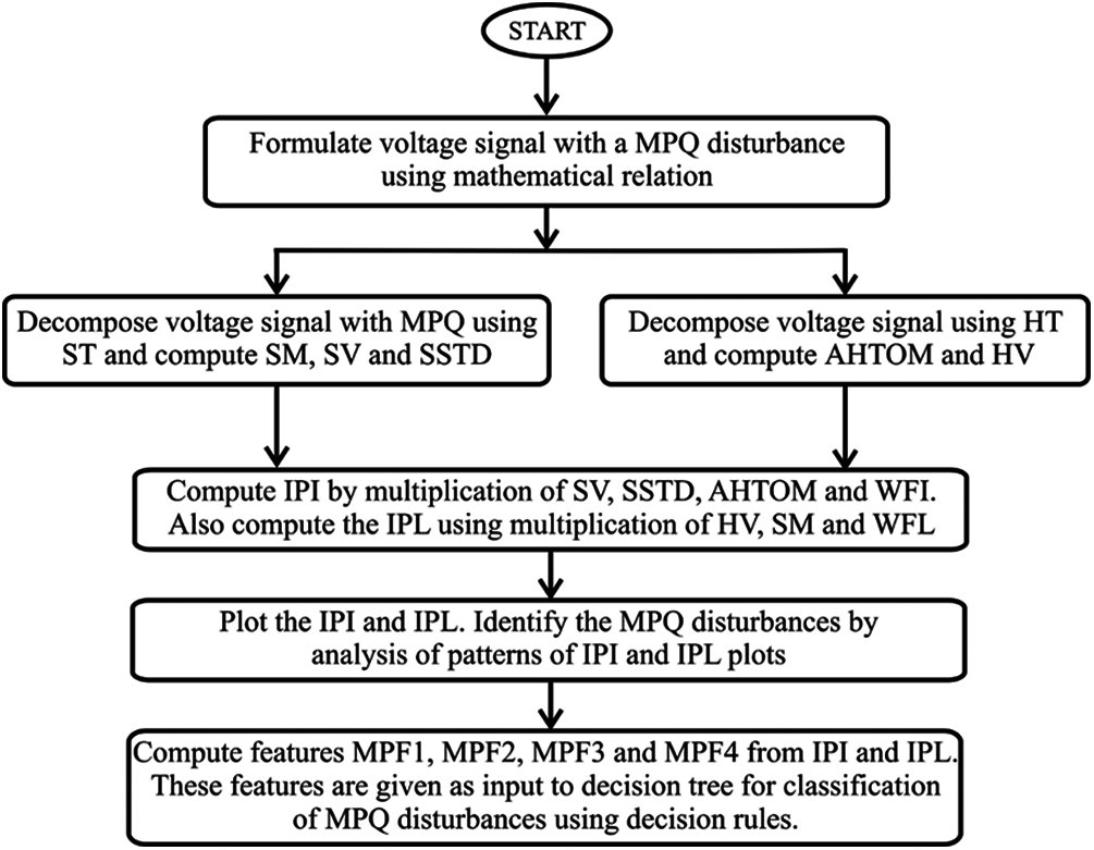
Figure 1: Hybrid algorithm for recognition of MPQ disturbances

3.1 Processing of Voltage Signal with MPQ Disturbance Using ST

Different features are computed by processing the voltage having an associated MPQ disturbance using ST as described below:

•   Process voltage signal with a MPQ disturbance (v) using ST and compute absolute values output matrix (ASTOM).

ASTOM=abs(stran(v)) (10)

The MATLAB command abs is used to compute the absolute value of data series. The function stran is used for the detailed mathematical formulation of ST used in the study which are available in [21,22] and a brief description is presented here. The voltage signal with MPQ disturbance (v(t)) is decomposed using the short time Fourier transform (STFT), and output (ST) is computed as described below [21]:

STI(τ,f)=∫−∞+∞i(t)g(τ−t)e−j2πftdt (11)

where t and f indicate the spectral localization time and Fourier frequency respectively, and g(t) represents the window function. Following Gaussian function (g(t)) is used in the above equation to compute the ST based decomposition of v(t) [21]:

g(t)=|f|2πe−f2t22 (12)

Hence, the output matrix (which is complex in nature) of the ST based decomposition of voltage signal with MPQ disturbances (STM) can be given by the following relation [22].

STOM(τ,f)=∫−∞+∞i(t)|f|2πe−f2(τ−t)22e−j2πftdt (13)

The STOM matrix is a complex valued matrix. Absolute values matrix is computed by taking the absolute values of every element.

ASTOM=abs(STOM) (14)

Matrix ASTOM is used to extract the information of frequency and amplitude of the voltage signal with MPQ disturbance and used for computation of various features utilized for identification of MPQ disturbances.

•   Compute median of ASTOM matrix (SM) using the below detailed relation.

SM=median(ASTOM) (15)

Here, MATLAB command ‘median’ is inbuild command of software and used to compute median of the data series.

•   Compute variance of ASTOM matrix (SV) using the below detailed relation.

SV=var(ASTOM) (16)

Here, MATLAB command ‘var’ is inbuild command of software and used to compute variance of the data series.

•   Compute standard deviation of ASTOM matrix (SSTD) using the below detailed relation.

SSTD=std(ASTOM) (17)

Here, MATLAB command ‘std’ is inbuild command of software and used to compute standard deviation of the data series.

3.2 Processing of Voltage Signal with MPQ Disturbance Using HT

Different features are computed by processing the voltage with an associated MPQ disturbance applying HT as described below:

•   Process voltage with a MPQ disturbance (v) applying HT and compute absolute values output matrix (AHTOM).

AHTOM=abs(hilbert(v)) (18)

The function hilbert is used for the detailed mathematical formulation of HT used in the study which are available in [23]. The HT supported decomposition of voltage signals with MPQ disturbance can be computed using the below detailed relation [23].

HT(v(t))=1πPV∫−∞+∞v(τ)t−τdτ (19)

Here, PV: Cauchy’s principle value integral, t: time, and τ: time period.

•   Compute variance of ASTOM matrix using the below detailed relation.

HV=var(ASTOM) (20)

3.3 MPQ Identification Index

An index is computed using the features extracted from the voltage signal with an associated MPQ disturbance applying the ST and HT for identification of MPQ disturbances which is given the name IPI. Computation of IPI is detailed below:

IPI=SV×SSTD×AHTOM×WFI (21)

Here, AHTOM is a row matrix which is directly used for computation of IPI and WFI is the weight factor used for identification of MPQ disturbances. WFI equal to 104 is considered for this study. The relation of IPI index is fixed after testing on 80 data set of each disturbance which is obtained by variation of parameters such as amplitude, time interval of disturbance, frequency, combination of various PQ disturbances, etc. Further, various features have also been considered using the statistical formulations and it is established that combination of SV, SSTD and AHTOM gives the best results in terms of maximum efficiency.

3.4 MPQ Time Location Index

An index is computed using the features extracted from the voltage signal with an associated MPQ disturbances applying the ST and HT for time location of MPQ disturbances which is given the name IPL. Computation of IPL is detailed below:

IPL=HV×SM×WFL (22)

Here, WFL is the weight factor used for time location of MPQ disturbances. WFL equal to 104 is considered for this study. The relation of IPL index is fixed after testing on 80 data set of disturbances, which has the magnitude and transient components. This data set is obtained by variation of parameters such as amplitude, time interval of disturbance, frequency, combination of various PQ disturbances, etc. Further, various features have also been considered using the statistical formulations and it is established that combination of HV, and SM gives the best results in terms of effective time location of disturbances.

3.5 Classification of MPQ Disturbances

The MPQ disturbances have been classified using the decision rules which are derived from the features (MPF1 to MPF4) computed from the IPI and IPL as detailed below:

MPF1: Covariance of IPI

MPF1=cov(IPI) (23)

MPF2: Summation of all elements of IPI

MPF2=sum(IPI) (24)

MPF3: Covariance of IPL

MPF3=cov(IPL) (25)

MPF4: Summation of all elements of IPL

MPF4=sum(IPL) (26)

The MATLAB commands ‘cov’ and ‘sum’ are the inbuilt commands of the software which contains the necessary equations to compute the covariance and summation of data series respectively. The decision rules arrange the data in structure of a tree. Prediction starts from the root node of the tree and end decision is represented by the leaf nodes of the tree. This is achieved by a set of decision rules. Decision rules effectively classify the MPQ disturbances at fast rate and involves the low complexity and computational time [24].

4  Identification of Multiple PQ Disturbance: Simulation Results and Discussion

The results to identify and classify the multiple PQ disturbances and their discussion are elaborated in this section. MPQ disturbances with multiplicity two and three are described in this section.

4.1 Voltage Signal with Sinusoidal Nature

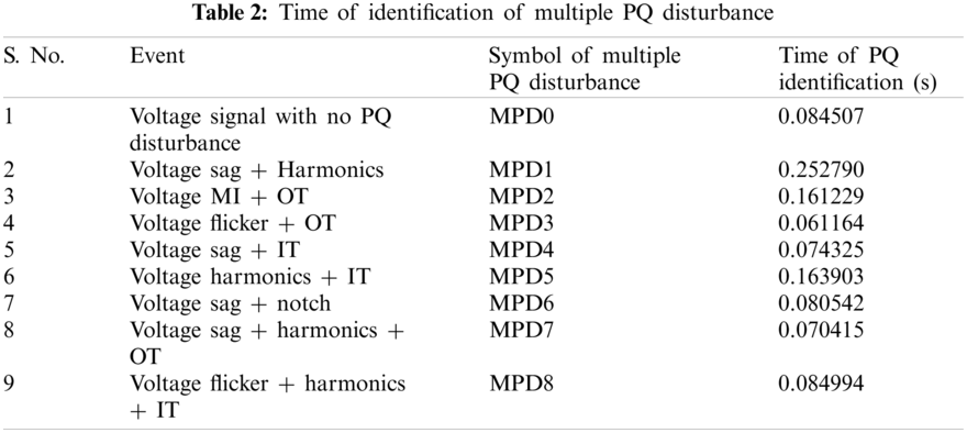
A voltage signal without any MPQ disturbance is simulated by modelling the expressions described in Section 2 using the MATLAB software and elaborated in Fig. 2a. Voltage is decomposed using the ST and HT to compute the MPQ identification index (IPI) and MPQ time location index (IPL). The IPI and IPL are elaborated in Figs. 2b and 2c, respectively. The time of processing the voltage signal using the designed algorithm is provided in Table 2. Fig. 2a details that the nature of the voltage waveform is pure sinusoidal over the complete time range, which indicates that any MPQ event is not associated with voltage. It is perceived from Fig. 2b that the plot of IPI is a straight line over the complete time range. Further, the magnitude of the IPL plot is near to zero over the complete time range, as depicted in Fig. 2c. Hence, plots of IPI and IPL indicate that there is no disturbance in voltage and the pure sinusoidal nature of the waveform is maintained over the complete time range of analysis. Further, the time of analysis is small and equals 0.084507 s.

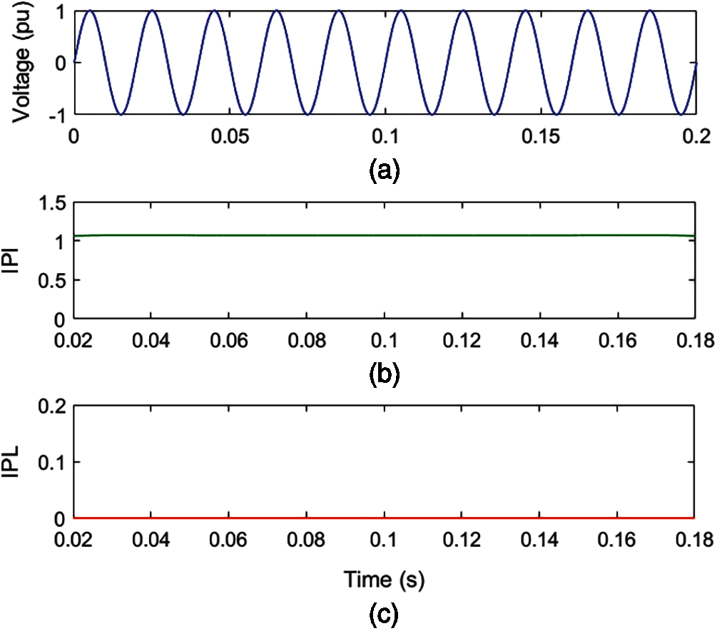
Figure 2: Voltage signal having sinusoidal nature (a) Voltage (b) MPQ identification index (c) IPL

4.2 Voltage Signal with Sag and Harmonics Multiple PQ Disturbance

A voltage signal with an associated MPQ disturbance of degree two multiplicities, including sag and harmonics, is simulated using a mathematical formulation, as shown in Fig. 3a. Voltage is decomposed using ST and HT to compute the MPQ identification index (IPI) and MPQ time location index (IPL). The IPI and IPL for MPQ disturbance of sag and harmonics are elaborated in Figs. 3b and 3c, respectively. The time of processing the voltage signal with MPQ disturbance with sag and harmonics using the proposed algorithm is provided in Table 2.

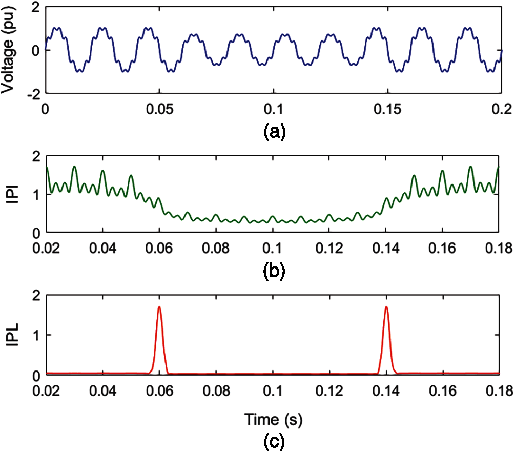
Figure 3: Voltage with sag and harmonics multiple PQ disturbance (a) Voltage (b) MPQ identification index (c) IPL

Fig. 3a details that voltage magnitude decreases for periods of 0.06 to 0.14 s and ripples are superimposed over the voltage signal. It is perceived from Fig. 3b that the magnitude of the IPI plot has reduced from 0.06 to 0.14 s, which indicates the incidence of voltage sag. Further, low-magnitude ripples are associated over the entire time range. This indicates the presence of harmonic components. It is evaluated from Fig. 3c that there are peaks of high magnitude at instants of 0.06 and 0.14 s which indicate the availability of incidence and end of the sag disturbance. Hence, plots of IPI and IPL indicate that there is a MPQ disturbance consisting of sag and harmonics associated with voltage. Further, the time of analysis of the MPQ disturbance, comprised of sag and harmonics, is small and equal to 0.252790 s.

In order to investigate the impact of noise on the efficacy of the algorithm, a voltage signal with an associated MPQ disturbance of two multiplicities comprising of sag and harmonics is simulated using a mathematical formulation. A noise of level 20 dB SNR is superimposed on this voltage signal, which is elaborated in Fig. 4a. Addition of 20 dB SNR noise to the voltage signal is achieved using the awgn command of MATLAB. This awgn is an inbuilt command of MATLAB, which contains all the necessary equations to generate the noise. A voltage signal (v) with MPQ disturbance of sag and harmonics is generated in MATLAB using the expression (2), and noise of 20 dB SNR is added using the following command.

v=awgn(v,20) (27)

Voltage with MPQ disturbance and noise is decomposed by applying ST and HT to compute the MPQ identification index (IPI) and MPQ time location index (IPL). The IPI and IPL for MPQ disturbance of sag and harmonics in a noisy environment are elaborated in Figs. 4b and 4c, respectively.

Fig. 4a details that voltage magnitude decreases during a time interval from 0.06 to 0.14 s and ripples are superimposed on the voltage signal. It is perceived from Fig. 4b that the magnitude of the IPI plot has reduced from 0.06 to 0.14 s, which indicates the incidence of the voltage sag. Further, low-magnitude ripples are associated, which indicate the presence of harmonic components. It is evaluated from Fig. 4c that peaks of high magnitude at times of 0.06 and 0.14 s are present, which indicates the availability of incidence and end of the sag disturbance. However, low-magnitude ripples over the complete time range indicate the availability of noise. Hence, plots of IPI and IPL indicate that there is a MPQ disturbance consisting of sag and harmonics with voltage signal during a noisy environment of 20 dB SNR.

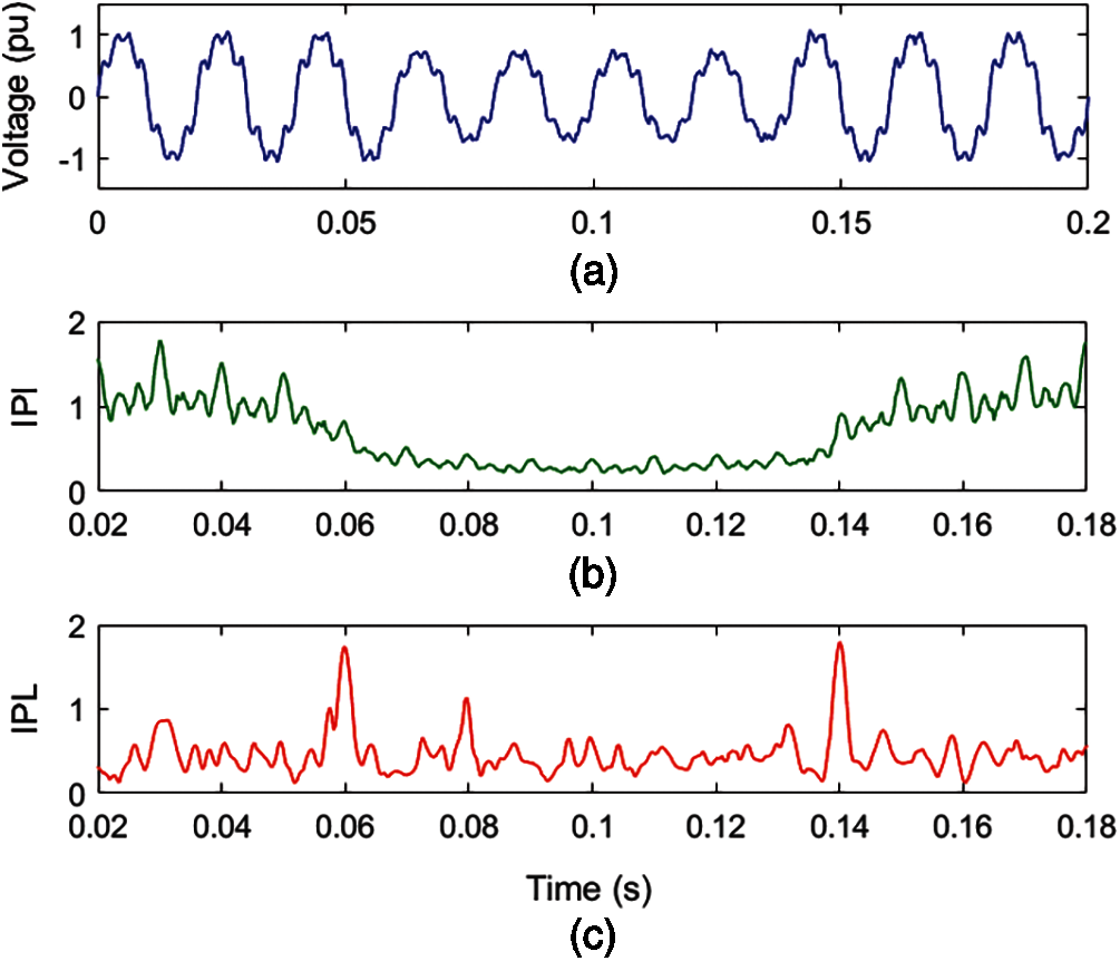
Figure 4: Voltage with sag and harmonics MPQ disturbance with superimposed noise of 20 dB SNR (a) Voltage (b) MPQ identification index (c) IPL

4.3 Voltage with MI and OT Multiple PQ Disturbance

The mathematical formulation is used to simulate a voltage with an associated MPQ disturbance of degree two multiplicity consisting of MI and OT, as shown in Fig. 5a. Voltage with MPQ disturbance is decomposed using the ST and HT to compute the MPQ identification index (IPI) and MPQ time location index (IPL). The IPI and IPL for MPQ disturbance of MI and OT are elaborated in Figs. 5b and 5c, respectively.

Fig. 5a details that voltage magnitude is reduced from 0.1 to 0.16 s and high magnitude ripples are available between 0.06 and 0.08 s. It is perceived from Fig. 5b that the magnitude of the IPI plot has reduced from 0.1 to 0.16 s to a very low magnitude, which indicates the incidence of a MI. Further, high-magnitude ripples are associated with the voltage signal between the time intervals of 0.06 and 0.08 s, indicating the presence of OT. It is perceived from Fig. 5c that there are high peaks at the time of 0.1 and 0.16 s which indicate the incidence and end of the MI disturbance. Further, high peaks at 0.06 and 0.08 s as well as high magnitudes between 0.06 and 0.08 s indicate the availability of OT associated with the voltage signal. Hence, plots of IPI and IPL indicate that there is a MPQ disturbance consisting of MI and OT associated with voltage. Further, the time of analysis of the MPQ disturbance consisting of MI and OT is small and equal to 0.161229 s.

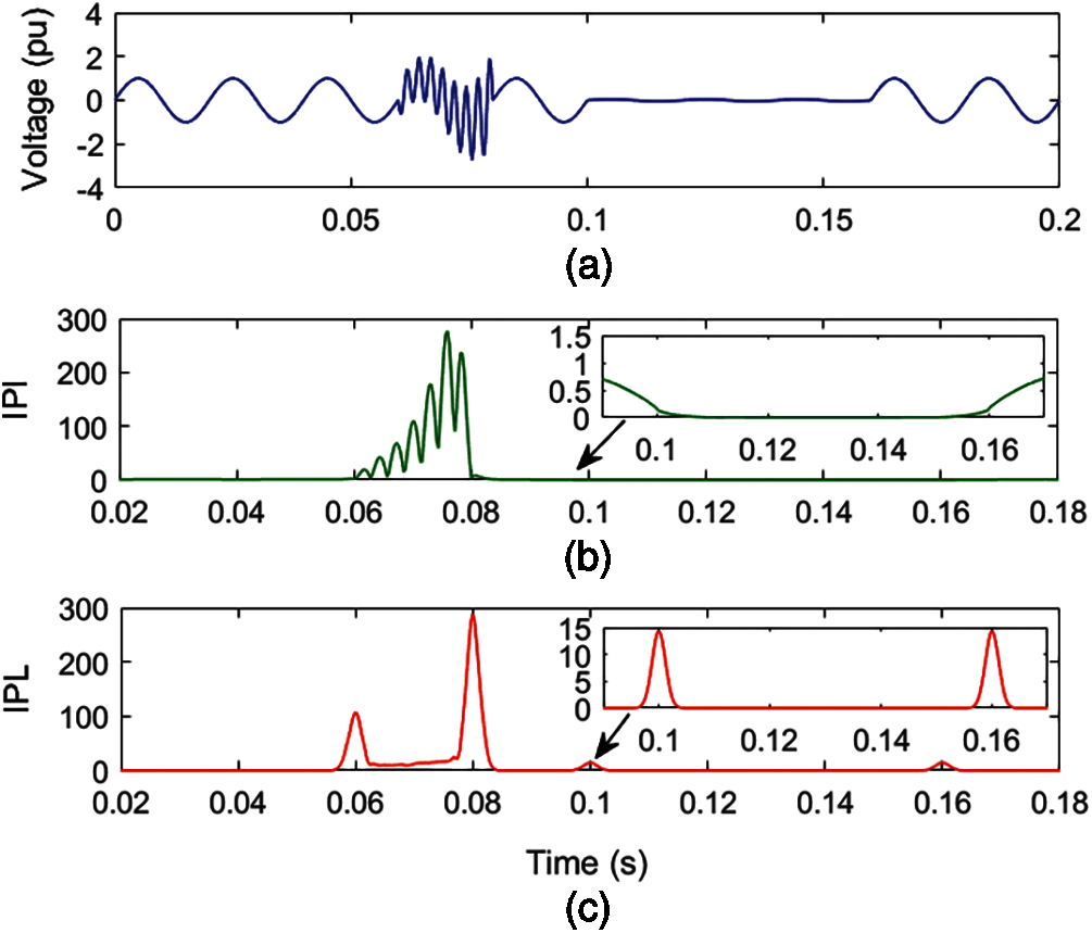
Figure 5: Voltage with momentary interruption and OT multiple PQ disturbance (a) Voltage (b) MPQ identification index (c) IPL

4.4 Voltage with Flicker and OT Multiple PQ Disturbance

In Fig. 6a, a voltage with an associated MPQ disturbance of degree two multiplicities, consisting of flicker and OT, is simulated using a mathematical formulation. Voltage with MPQ disturbance is decomposed using ST and HT to compute the MPQ identification index (IPI) and MPQ time location index (IPL). The IPI and IPL for MPQ disturbance of flicker and OT are elaborated in Figs. 6b and 6c in respective order.

Fig. 6a details that there are small variations in the magnitude of voltage over the complete time range. Further, high magnitude ripples are available between the 0.06 and 0.08 s. It is perceived from Fig. 6b that the magnitude of the IPI plot changes with a regular pattern, which indicates the availability of flicker. High magnitude along with ripples on the surface are associated with voltage between time intervals of 0.08 to 0.10 s, which indicates the presence of OT. It is perceived from Fig. 6c that the magnitude of the IPL plot changes with regular variations, which indicates the presence of flicker disturbance. Further, high peaks at 0.08 and 0.10 s as well as a high magnitude between 0.08 and 0.10 s are available, which indicates the presence of OT with voltage. Further, changes in the magnitude of the IPL plot during this time indicate the presence of flicker. Hence, plots of IPI and IPL indicate that there is an MPQ disturbance consisting of flicker and OT with voltage. Further, the time of analysis of the MPQ disturbance, comprised of flicker and OT, is small and equal to 0.061164 s.

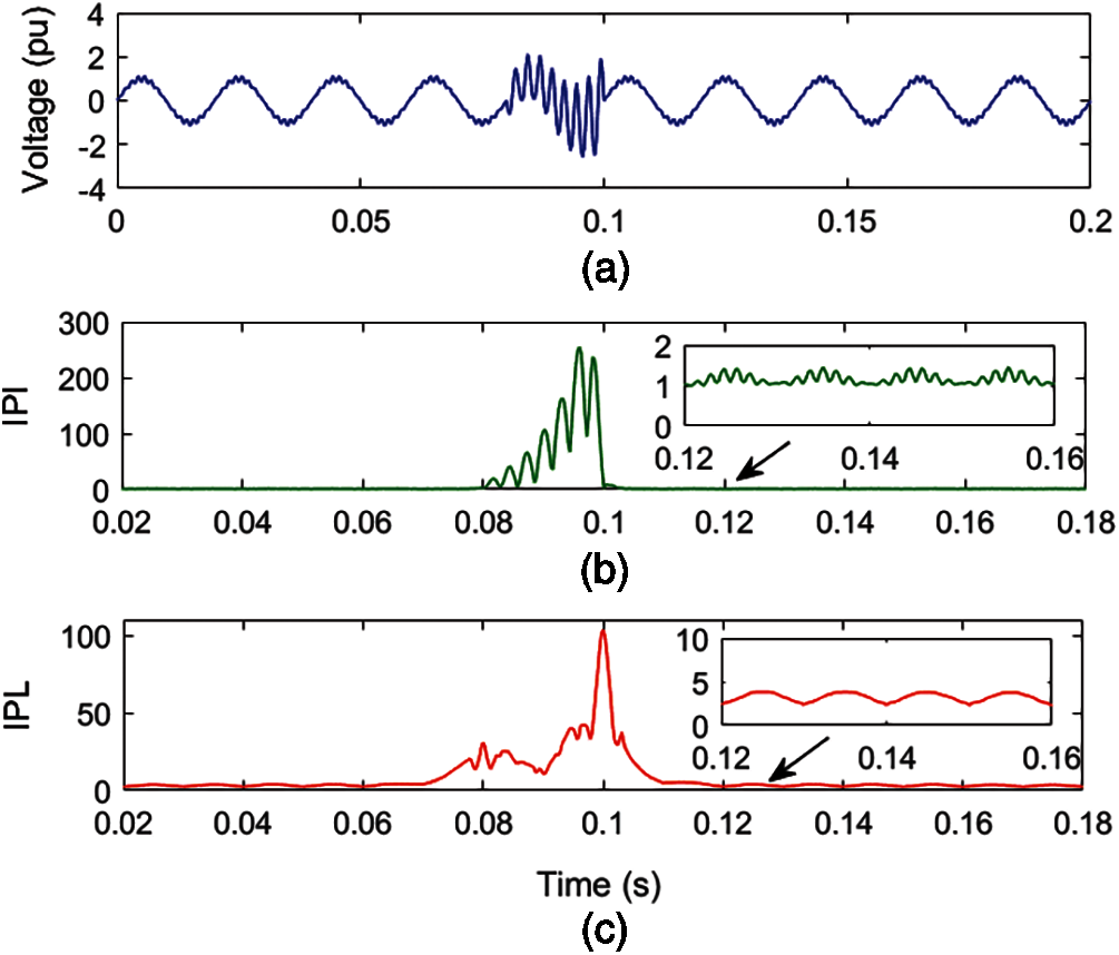
Figure 6: Voltage with flicker and OT multiple PQ disturbance (a) Voltage (b) MPQ identification index (c) IPL

4.5 Voltage with Sag and IT Multiple PQ Disturbance

A voltage signal with an associated MPQ disturbance of degree two multiplicities, consisting of sag and IT, is simulated using a mathematical formulation, as shown in Fig. 7a. Voltage with MPQ disturbance is decomposed by applying ST and HT to compute the MPQ identification index (IPI) and MPQ time location index (IPL). The IPI and IPL for MPQ disturbance of sag and IT are elaborated in Figs. 7b and 7c, respectively.

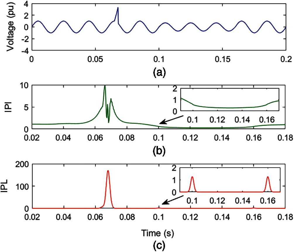
Figure 7: Voltage with sag and IT multiple PQ disturbance (a) Voltage (b) MPQ identification index (c) IPL

Fig. 7a details that voltage magnitude decreased to a low magnitude from 0.1 to 0.16 s and a high magnitude peak is available between 0.065 and 0.068 s. It is perceived from Fig. 7b that the value of the IPI plot has reduced to low values, from 0.1 to 0.16 s, which indicates the occurrence of sag disturbance. Further, high magnitude peaks are observed between 0.065 and 0.068 s which indicate the availability of IT. It is evaluated from Fig. 7c that there are high-magnitude peaks at instants of 0.1 and 0.16 s, which indicate the incidence and end of the sag disturbance. Further, a high-magnitude peak is observed between 0.065 and 0.068 s, which indicates the presence of IT. Hence, plots of IPI and IPL indicate that there is a MPQ disturbance consisting of sag and IT with voltage. Further, the time of analysis of the MPQ disturbance, comprised of sag and IT, is small and equal to 0.074325 s.

4.6 Voltage with Harmonics and IT Multiple PQ Disturbance

A voltage with an associated MPQ disturbance of degree two multiplicities, consisting of harmonics and IT, is simulated using a mathematical formulation, as shown in Fig. 8a. Voltage with MPQ disturbance is decomposed using ST and HT to compute the MPQ identification index (IPI) and MPQ time location index (IPL). The IPI and IPL for MPQ disturbance of harmonics and IT are elaborated in Figs. 8b and 8c sequentially.

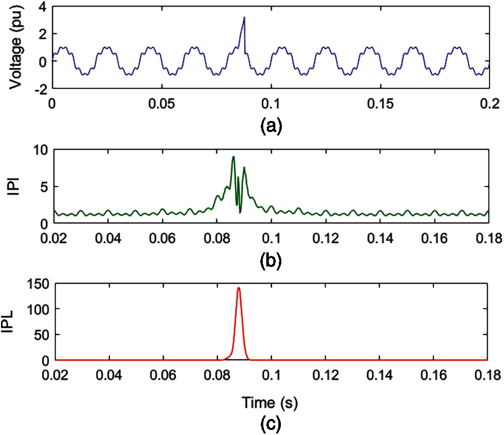
Figure 8: Voltage with harmonics and IT Multiple PQ disturbance (a) Voltage (b) MPQ identification index (c) IPL

Fig. 8a details that a high-magnitude peak is available between 0.085 and 0.088 s and ripples are superimposed over voltage. It is perceived from Fig. 8b that high magnitude peaks are observed between 0.065 and 0.068 s which indicate the presence of IT. Further, low-magnitude ripples are associated over the entire time range, which indicates the presence of harmonic components. It is evaluated from Fig. 8c that there is a high value peak from 0.085 to 0.088 s which indicates the presence of IT. Hence, plots of IPI and IPL indicate that there is a MPQ disturbance consisting of IT and harmonics pertaining to voltage. Further, the time of analysis of the MPQ disturbance, comprised of sag and harmonics, is small and equal to 0.163903 s.

4.7 Voltage with Sag and Notch Multiple PQ Disturbance

A voltage with an associated MPQ disturbance of degree two multiplicities, consisting of sag and notch, is simulated and elaborated in Fig. 9a. Voltage with MPQ disturbance is decomposed using ST and HT to compute the MPQ identification index (IPI) and MPQ time location index (IPL). The IPI and IPL for MPQ disturbance of harmonics and IT are elaborated in Figs. 9b and 9c, respectively.

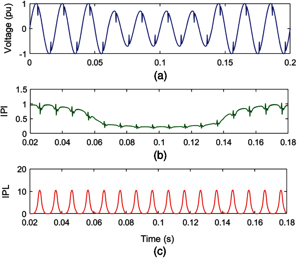
Figure 9: Voltage with sag and notch multiple PQ disturbance (a) Voltage (b) MPQ identification index (c) IPL

Fig. 9a details that voltage magnitude decreased to low values from 0.06 to 0.14 s and relatively low-magnitude ditches are observed at regular intervals. It is perceived from Fig. 9b that the magnitude of the IPI plot has decreased to low values, from 0.06 to 0.14 s, which indicates the incidence of sag disturbance. Further, a pattern of two spikes where one spike has a high magnitude and one spike has a low magnitude is observed at regular intervals, indicating the availability of notches. It is evaluated from Fig. 9c that there are high-magnitude peaks at regular intervals which indicate the occurrence of notches. Hence, plots of IPI and IPL indicate that there is an MPQ disturbance consisting of sag and notches pertaining to the voltage signal. Further, the time of analysis of the MPQ disturbance, comprised of sag and notches, is small and equal to 0.080542 s.

4.8 Voltage with Sag, Harmonics and OT Multiple PQ Disturbance

In Fig. 10a, a voltage is simulated with a three-degree multiplicity MPQ disturbance consisting of sag, harmonics, and OT using a mathematical formulation. Voltage with MPQ disturbance is decomposed using ST and HT to compute the MPQ identification index (IPI) and MPQ time location index (IPL). The IPI and IPL for MPQ disturbance of sag, harmonics and OT are elaborated in Figs. 10b and 10c sequentially.

Fig. 10a details that the voltage magnitude decreases from 0.1 to 0.16 s and ripples are superimposed over the voltage. Further, transient ripples of high magnitude are available between the time intervals of 0.06 to 0.08 s. It is perceived from Fig. 10b that the magnitude of the IPI plot has reduced from 0.1 to 0.16 s, which indicates the incidence of the voltage sag. Further, low-magnitude ripples are associated over the complete time range, which indicates the availability of the harmonic components. A very high magnitude of IPI index with transient ripples on the top surface is observed between time intervals of 0.06 to 0.08 s, indicating the availability of the OT. It is observed from Fig. 10c that there are high-magnitude peaks at the times of 0.10 and 0.16 s, which indicate the incidence and end of the sag disturbance. Further, high peaks at 0.06 and 0.08 s as well as high magnitudes between 0.06 and 0.08 s are available, which indicate the presence of OT associated with the voltage signal with MPQ disturbance. Hence, plots of IPI and IPL indicate that there is a MPQ disturbance consisting of sag, harmonics and OT associated with the voltage. Furthermore, the computational time for analyzing the MPQ disturbance, which includes sag and harmonics, is small, equaling 0.070415 s.

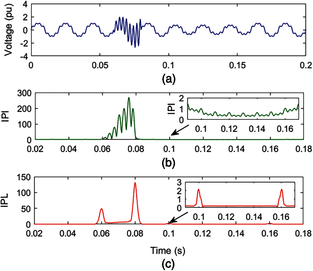
Figure 10: Voltage with sag, harmonics and OT multiple PQ disturbance (a) Voltage (b) MPQ identification index (c) IPL

4.9 Voltage with Flicker, Harmonics and IT Multiple PQ Disturbance

A voltage signal with a three-degree multiplicity MPQ disturbance consisting of flicker, harmonics, and IT is simulated using a mathematical formulation and illustrated in Fig. 11a. Voltage with MPQ disturbance is reduced using ST and HT to compute the MPQ identification index (IPI) and MPQ time location index (IPL). The IPI and IPL for MPQ disturbance of flicker, harmonics and IT are elaborated in Figs. 11b and 11c sequentially.

Fig. 11a details that a high-magnitude peak is available between 0.085 and 0.088 s, and ripples are superimposed over the voltage signal. Ripples of low magnitude on the crest and trough of the waveform indicate the presence of flicker. It is perceived from Fig. 11b that high peaks are seen between 0.085 and 0.088 s, which indicate the presence of IT. Three peaks are available on the surface of high magnitude between 0.085 and 0.088 s are due to the presence of harmonics. A pattern of three peaks over the entire time range indicates the availability of harmonics, where low-magnitude ripples on the surface of these peaks indicate the presence of flicker. Hence, low magnitude variations along with ripples associated over the complete time range of the voltage signal indicate the availability of harmonic components and flicker. It is evaluated from Fig. 11c that there is a high peak between 0.085 and 0.088 s which indicates the presence of IT. Furthermore, variations of low magnitude on the surface of the IPL plot indicate the presence of flicker. Hence, plots of IPI and IPL indicate that there is a MPQ disturbance consisting of flicker, IT and harmonics pertaining to voltage. Further, the time of analysis of the MPQ disturbance consisting of flicker, IT, and harmonics is small and equal to 0.084994 s.

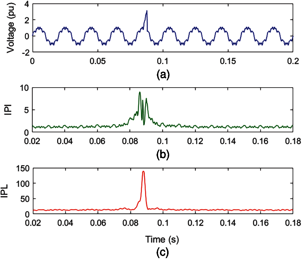
Figure 11: Voltage with flicker, harmonics and IT multiple PQ disturbance (a) Voltage (b) MPQ identification index (c) IPL

4.10 Classification of Multiple PQ Disturbances

The MPF1, MPF2, MPF3, and MPF4 features are computed using the mathematical relations described in Section 3.5 and shown in Table 3. Different values of these features are utilized for classification of MPQ disturbances using decision rules. The MPQ classification tree and decision rules are described in Fig. 12.

The classification of MPQ disturbances started using the feature MPF1 and was grouped into two groups. If MPF1 > 100, then disturbances are included in Group-GA else grouped in Group-GB. Disturbances of Group-GA are categorized in two groups using the feature MPF3. If MPF3 > 500, then disturbances are included in Group-GA1, which are MPD2, MPD3, and MPD7. If MPF3 > 500, then disturbances are included in Group-GA2, which are MPD4, MPD5, and MPD8. The disturbances MPD0, MPD1 and MPD6 are grouped in Group-GB. Disturbances of Group-GB, Group-GA1 and Group-GA2 are categorized one by one using the decision rules described in Fig. 12. The end nodes of the decision tree described in Fig. 12 contain the MPQ disturbances. All the investigated MPQ disturbances have been categorized effectively using the decision rules.

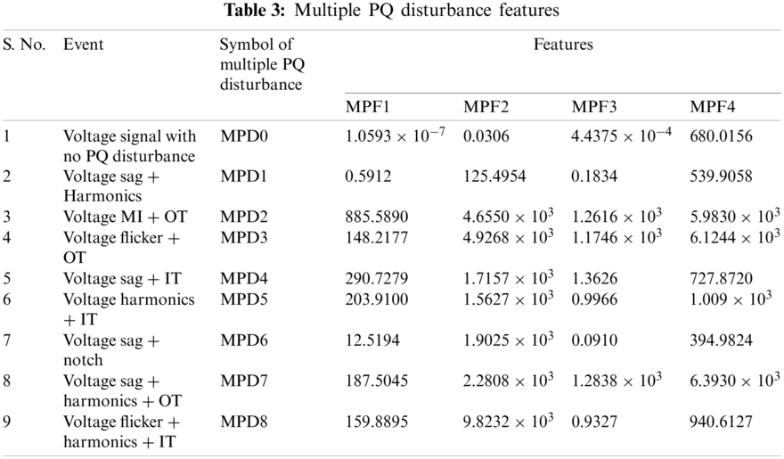
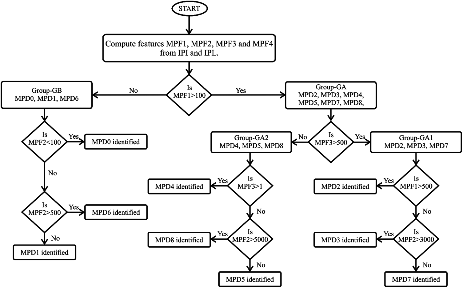
Figure 12: MPQ classification tree

5  Performance of Algorithm

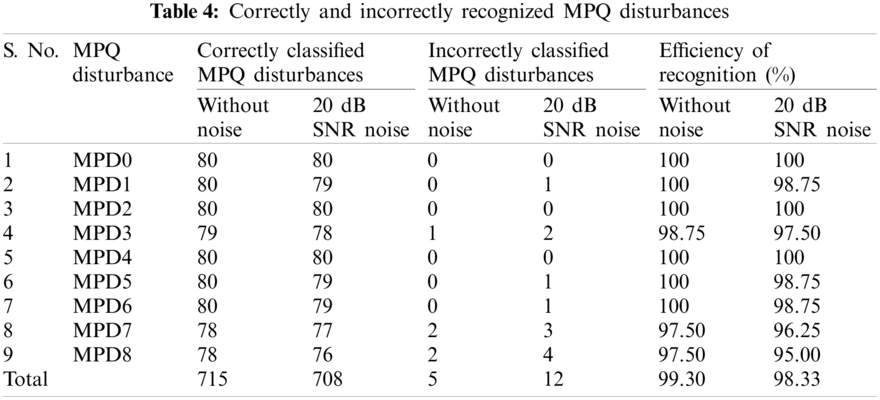
The performance of the hybrid parallel algorithm and decision rules-based approach is evaluated for identification and classification of the 80 disturbances for every MPQ event. This set of data is computed by varying parameters such as amplitude, frequency, noise levels, etc. The performance is measured in both noise-free and noisy environments. A list of accurately and inaccurately identified and classified MPQ disturbances is included in Table 4. It is perceived that the algorithms identify and classify the MPQ disturbances with accuracy higher than 99% in the noise-free environment. It effectively recognizes the MPQ disturbances with accuracy higher than 98% in the noisy environment with 20 dB SNR.

The performance of the RBDT based classifier driven by the features computed from the IPI and IPL indices is also evaluated using the indices such as root mean square error (RMSE), mean absolute error (MAE), precision, and recall. RMSE is a principal metric which effectively measures the difference between the values predicted by the classifier and their true value, as defined by the below relation [25]:

RMSE=1M∑i=1M(Pc(i)−Tc(i))2 (28)

where Pc(i): probability of prediction of instance i belonging to class c, Tc(i): actual probability, M: total number of positive samples (P) and negative samples (N). MAE alternatively represents the RMSE. It averages the magnitude of the individual errors without considering the signs as detailed below [25]:

MAE=1M∑i=1M|Pc(i)−Tc(i)| (29)

Precision indicates the capability of the classifier for determining the positive labels using one vs. all approach and defined as detailed below [26]:

Precision=1M∑i=1MTPiTPi+FPi (30)

where TPi: true positive, FPi: false positive. Recall indicates the average value per-class effectiveness of a classifier for identification of class labels and defined as detailed below [26]:

Recall=1M∑i=1MTPiTPi+FNi (31)

where FNi: false negative.

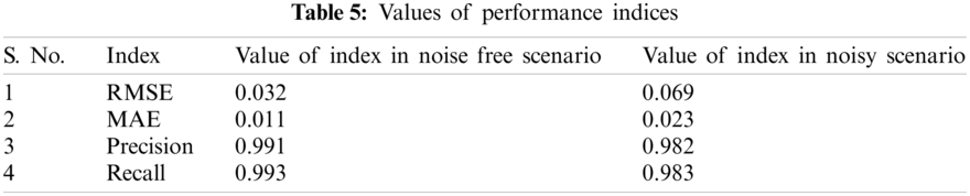
The performance of the RBDT based classifier driven by the features computed using ST and HT is evaluated in terms of RMSE, MAE, precision and recall. This is achieved using the 80 data sets of every MPQ disturbance used by the user. Table 5 summarizes the knowledge modeling concept and values computed for these data sets in the noise-free and noisy scenarios. It is observed that RMSE and MAE have minimum values in the noise free condition and these values are relatively high during the noisy condition. Further, the precision and recall have high values that approach unity. The performance indices RMSE, MAE, precision and recall indicate that the proposed algorithm using ST and HT with RBDT effectively recognizes the MPQ disturbance.

5.1 Performance Comparison

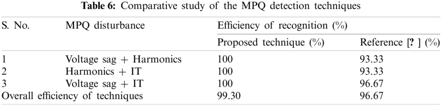
The efficacy of the results of the study introduced in this manuscript is compared with the technique using the ST and RBDT and reported in [27]. The ST and RBDT-based MPQ identification technique recognizes the MPQ disturbances with an accuracy of 96.67%. However, the technique designed in this manuscript using the parallel algorithm supported by ST & HT and decision rules identifies the MPQ disturbances with an accuracy higher than 99% in the noise free environment and with an accuracy higher than 98% in the noisy environment with 20 dB SNR. The performance of the proposed ST and HT with RBDT based method is compared with the technique reported in [27] for the three MPQ disturbances in the noise-free environment and provided in Table 6. It is observed that the proposed technique using ST and HT with RBDT is more effective compared to the ST and RBDT based technique reported in [27]. Hence, it is established that the technique investigated in this manuscript is superior compared to the ST and RBDT techniques available in [27].

6  Application of Proposed Algorithm to Recognize MPQ Disturbances Associated to Real-Time Power System Network

The proposed ST and HT with RBDT based algorithm for recognition of MPQ disturbances has been tested to identify the MPQ disturbances associated with the line-to-ground (LG) fault event incident on the practical power system network of Rajasthan State of India. Details of the real-time transmission network, such as generations, number of grid sub-stations (GSS), circuit length of the transmission lines of all voltages, and loads used for the study are available in [28]. Transmission and distribution lines are operated on the voltage levels of 765, 400, 220, 132, 33, 11 and 0.44 kV. The nature of the generating machines integrated into this network includes nuclear power plants (NPP), thermal power plants (TPP), wind power plants (WPP), solar power plants (SPP) and biomass power plants (BPP). Voltage data of an auto-recloser installed on a power line during a scenario of a line-to-ground (LG) fault incident on the R-phase is taken from the disturbance recorder. This signal is processed using the proposed ST and HT with RBDT based algorithm and IPI and IPL plots are computed. Fig. 13 depicts the IPI and IPL plots during the LG fault scenario. According to Fig. 13a, the LG fault event occurs on the fourth cycle and is cleared on the ninth cycle. Fig. 13b demonstrates that the MI disturbances are available between the 4th cycle and the 9th cycle due to the incidence of the LG fault. Further, a high magnitude peak at the time of the 9th cycle indicates the presence of an IT disturbance. Ripples from the 4th cycle indicate the presence of transients during the fault period and post-fault period. Fig. 13c demonstrates that high-magnitude peaks at the time of the 4th cycle and 9th cycle locate the MI disturbance in the time range, while continuous ripples from the 4th cycle indicate the presence of transient components available during the fault period and post-fault period.

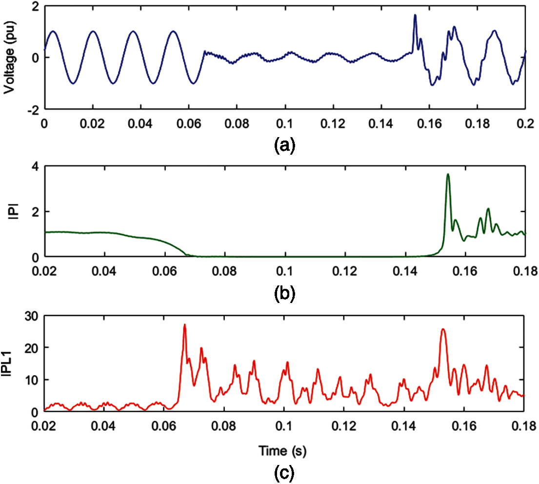
Figure 13: MPQ disturbances due to LG fault on a practical distribution network (a) Voltage (b) MPQ identification index (c) IPL

7  Conclusion

This paper designed a robust technique to identify and classify MPQ disturbances. This is achieved using the ST, HT and decision rules. The IPI and IPL indices are used to identify and locate the MPQ disturbances. These MPQ disturbances have been classified in different categories using the decision rules. It is concluded that IPI has different patterns for various types of MPQ disturbances which effectively identify all the MPQ disturbances. Further, the proposed IPL effectively identifies the initiation and end of the MPQ disturbances and thereby effectively locates the MPQ events. All the investigated MPQ events have been effectively classified using the decision rules in both the noise-free and noisy environments with a 20 dB SNR with accuracy higher than 98%. This is achieved in a time period less than 0.3 s. Further, the effectiveness of the proposed RBDT classifier is also established using indices such as RMSE, MAE, precision, and recall. The performance of the technique is found to be superior compared to the ST and RBDT techniques in terms of classification accuracy of MPQ disturbances and reduced computational time. The proposed algorithm effectively identified MPQ disturbance incidents on the real-time power system network.

Funding Statement: The authors received no specific funding for this study.

Conflicts of Interest: The authors declare that they have no conflicts of interest to report regarding the present study.

This work is licensed under a Creative Commons Attribution 4.0 International License, which permits unrestricted use, distribution, and reproduction in any medium, provided the original work is properly cited.