| Energy Engineering |
DOI: 10.32604/ee.2022.018241
ARTICLE
Performance Evaluation of Small-channel Pulsating Heat Pipe Based on Dimensional Analysis and ANN Model
1Fluids and Thermal Engineering Research Group, Faculty of Engineering, University of Nottingham, Nottingham, NG7 2RD, UK
2Ningbo Tech University, Ningbo, 315100, China
3Research Centre for Fluids and Thermal Engineering, University of Nottingham Ningbo China, Ningbo, 315100, China
*Corresponding Author: Neng Gao. Email: gao@zju.edu.cn
Received: 09 July 2021; Accepted: 10 September 2021
Abstract: The pulsating heat pipe is a very promising heat dissipation device to address the challenge of higher heat-flux electronic chips, as it is characterised by excellent heat transfer ability and flexibility for miniaturisation. To boost the application of PHP, reliable heat transfer performance evaluation models are especially important. In this paper, a heat transfer correlation was firstly proposed for closed PHP with various working fluids (water, ethanol, methanol, R123, acetone) based on collected experimental data. Dimensional analysis was used to group the parameters. It was shown that the average absolute deviation (AAD) and correlation coefficient (r) of the correlation were 40.67% and 0.7556, respectively. For 95% of the data, the prediction of thermal resistance and the temperature difference between evaporation and condensation section fell within 1.13 K/W and 40.76 K, respectively. Meanwhile, an artificial neural network model was also proposed. The ANN model showed a better prediction accuracy with a mean square error (MSE) and correlation coefficient (r) of 7.88e-7 and 0.9821, respectively.
Keywords: Pulsating heat pipe; oscillation; heat transfer; correlation; ANN model
Nomenclature
| b, b | bias |
| Cv | covariance |
| cp | specific heat (J/(kg∙K)) |
| di | inner diameter (m) |
| g | gravity (m/s2) |
| l | length (m) |
| N | number of turns |
| Q | Power (W) |
| q | heat flux (W/m2) |
| R | thermal resistance (K/W) |
| r | correlation coefficient |
| ΔT | temperature difference (K) |
| T | temperature (K) |
| x, x | input |
| y, y | output |
| Y | data value |
| Greek Symbols | |
| λ | thermal conductivity (W/(m∙K)) |
| μ | dynamic viscosity (Pa∙s) |
| πi | dimensionless number |
| ρl | liquid density (kg/m3) |
| σ | surface tension (N/m) |
| φ | filling ratio |
| ω, ω | weight |
| Subscript | |
| e | evaporation section |
| exp | experiment |
| pre | predicted results |
With the rapid development of the electronics industry, chips are becoming increasingly compact, generating a larger amount of heat in an ever-smaller physical size. This additional heat must be efficiently dissipated by the thermal network. Otherwise, the chips will suffer significantly from lower efficiency, short life-span, and even physical damage [1]. Thermal management of chips has and will continue to become one of the most essential technologies. Against this context, pulsating heat pipes, or oscillating heat pipes, characterised by excellent heat transfer ability, simple physical structure, and high flexibility for miniaturisation, are believed to be one of the most promising prospective technologies to meet the requirement of higher heat flux dissipation [2,3]. The PHP consists of connected serpentine channels, and is divided into evaporation, adiabatic, and condensation sections [4]. Considering the small diameter of PHP channel, the influence of the working fluid’s surface tension is very important [5]. A train of liquid slugs and vapor plugs are formed within the channel, and through their oscillation motions, the heat is dissipated [6]. Many studies were conducted to study its heat transfer characteristics by theoretical modelling and experimental investigation over the past decades [7–9]. Some potential applications of PHP in electronics cooling, heat exchangers, and solar energy utilisation also have been preliminarily investigated [10].
Reliable prediction of the performance of PHP has been a hot research topic as it plays an essential role to promote its application. Generally, there are two basic methods to predict performance of the PHP, classic heat transfer correlations and ANN network models. For classic heat transfer correlations, typical heat transfer dimensionless numbers, like the Kutateladze number, Morton number, Jackob number, Bond number, and Prandtl number, are correlated to study the influence of various geometric, property and operating parameters. In 2003, Khandekar et al. [11] presented a correlation for PHP by theoretical analysis of several basic heat and mass transfer mechanisms in the PHP. The accuracy of the correlation was within ±30%. After that, Katpradit et al. [12] presented two correlations for the performance of PHP in vertical and horizontal heated models. The standard deviations of these were ±18% and ±29%, respectively. Qu et al. [13] introduced the influence of Bond number and Morton number, revealing another correlation for vertical PHPs. It was suggested that the deviation of the correlation was ±40%, comparing with the collected experimental data. Kholi et al. [14] proposed another new heat transfer correlation. The influence of the filling ratio was separately considered by a polynomial. The correlation successfully coincided with the performance of PHPs with ±30% accuracy. Another remarkable method to predict the performance of the PHP is by the ANN models, as ANN models have apparent advantages in analysing non-linear systems and have been extensively used in pattern recognition, property parameter prediction, and heat transfer regression [15,16]. E et al. [17] presented an ANN model using the filling ratio, heat flux, and inclination angle of the PHP as the input. The relative average error between the experimental data and predicted results was 4% as claimed, showing good accuracy of the ANN models. Ali et al. [18] built another ANN model also with filling ratio, heat flux, and inclination angle as the input parameters. It was shown that the relative errors of 90% of the data points were less than 5%, and the remaining points lay between 5% and 12%. Another ANN model was suggested by Patel et al. [19], with inner diameter, outside diameter, lengths of evaporation and condensation section, number of turns, heating power, filling ratio, and inclination angle as the inputs. The working fluids were examined by index. The mean absolute relative deviations fell within 24.12% for 68% of the data. A more general method was proposed by Wang et al. [20] using Kutateladez number, Morton number, Bond number, Prandtl number, Jackob number, the ratio of evaporation length and inner diameter, and the number of turns as selected input parameters for PHP with various working fluids. The correlation coefficient of the proposed ANN model was 0.9824, showing a very high agreement.
The existing heat transfer correlations and ANN models provide remarkable solutions to estimate the performance of the PHP. However, the proposed heat transfer correlations were commonly regressed from the specific range of the experimental data, and with relative low accuracy. More effort is still required to improve the accuracy of these models, and further validate the suitable application range. Despite the excellent accuracies of the ANN models, their application is highly dependent on the collected data and with certain parameters as the input. In this paper, the impact of typical geometrical parameters, properties of working fluids, and operating parameters were considered by dimensional analysis first to obtain the dimensionless numbers. A heat transfer correlation was proposed based on these dimensionless numbers. Following that, an ANN model was also presented to correlate the thermal resistance of PHP, taking advantage of its high accuracy.
For performance prediction, the most important factor is to figure out the relation between the heat flux and the related geometrical, property, and operating parameters,
To analyse the impact of various parameters on the performance of PHP, the dimensional analysis was used to get the dimensionless parameters. This method is conducted to group the influence of different parameters and generalise various operational conditions. The impacts of geometric, property, and operating parameters were considered. The correlation was presented as,
The dimensions of R, ρl, λ, μ, σ, cp, di, le, q, g are θM-1L-2T3, ML-3, MLT-3θ-1,ML2=-1T-1, MT-2L, L2T-2θ-1, L, L, MT-3, LT-2, respectively. There are ten parameters, and four basic dimensions in Eq. (1). Therefore, we can get six dimensionless parameters according to Buckingham π theorem. If select ρl, λ, μ, d as the basic parameters, the six dimensionless parameters are defined by,
Thus, we get the correlation
It is well-known that the physical properties change with temperature, and a reference temperature is needed to calculate them. To evaluate the thermal-physical properties in the Eqs. (2)–(8), the coolant temperature was selected as the reference temperature rather than the average of evaporation and condensation section temperature, as it is the only known temperature in the design stage. The temperatures of the evaporation and condensation section can be further obtained based on the thermal resistance and heat transfer correlations [20].
2.2 Experimental Data Collected
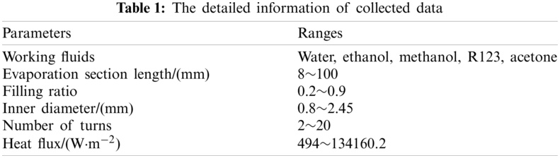
To obtain the performance prediction models, the experimental data for the bottom-heated PHP with various inner diameters, filling ratios, turn numbers, evaporation lengths, and working fluids were gathered from the literature [21–43]. The parameters’ information of the collected data was presented in Table 1. The ranges of these parameters cover wide operating conditions.
3 Heat Transfer Correlation for PHP
Based on the experimental data and dimensional analysis presented above, the following heat transfer correlation was obtained to predict the performance of PHP based on least square method.
The prediction performance of the heat transfer correlation is shown in Fig. 1. The MSE and the correlation coefficient between the experimental data and correlation were 9.12e-6 and 0.755, respectively. The average absolute deviation (AAD) of the prediction was 47.65%. While the prediction for most experimental data fell within Region A with deviation within ±50%, there were some data beyond this range and lower than –50%, as indicated by Region B.
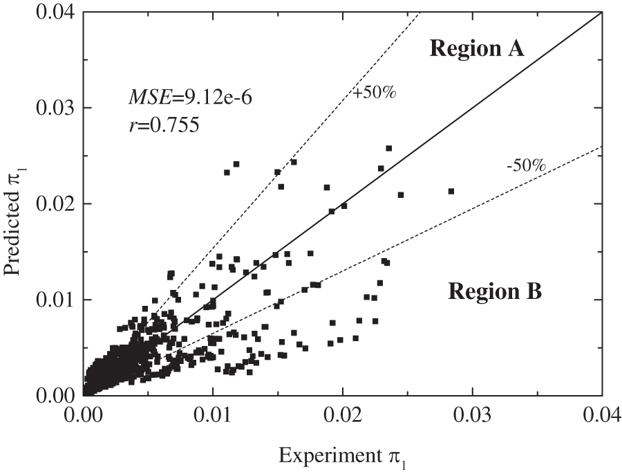
Figure 1: The prediction of heat transfer correlation
It is noteworthy to further analyse the prediction characteristics of the correlation (10), by revealing the reasons of great deviation in Region B. When evaluating the heat transfer performance of the PHP, the thermal resistance and temperature difference between the evaporation and condensation section are very important indicators. Therefore, their prediction deviations are used in this paper to show the performance of proposed correlation, and they are given by,
The influence of thermal resistance on the prediction of ΔR and Δ (Te-Tc) was shown in Fig. 2. As can be seen from Fig. 2a, the prediction deviation of thermal resistance generally increased with the thermal resistance. The ΔR of 95% data was within 1.13 K/W. While the prediction was good for lower thermal resistance, the prediction saw quite great deviations when the thermal resistance was greater than 2 K/W. Nearly all the great deviations occur in this range. Meanwhile, the prediction of ΔR was also influenced by the working fluids. The average deviation of ΔR for water, R123, ethanol, acetone, and methanol were –0.14 K/W, 0.49 K/W, –0.007 K/W, 0.058 K/W and 0.025 K/W, respectively. When it comes to the prediction of Δ (Te-Tc), as indicated in Fig. 2b. For 95% of the total data, the deviations of Δ (Te-Tc) were within 40.76 K, and the great deviation also occurs for the higher thermal resistance. The average of Δ (Te-Tc) for water, R123, ethanol, acetone, and methanol were –6.147, 24.39, –2.51, 2.1, and 0.74 K, respectively. The influence of the heat flux is presented in Fig. 3. The prediction accuracies of ΔR and Δ (Te-Tc) were generally poor when the heat flux was lower than 40,000 W/m2.
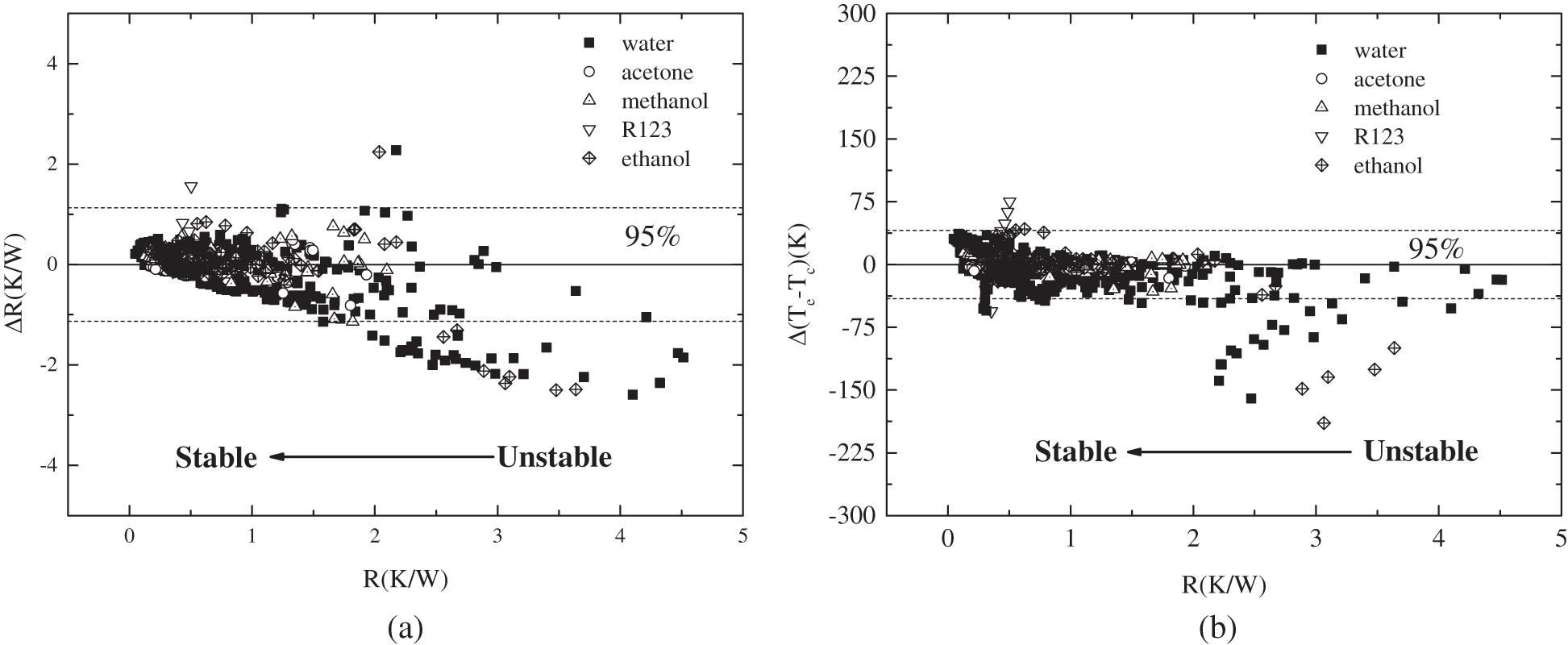
Figure 2: The influence of thermal resistance on prediction of (a) ΔR; (b) Δ (Te-Tc)
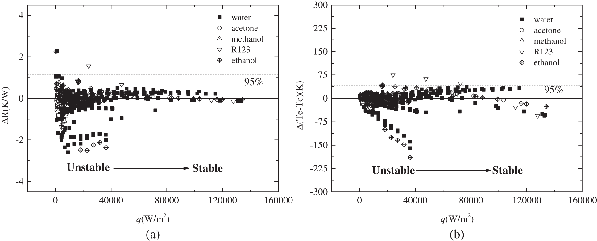
Figure 3: The influence of heat flux on prediction of (a) ΔR; (b) Δ (Te-Tc)
A possible reason which may contribute to the great deviations of the correlation for higher thermal resistance and lower heat flux is when the heat flux is in a lower level, the PHP experiences a condition of pre-startup or quasi-startup, in which status the operating of PHP is not stable, and is characterised by different flow patterns compared to the stable oscillation at a higher heat flux level [44]. As a result, the experimental data scatter is great between different studies. It is therefore very difficult to correlate an accurate heat transfer correlation for various studies. Meanwhile, the thermal resistance of PHP is usually very large when the heat flux is at a lower level. Therefore, the deviations are generally great for lower heat flux and larger thermal resistance cases. Further investigation on different operating patterns of PHP and the proposed correlation separately is expected to benefit the accuracy improvement.
A new, fully connected ANN model was defined to correlate the performance of PHP, to take advantage of excellent it accuracy in non-linear analysis. The collected experimental data were divided into training, validation, and testing data sets randomly at the ratio of 70%, 15%, and 15% respectively. To avoid too complex an ANN model, only one hidden layer was used. The parameters considered in above section were used as the input of ANN model. In an ANN model, the outputs of each node in l-th layer are the function of weights and bias, and are given by,
Therefore, the output of the ANN model was presented by,
For all input data, the following function was used to pre-processes the input data,
The transfer function is used to pre-process the data. The following sigmoid function was used,
The error of the ANN model can be evaluated by,
The linear function was implemented for the output layer. Due to great stability, flexibility, and adaptability of Levenberg- Marquardt algorithm, it was selected as the learning algorithm of the ANN model. The prediction performance of the ANN model is usually described by correlation efficient (r) and mean square error (MSE), and they are defined by the following equations [45]:
A trial-and-error method was implemented to find the optimal hidden layer neuron number. The analysis result is shown in Fig. 4. It was shown that the MSE changed with neuron numbers, and with the increase of the number, the MSE generally decreased. To balance the accuracy and complexity, the optimal hidden layer neuron number was set at 12. The MSE of training, validation, testing and, total data set were 8.59e-7, 5.69e-7, 6.71e-7, and 7.88e-7, respectively. The structure of the proposed ANN model was illustrated in Fig. 5.
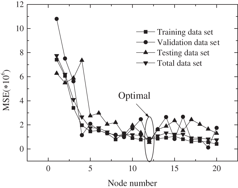
Figure 4: The change of MSE with hidden layer neural number
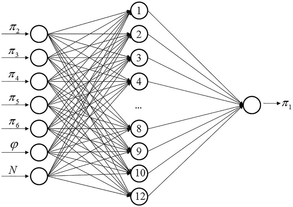
Figure 5: The structure of the presented ANN model
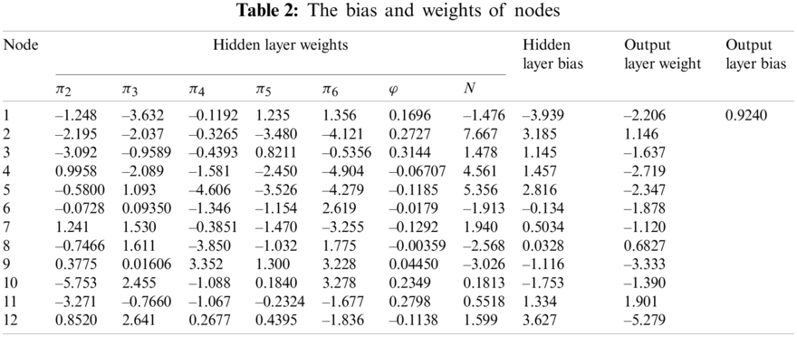
The predictions for the training, validation, testing, and total data set are further shown in Fig. 6. As can be seen, when the hidden layer was with 12 neurons, the prediction of the proposed ANN model coincided well with the experimental data. The MSE and correlation coefficient were 7.88e-7 and 0.9821, respectively. The optimised bias and weights are presented in Table 2.
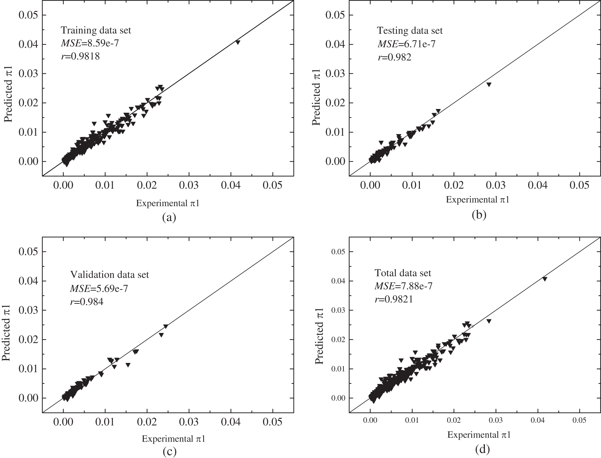
Figure 6: The performance of the data sets (a) training (b) testing (c) validation (d) total
The influence of thermal resistance on the prediction of ΔR and Δ (Te-Tc) is presented in Fig. 7. As can be seen, the prediction of ΔR was better with lower thermal resistance. For ΔR prediction, more than 95% of experimental data fell within ±0.39 K/W, which showed an excellent accuracy of the ANN model. The prediction was also influenced by working fluids. For water, acetone, methanol, R123, and ethanol, the average ΔR were 0.0036, 0.095, –0.015, –0.083, and 0.006 K/W, respectively. Regarding the prediction of Δ (Te-Tc), 95% of data fell within ±19 K. Meanwhile, the average of Δ (Te-Tc) for water, acetone, methanol, R123, and ethanol were 1.18, 1.98, –1.04, –9.67, and 0.18 K, respectively. The influence of heat flux is shown in Fig. 8. With increasing heat flux, the prediction of ΔR became more accurate, while the prediction of Δ (Te-Tc) did not show any relevance to the heat flux.
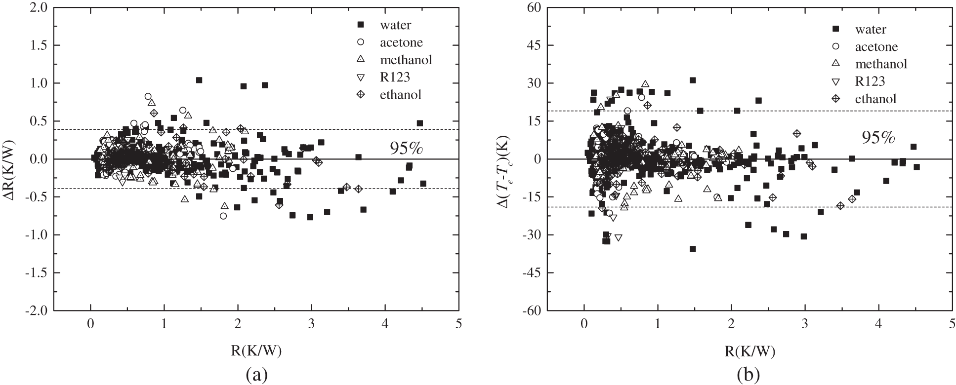
Figure 7: The influence of thermal resistance on prediction of (a) ΔR; (b) Δ (Te-Tc)

Figure 8: The influence of heat flux on prediction of (a) ΔR; (b) Δ (Te-Tc)
In this paper, the dimensional analysis was conducted to group various influence parameters to predict the heat transfer performance of PHP with various working fluids (water, ethanol, methanol, R123, acetone). A heat transfer correlation was firstly presented based on the collected data. The coefficient correlation and AAD of the correlation were 0.755 and 47.65%, respectively. Further analysis suggested that most great deviation occurred for higher thermal resistance (>2 K/W) or lower heat flux (<40000 W/m2). For 95% of the data, the prediction of thermal resistance and temperature difference between evaporation and condensation section were 1.13 K/W and 40.76 K, respectively. In addition, an ANN model was also proposed to better predict the performance of PHP, considering its great advantage in solving and correlating complex non-linear problems. The proposed ANN model has 7 nodes, 12 nodes, and 1 node in input layer, hidden layer, and output layer, respectively. It was found that the prediction agreed with the experimental data very well, with the MSE and R at 7.88e-7 and 0.9821, respectively. Furthermore, the ANN model also showed good accuracy in predicting the ΔR and Δ (Te-Tc).
Despite that, further studies regarding the internal heat transfer characteristics and oscillation flow patterns of the PHP in various conditions still need to be conducted. Revealing them will help to build more accurate models and boost the application of PHP.
Funding Statement: This work is funded by National Natural Science Foundation of China (No. 51906216).
Conflicts of Interest: The authors declare that they have no conflicts of interest to report regarding the present study.
1. Fan, S., Duan, F. (2020). A review of two-phase submerged boiling in thermal management of electronic cooling. International Journal of Heat and Mass Transfer, 150(41501), 119324. DOI 10.1016/j.ijheatmasstransfer.2020.119324. [Google Scholar] [CrossRef]
2. Han, X., Wang, X., Zheng, H. (2016). Review of the development of pulsating heat pipe for heat dissipation. Renewable and Sustainable Energy Reviews, 59(3), 692–709. DOI 10.1016/j.rser.2015.12.350. [Google Scholar] [CrossRef]
3. Chao, H., Wang, X., Gao, X. (2017). Experimental research on the start-up characteristics and heat transfer performance of pulsating heat pipes with rectangular channels. Applied Thermal Engineering, 126, 1058–1062. DOI 10.1016/j.applthermaleng.2017.02.106. [Google Scholar] [CrossRef]
4. Wang, X., Zheng, H., Si, M. (2015). Experimental investigation of the influence of surfactant on the heat transfer performance of pulsating heat pipe. International Journal of Heat and Mass Transfer, 83(4), 586–590. DOI 10.1016/j.ijheatmasstransfer.2014.12.010. [Google Scholar] [CrossRef]
5. Bao, K., Hua, C., Wang, X. (2020). Experimental investigation on the heat transfer performance and evaporation temperature fluctuation of a new-type metal foam multichannel heat pipe. International Journal of Heat and Mass Transfer, 154(9), 119672. DOI 10.1016/j.ijheatmasstransfer.2020.119672. [Google Scholar] [CrossRef]
6. Xu, R., Zhang, C., Chen, H. (2019). Heat transfer performance of pulsating heat pipe with zeotropic immiscible binary mixtures. International Journal of Heat and Mass Transfer, 137(18), 31–41. DOI 10.1016/j.ijheatmasstransfer.2019.03.070. [Google Scholar] [CrossRef]
7. Hao, T., Ma, H., Ma, X. (2019). Heat transfer performance of polytetrafluoroethylene oscillating heat pipe with water, ethanol, and acetone as working fluids. International Journal of Heat and Mass Transfer, 131(11–12), 109–120. DOI 10.1016/j.ijheatmasstransfer.2018.08.133. [Google Scholar] [CrossRef]
8. Wang, J. S., Xie, J. Y., Liu, X. L. (2020). Investigation of wettability on performance of pulsating heat pipe. International Journal of Heat and Mass Transfer, 150(2), 119354. DOI 10.1016/j.ijheatmasstransfer.2020.119354. [Google Scholar] [CrossRef]
9. Wang, X., Gao, X., Bao, K. (2019). Experimental investigation on the temperature distribution characteristics of the evaporation section in a pulsating heat pipe. Journal of Thermal Science, 28(2), 246–251. DOI 10.1007/s11630-019-1065-0. [Google Scholar] [CrossRef]
10. Dang, C., Jia, L., Lu, Q. (2017). Investigation on thermal design of a rack with the pulsating heat pipe for cooling CPUs. Applied Thermal Engineering, 110, 390–398. DOI 10.1016/j.applthermaleng.2016.08.187. [Google Scholar] [CrossRef]
11. Khandekar, S., Charoensawan, P., Groll, M. (2003). Closed loop pulsating heat pipes Part B: Visualization and semi-empirical modeling. Applied Thermal Engineering, 23(16), 2021–2033. DOI 10.1016/S1359-4311(03)00168-6. [Google Scholar] [CrossRef]
12. Katpradit, T., Wongratanaphisan, T., Terdtoon, P. (2005). Correlation to predict heat transfer characteristics of a closed end oscillating heat pipe at critical state. Applied Thermal Engineering, 25(14--15), 2138–2151. DOI 10.1016/j.applthermaleng.2005.01.009. [Google Scholar] [CrossRef]
13. Qu, J., Wang, Q. (2013). Experimental study on the thermal performance of vertical closed-loop oscillating heat pipes and correlation modeling. Applied Thermal Engineering, 112, 1154–1160. DOI 10.1016/j.apenergy.2013.02.030. [Google Scholar] [CrossRef]
14. Kholi, F., Mucci, A., Kallath, H. (2020). An improved correlation to predict the heat transfer in pulsating heat pipes over increased range of fluid-filling ratios and operating inclinations. Journal of Mechanical Science and Technology, 34(6), 2637–2646. DOI 10.1007/s12206-020-0537-1. [Google Scholar] [CrossRef]
15. Gao, N., Wang, X., Xuan, Y. (2019). An artificial neural network for the residual isobaric heat capacity of liquid HFC and HFO refrigerants. International Journal of Refrigeration, 98, 381–387. DOI 10.1016/j.ijrefrig.2018.10.016. [Google Scholar] [CrossRef]
16. Wang, X., Li, B., Yan, Y. (2019). Predicting of thermal resistances of closed vertical meandering pulsating heat pipe using artificial neural network model. Applied Thermal Engineering, 149(1), 1134–1141. DOI 10.1016/j.applthermaleng.2018.12.142. [Google Scholar] [CrossRef]
17. E, J., Li, Y., Gong, J. (2011). Function chain neural network prediction on heat transfer performance of oscillating heat pipe based on grey relational analysis. Journal of Central South University Technology, 18(5), 1733–1737. DOI 10.1007/s11771-011-0895-z. [Google Scholar] [CrossRef]
18. Jokar, A., Godarzi, A. A., Saber, M. (2016). Simulation and optimization of a pulsating heat pipe using artificial neural network and genetic algorithm. Heat and Mass Transfer, 52(11), 2437–2445. DOI 10.1007/s00231-016-1759-8. [Google Scholar] [CrossRef]
19. Patel, V. M., Mehta, H. B. (2018). Thermal performance prediction models for a pulsating heat pipe using Artificial Neural Network (ANN) and Regression/Correlation Analysis (RCA). Sādhanā, 43(11), 692. DOI 10.1007/s12046-018-0954-3. [Google Scholar] [CrossRef]
20. Wang, X., Yan, Y., Meng, X. (2019). A general method to predict the performance of closed pulsating heat pipe by artificial neural network. Applied Thermal Engineering, 157(4), 113761. DOI 10.1016/j.applthermaleng.2019.113761. [Google Scholar] [CrossRef]
21. Khandekar, S., Groll, M., Charoensawan, P. (2004). Closed and open loop PHPs. 13th International Heat Pipe Conference, Shanghai, China. [Google Scholar]
22. Ma, H., Wilson, C., Yu, Q. (2006). Experimental investigation of heat transport capability in a nanofluid oscillating heat pipe. Journal of Heat Transfer, 128(11), 1213–1216. DOI 10.1115/1.2352789. [Google Scholar] [CrossRef]
23. Lin, Y., Kang, S., Chen, H. (2008). Effect of silver nano-fluid on pulsating heat pipe thermal performance. Applied Thermal Engineering, 28(11--12), 1312–1317. DOI 10.1016/j.applthermaleng.2007.10.019. [Google Scholar] [CrossRef]
24. Yang, H., Khandekar, S., Groll, M. (2008). Operational limit of closed loop pulsating heat pipes. Applied Thermal Engineering, 28(1), 49–59. DOI 10.1016/j.applthermaleng.2007.01.033. [Google Scholar] [CrossRef]
25. Jamshidi, H., Arabnejad, S., Shafii, M. (2009). Experimental investigation of closed loop pulsating heat pipe with nanofluids. Proceedings of the ASME Heat Transfer Summer Conference, California USA. [Google Scholar]
26. Lin, Z., Wang, S., Zhang, W. (2009). Experimental study on microcapsule fluid oscillating heat pipe. Science in China Series E: Technological Sciences, 52(6), 1601–1606. DOI 10.1007/s11431-009-0194-1. [Google Scholar] [CrossRef]
27. Wang, S., Lin, Z., Zhang, W. (2009). Experimental study on pulsating heat pipe with functional thermal fluids. International Journal of Heat and Mass Transfer, 52(21--22), 5276–5279. DOI 10.1016/j.ijheatmasstransfer.2009.04.033. [Google Scholar] [CrossRef]
28. Qu, J., Wu, H., Cheng, P. (2010). Thermal performance of an oscillating heat pipe with Al2O3–water nanofluids. International Communications in Heat and Mass Transfer, 37, 111–115. DOI 10.1016/j.icheatmasstransfer.2009.10.001. [Google Scholar] [CrossRef]
29. Lin, Z., Wang, S., Chen, J. (2011). Experimental study on effective range of miniature oscillating heat pipes. Applied Thermal Engineering, 31, 880–886. DOI 10.1016/j.applthermaleng.2010.11.009. [Google Scholar] [CrossRef]
30. Ji, Y., Chen, H., Kim, Y. (2012). Hydrophobic surface effect on heat transfer performance in an oscillating heat pipe. Journal of Heat Transfer, 134, 74501–74502. DOI 10.1115/1.4006111. [Google Scholar] [CrossRef]
31. Zhao, N., Zhao, D., Ma, H. (2013). Experimental investigation of magnetic field effect on the magnetic nanofluid oscillating heat pipe. Journal of Thermal Science and Engineering Applications, 5, 11001–11005. DOI 10.1115/1.4007498. [Google Scholar] [CrossRef]
32. Qu, J., Wang, Q. (2013). Experimental study on the thermal performance of vertical closed-loop oscillating heat pipes and correlation modeling. Applied Energy, 112, 1154–1160. DOI 10.1016/j.apenergy.2013.02.030. [Google Scholar] [CrossRef]
33. Verma, B., Yadav, V. L., Srivastava, K. K. (2013). Experimental studies on thermal performance of a pulsating heat pipe with methanol/DI water. Journal of Electronics Cooling and Thermal Control, 3(1), 27–34. DOI 10.4236/jectc.2013.31004. [Google Scholar] [CrossRef]
34. Han, H., Cui, X., Zhu, Y. (2014). A comparative study of the behavior of working fluids and their properties on the performance of pulsating heat pipes (PHP). International Journal of Thermal Sciences, 82(16), 138–147. DOI 10.1016/j.ijthermalsci.2014.04.003. [Google Scholar] [CrossRef]
35. Cui, X., Zhu, Y., Li, Z. (2014). Combination study of operation characteristics and heat transfer mechanism for pulsating heat pipe. Applied Thermal Engineering, 65(1--2), 394--402. DOI 10.1016/j.applthermaleng.2014.01.030. [Google Scholar] [CrossRef]
36. Cui, X., Qiu, Z., Weng, J. (2016). Heat transfer performance of closed loop pulsating heat pipes with methanol-based binary mixtures. Experimental Thermal and Fluid Science, 76(1), 253–263. DOI 10.1016/j.expthermflusci.2016.04.005. [Google Scholar] [CrossRef]
37. Kim, B., Li, L., Kim, J. (2017). A study on thermal performance of parallel connected pulsating heat pipe. Applied Thermal Engineering, 126(17), 1063–1068. DOI 10.1016/j.applthermaleng.2017.05.191. [Google Scholar] [CrossRef]
38. Xing, M., Yu, J., Wang, R. (2017). Performance of a vertical closed pulsating heat pipe with hydroxylated MWNTs nanofluid. International Journal of Heat and Mass Transfer, 112, 81–88. DOI 10.1016/j.ijheatmasstransfer.2017.04.112. [Google Scholar] [CrossRef]
39. Wang, W., Cui, X., Zhu, Y. (2017). Heat transfer performance of a pulsating heat pipe charged with acetone-based mixtures. Heat and Mass Transfer, 53(6), 1983–1994. DOI 10.1007/s00231-016-1958-3. [Google Scholar] [CrossRef]
40. Patel, V., Gaurav, M. (2017). Influence of working fluids on startup mechanism and thermal performance of a closed loop pulsating heat pipe. Applied Thermal Engineering, 110(1), 1568–1577. DOI 10.1016/j.applthermaleng.2016.09.017. [Google Scholar] [CrossRef]
41. Bastakoti, D., Zhang, H., Cai, W. (2018). An experimental investigation of thermal performance of pulsating heat pipe with alcohols and surfactant solutions. International Journal of Heat and Mass Transfer, 117(1), 1032–1040. DOI 10.1016/j.ijheatmasstransfer.2017.10.075. [Google Scholar] [CrossRef]
42. Heydarian, R., Shafii, M., Rezaee Shirin-Abadi, A. (2019). Experimental investigation of paraffin nano-encapsulated phase change material on heat transfer enhancement of pulsating heat pipe. Journal of Thermal Analysis and Calorimetry, 137(5), 1603–1613. DOI 10.1007/s10973-019-08062-6. [Google Scholar] [CrossRef]
43. Xing, M., Wang, R., Yu, J. (2020). The impact of gravity on the performance of pulsating heat pipe using surfactant solution. International Journal of Heat and Mass Transfer, 151(5), 119466. DOI 10.1016/j.ijheatmasstransfer.2020.119466. [Google Scholar] [CrossRef]
44. Patel, V., Hemantkumar, G., Mehta, B. (2017). Influence of working fluids on startup mechanism and thermal performance of a closed loop pulsating heat pipe. Applied Thermal Engineering, 110(1), 1568–1577. DOI 10.1016/j.applthermaleng.2016.09.017. [Google Scholar] [CrossRef]
45. Wang, X., Yan, X., Gao, N. (2020). Prediction of thermal conductivity of various nanofluids with ethylene glycol using artificial neural network. Journal of Thermal Science, 29(6), 1504–1512. DOI 10.1007/s11630-019-1158-9. [Google Scholar] [CrossRef]
 | This work is licensed under a Creative Commons Attribution 4.0 International License, which permits unrestricted use, distribution, and reproduction in any medium, provided the original work is properly cited. |