| Energy Engineering |
DOI: 10.32604/ee.2022.019292
ARTICLE
Bearing Fault Diagnosis Method of Wind Turbine Based on Improved Anti-Noise Residual Shrinkage Network
Beijing Goldwind Science & Goldwind Huineng Technology Co., Ltd., Beijing, 100176, China
*Corresponding Author: Xiaolei Li. Email: lixiaolei@goldwind.com.cn
Received: 14 September 2021; Accepted: 22 November 2021
Abstract: Aiming at the difficulty of rolling bearing fault diagnosis of wind turbine under noise environment, a new bearing fault identification method based on the Improved Anti-noise Residual Shrinkage Network (IADRSN) is proposed. Firstly, the vibration signals of wind turbine rolling bearings were preprocessed to obtain data samples divided into training and test sets. Then, a bearing fault diagnosis model based on the improved anti-noise residual shrinkage network was established. To improve the ability of fault feature extraction of the model, the convolution layer in the deep residual shrinkage network was replaced with a Dense-Net layer. To further improve the anti-noise ability of the model, the first layer of the model was set as the Drop-block layer. Finally, the labeled data samples were used for training model and the trained model was applied to the test set to output the fault diagnosis results. The results showed that the proposed method could achieve the fault diagnosis of wind turbine bearing more accurately in the high noise environment through comparison and verification.
Keywords: Bearing fault diagnosis; improved residual shrinkage network; noise immunity
Wind power is the fastest-growing renewable energy in the world. With the development of the wind power industry, the fault diagnosis and maintenance of wind turbines have become more important [1,2]. Rolling bearings are one of the most important components in the transmission system of wind turbines and also are the most common failure unit. However, the vibration signals of rolling bearings are easy to be covered by strong interference signals in the industrial environment, which make it effective fault diagnosis difficult. Therefore, it is great significance to study the diagnosis method of rolling bearings in a high noise environment.
The bad working conditions caused by high speed and heavy load lead to a high possibility of failure of rolling bearings in wind turbines. The complex structure of wind turbines makes fault detection and maintenance more difficult [3]. Once the failure of rolling bearings deteriorates, it will lead to a serious halt of the entire power transmission chain or even causing catastrophic economic losses and human casualties. In order to prevent fault deterioration, effective fault diagnosis must be performed in a high noise environment.
Many scholars have studied the fault diagnosis methods for wind turbines. First, traditional diagnostic methods are developed based on signal processing technology that including set empirical mode decomposition [4,5] and multi-component signal decomposition [6–8], but these processes are complex and tedious. In addition, the accuracy of traditional diagnostic methods is poor in case of insufficient experience and knowledge. Then, some data-driven methods based on machine learning are applied to bearing fault diagnosis. Aiming at the difficulty of accurate diagnosis of rolling bearing faults, Zhu [9] proposed a rolling bearing fault diagnosis method based on principal component analysis and naive bayes algorithm. Jurgen et al. [10] proposed a bayes state prediction method to predict the state of faults in advance by inferencing the residual of temperature measurements. Wang et al. [11] proposed a novel rolling bearing fault diagnosis method to distinguish different working conditions of rolling bearings using support vector machines with variational mode decomposition and permutation entropy. Then, Wang et al. [12] combined support vector machines with other technologies such as generalized refined composite multi-scale sample entropy (GRCMSE) and supervised isometric mapping (S-Isomap), mahalanobis semi-supervised mapping (MSSM) manifold learning algorithm and beetle antennae search [13], refined time-shift multiscale fluctuation-based dispersion entropy (RTSMFDE) and cosine pairwise-constrained supervised manifold mapping [14], which further improves the accuracy of fault classification. At the same time, some other intelligent methods have also been applied to bearing fault diagnosi. In order to solve fault of planetary bearing, Kong et al. [15] proposed an intelligent recognition method based on enhanced sparse representation (ESRIR). Wang et al. [16] explored a new sparse representation method that uses a new time-varying cosine-packet dictionary for the bearing fault diagnosis of wind turbines operating under varying speed condition that can adaptive to the variations of major frequencies of the vibration signals. Compared with naive bayesian networks, support vector machines and other intelligent methods, deep learning has better broad adaptability and mapping ability that makes classification more convenient. Hoang et al. [17] proposed a method for diagnosing bearing faults based on a deep structure of convolutional neural networ. In [18], one CNN input mode for bearing fault recognition is proposed based on time-domain color feature diagram (TDCF) through adding red color to diagrams. The method significantly enhanced the fault characteristics of the signal, which is beneficial to the CNN extraction of bearing fault features. The above models have achieved good results in bearing fault diagnoses, but it is difficult to guarantee the accuracy of diagnosis models when taking into account the noisy environment in the actual industry. Deep shrinkage network has good noise resistance and has been successfully applied to the diagnosis of various equipment, including onboard equipment of high-speed trains [19], bearings of electric locomotors [20], rotating machinery [21] and planetary Gearboxes [22]. Therefore, a bearing fault diagnosis model based on an improved deep residual shrinkage network is proposed in this paper. In order to improve the feature extraction ability of the model, the convolution layer in the deep residual shrink network was replaced by the Dense-Net module. At the same time, the first layer of the model was set as the Drop-block to further improve the noise resistance ability of the model.
This paper explores a new and improved anti-noise residual reduction network to solve fault diagnosis problem of wind turbine bearing under high noise environment. During the training process, the vibration signals of bearings with faults are first collected. Then, some continuous signals are extracted from the original signal sequence to construct samples. Finally, these sample are applied to training to improve the anti-noise residual shrinkage network. During the diagnosis, samples not used in training are used to test the trained improved noise-resistant residual shrinkage network.
2 Deep Residual Shrinkage Network
In mechanical fault diagnosis, the original vibration signal usually contains various noises. For the noise problem, the deep residual shrinkage network (DRSN) based on the residual network that introduces “soft threshold” as a “shrinkage layer” into the residual module as an adaptive threshold setting [23]. This can effectively solve the problem of not accurately diagnosing faults due to noise interference in real industrial vibration signals. The network consists of the convolution layer, the residual block, the batch normalization (BN) layer, the activation function layer, the global average pooling layer and the full connection layer. The structure of the depth residual shrinkage module is shown in Fig. 1.
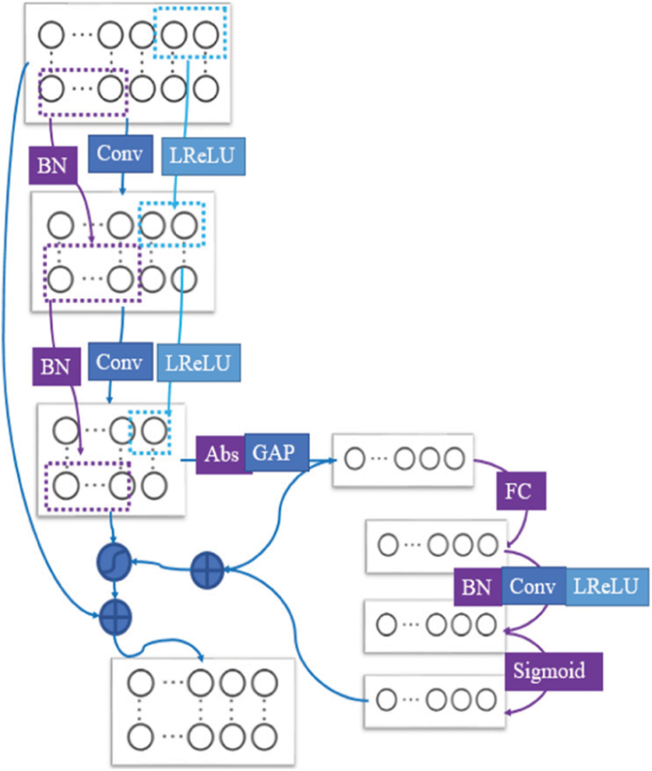
Figure 1: Structure diagram of deep residual shrinkage network
The main purpose of the convolutional layer is to extract features from the input feature graph. Assuming that the bias parameter of the convolution layer
The function of the batch normalization layer (BN) is to present the input data to a standard normal distribution. The neural network parameters can be adjusted at a faster convergence rate by always maintaining a larger gradient state. In addition, the batch standardization layer is also used to improve the anti-noise ability of the model [24]. The BN mathematical expression is as follows:
where
The most common activation function is rectified linear unit (ReLU). However, the ReLU will abandon the characteristics of vibration signals when the input is a negative bearing signal, which weakens the performance of the model in rolling bearing fault diagnosis. Therefore, the Leaky rectified linear unit (LReLU) is used in this paper. The mathematical expression is as follows:
where
The role of the pooling layer is to reduce the size of input data. The mathematical expression is as follows:
where
The residual block structure is shown in Fig. 2. The BN and LReLU are located before the convolution layer so that the input can be directly connected to the output across the multi-layer network, which is more conducive to parameter training. Assuming that multiple residual blocks are stacked, the forward transmission of information from the residual block
where
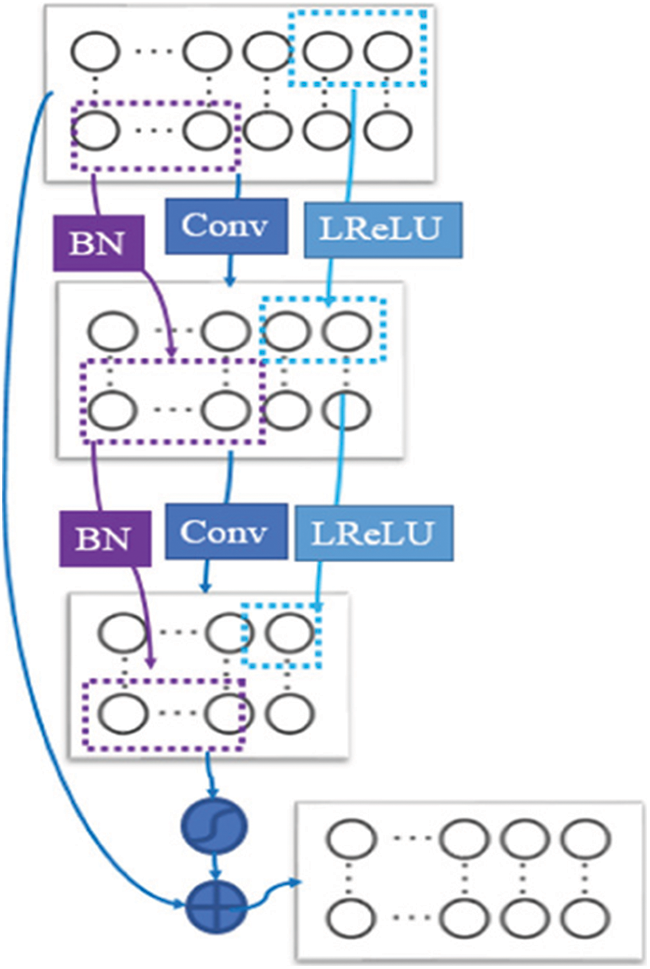
Figure 2: Schematic diagram of residual block structure
Soft threshold is a function that shrink the input data towards zero. It is often used in signal denoising algorithms. The formula is as follows:
where
The Softmax layer is used for the output of multiple categories and the mathematical expression is as follows:
3 Bearing Fault Diagnosis Model Based on Improved Anti-Noise Residual Shrinkage Network
In this paper, the deep residual shrinkage network is improved to ensure the accuracy of the fault diagnosis model considering the noisy environment in the actual industry. In order to improve the feature extraction ability of the model, the convolution layer in the deep residual shrinkage network is replaced by a Dense-Net layer. The first layer of the model is set as the Drop-block layer to further improve the noise resistance ability of the model.
The basic function of the Drop-block layer is to add noise to the neural network. It mainly contains two parameters, one is the size of the region to be removed and the other controls the amount of data to be removed.
Vincent et al. [25] proposed a de-noising auto-encoder that the idea of which is to zero the original data according to a certain probability, encode and decode the obtained data and obtain the restored data. This can reduce the sensitivity of the network to noise interference and has better feature extraction, expression ability and stronger robustness. This article uses the same idea and sets the first layer after model input as the Drop-block layer.
A part of the adjacent continuous signal of the whole piece in the signal is removed through the Drop-block layer and the model will pay attention to other important characteristics of the signal to achieve correct classification to obtain better generalization. At the same time, this is similar to the data set enhancement technology. By removing some signals following a certain distribution, the number of training samples is added to maximize the versatility of the neural connection, reduce the overfitting of the neural network and enhance the anti-noise ability of the model.
3.2 Improved Residual Shrinkage Layer
The residual shrinkage layer introduces the soft threshold value into the residual module and uses the method of adaptive threshold setting to suppress the noise in the signal and the features considered useless to the current classification. Meanwhile, as shown in Fig. 3, this paper replaces the convolutional layer in the deep residual shrinkage network with a Dense-Net to improve the ability of the model extract fault features in a high-noise environment. The Dense-Net layer structure is shown in Fig. 4.
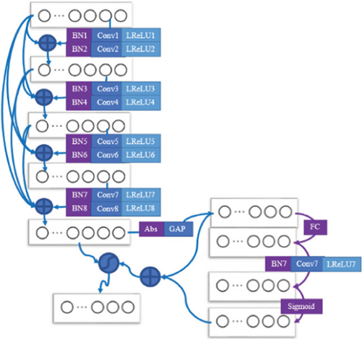
Figure 3: Improved schematic diagram of residual shrinkage layer
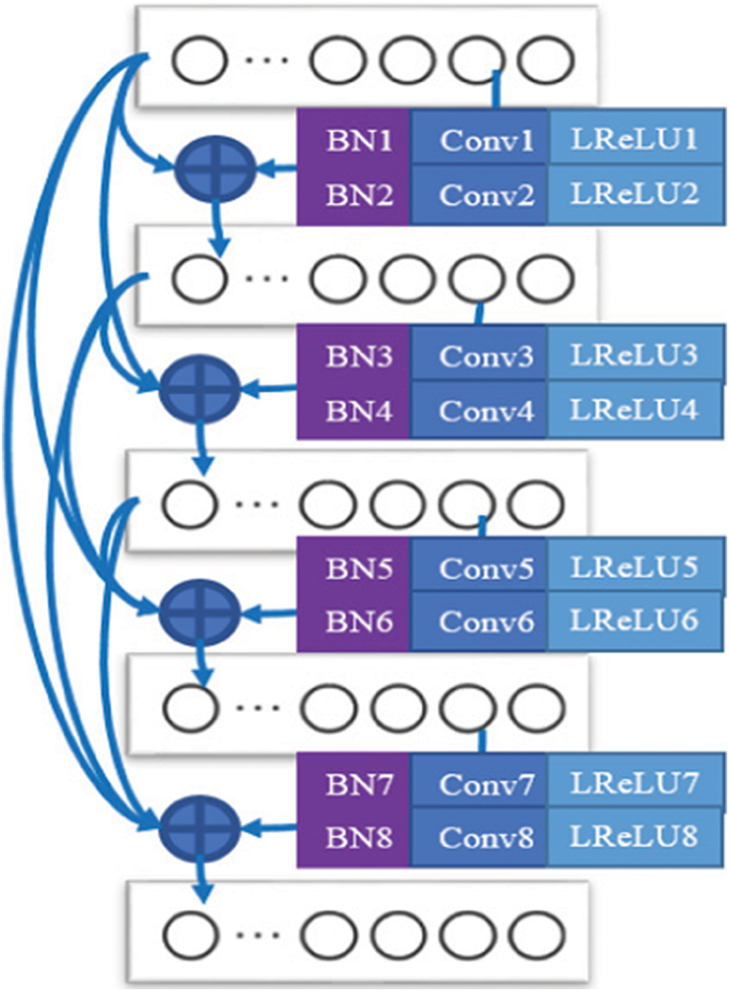
Figure 4: Schematic diagram of Dense-Net layer structure
Finally, the bearing fault diagnosis model of the wind turbine can be constructed and its structure is shown in Fig. 5. First, the original signal is preprocessed to obtain the bearing signal samples with labeling. Then, an improved deep residual shrinkage network bearing fault diagnosis model is trained based on the labeled bearing samples. In the fault diagnosis model, the first layer of the model is set as the Drop-block layer and the convolution layer in the deep residual shrinkage network is replaced by the Dense-Net module. Finally, the labeled training set data samples are input into the model for training and the trained model is applied to the test set to output fault diagnosis results.
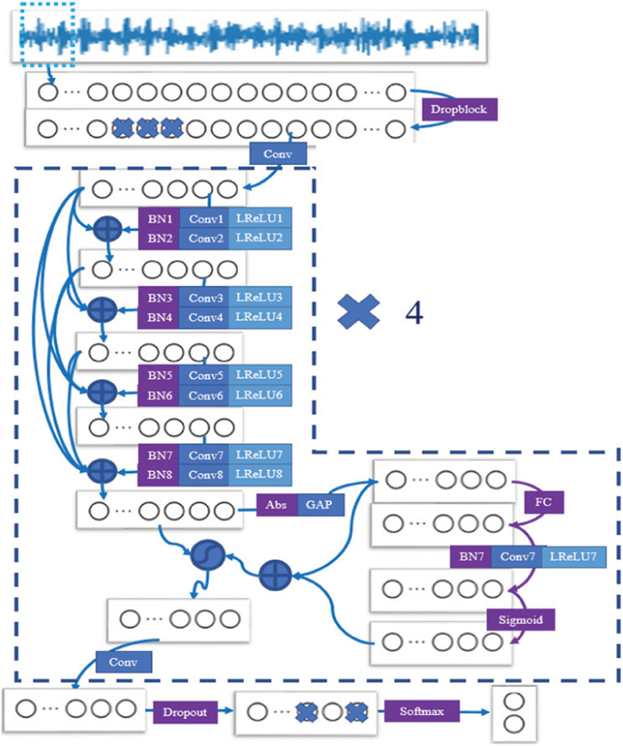
Figure 5: Schematic diagram of bearing fault diagnosis model
In this section, fault data and normal data of rolling bearings of wind turbines are used to verify the effectiveness of the proposed fault diagnosis model. First, the training and test samples were captured from the originally collected signals. Then, the bearing fault diagnosis model of the wind turbine was build based on the improved anti-noise residual shrinkage network. Finally, the results of the trained fault diagnosis model are compared with other methods.
The experimental data were obtained from a 1.5 MW wind turbine in a wind field. The locations of sensor measurement points are shown in Fig. 6, which mainly includes seven measuring points that include mainshaft bearing, input end of gearbox, inner gear ring of gearbox, low-speed shafts in gearbox, high speed shaft output of gearbox, the drive end of generator and the free end of generator. In this paper, two types of data are selected: faulty samples and normal samples. Each type of sample contains 500 samples, and the sampling frequency and length of each sample are 5120 Hz and 4096, respectively. The proportion of training and test sets is 5:1 and white noise with a random signal-to-noise ratio is added to the test set to test the noise resistance of the model. The data of the sample used for verification in the experiment came from the measuring point 6 which fault type was the outer ring fault of the rear bearing of the generator. The time-domain waveform and spectrum of fault vibration data are shown in Fig. 7.
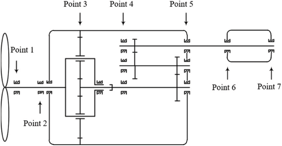
Figure 6: Schematic diagram of sensor measurement point layout
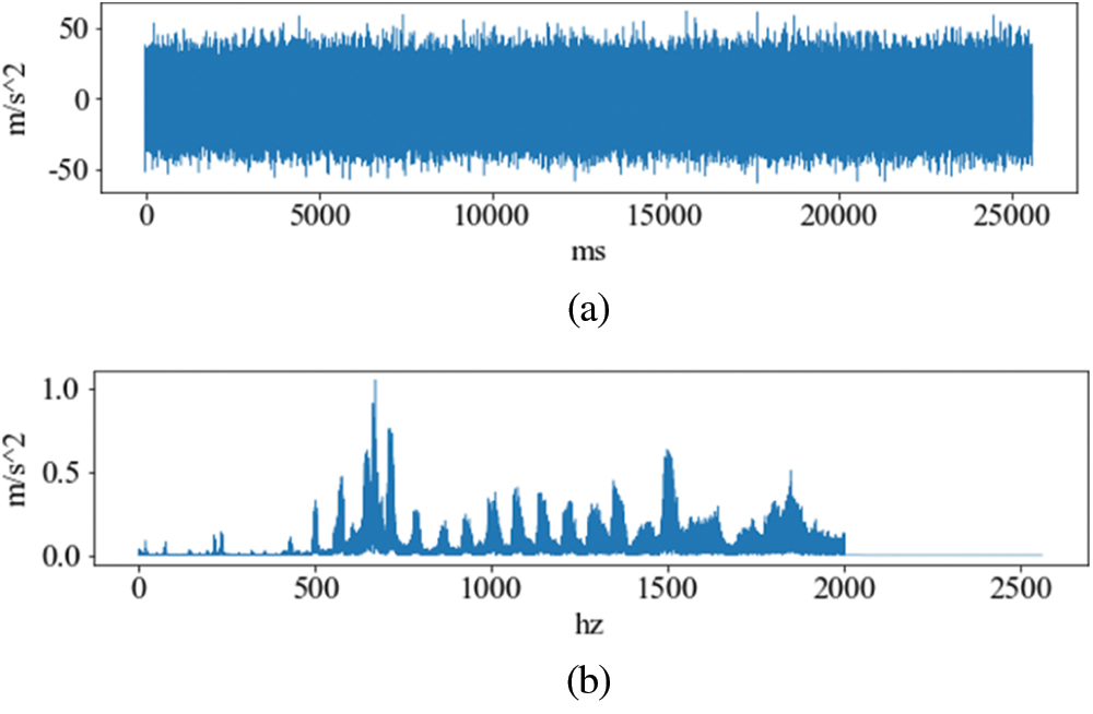
Figure 7: The time domain and frequency domain waveforms of fault samples. (a) The time domain waveform (b) The frequency domain waveform
4.2 Improved the Structural Parameters of the Residual Shrinkage Network Model
The parameters of each layer of the improved anti-noise residual shrinkage network are shown in Table 1. The fault diagnosis model used in this experiment consists of one Drop-block layer, four convolution layers, four improved residual shrinkage layers, one Dropout layer, one GAP layer and one SoftMax layer. The network model used in the experiment is Python and Tensorflow platforms.
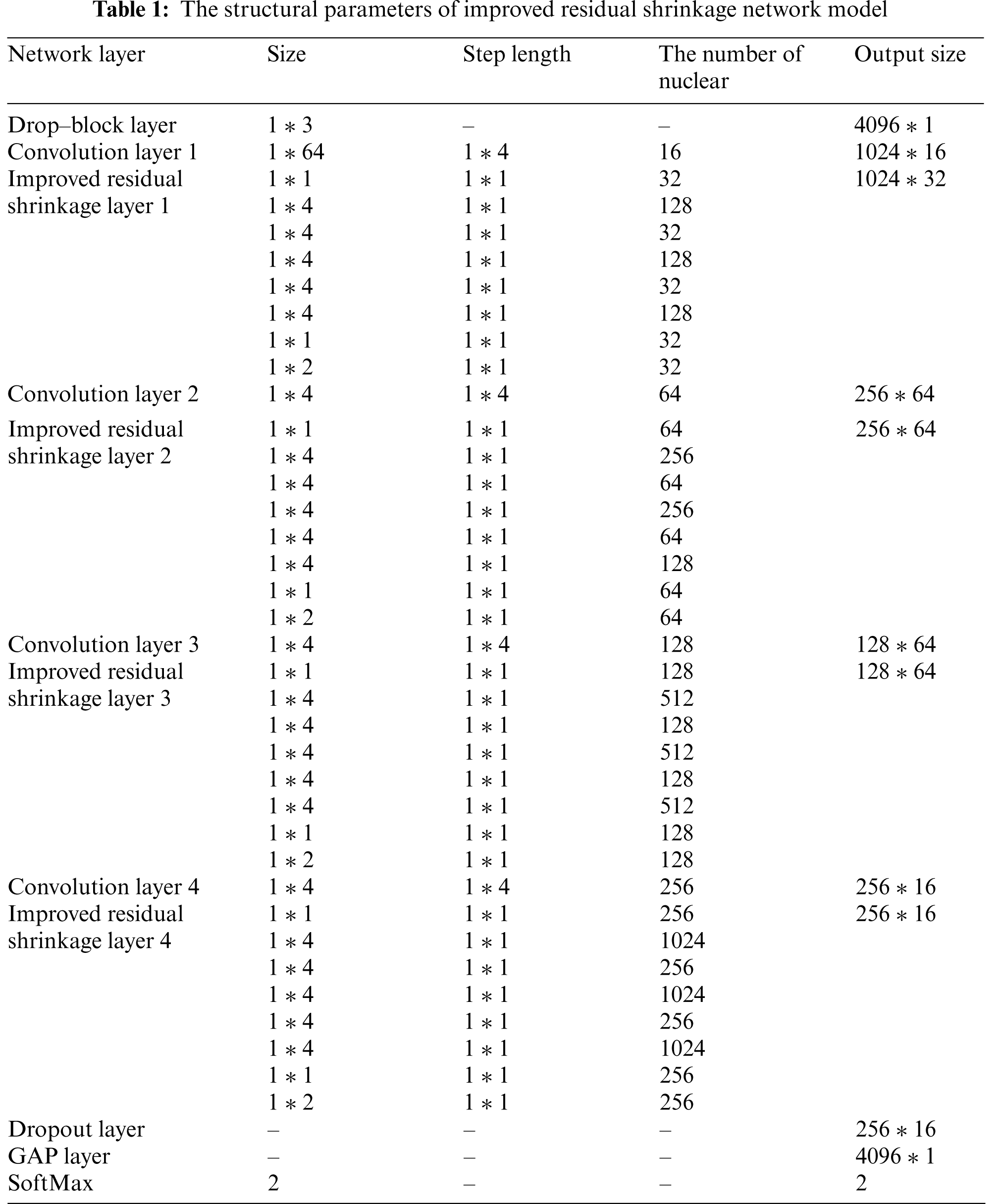
The size of the first convolution kernel is 1 * 64 [26], which has a certain anti-interference effect. A Dense-Net structure is adopted in the improved residual shrinkage layer. The depth of the convolution kernel is gradually increased, which makes the enhanced model more capable of extracting complex features and better applicable to the noise environment. The size of the convolution kernel of the remaining convolution layer is 1 * 4. The activation function is LReLU, which can retain part of the bearing signal characteristics from the negative half axis and is more suitable for bearing signals. The pooling type is average pooling. The batch normalization after each convolution layer to improve the performance of the model and accelerate the convergence of the model.
In order to better display the feature extraction effect of the model in this paper, distributed stochastic neighbor embedding (t-SNE) is applied to reflect the distribution characteristic of the test sample as it passes through each of the modified residual shrinkage layers that is shown Fig. 8. In the Fig. 8, the blue is the normal sample and the purple is the fault sample. First, as shown in Fig. 8, features are indivisible in the early layers and become more and more separable as the layers get deeper and deeper. It is note that these features are easily divided although there are a small number of misclassified samples in the last few layer. Then, as you can see from the visualization in Fig. 8a, the feature representation of the input is evenly distributed, but subsequent layers of features gradually coming together. Finally, there are two parts in the failure sample, which may be caused by further deterioration of the failure.
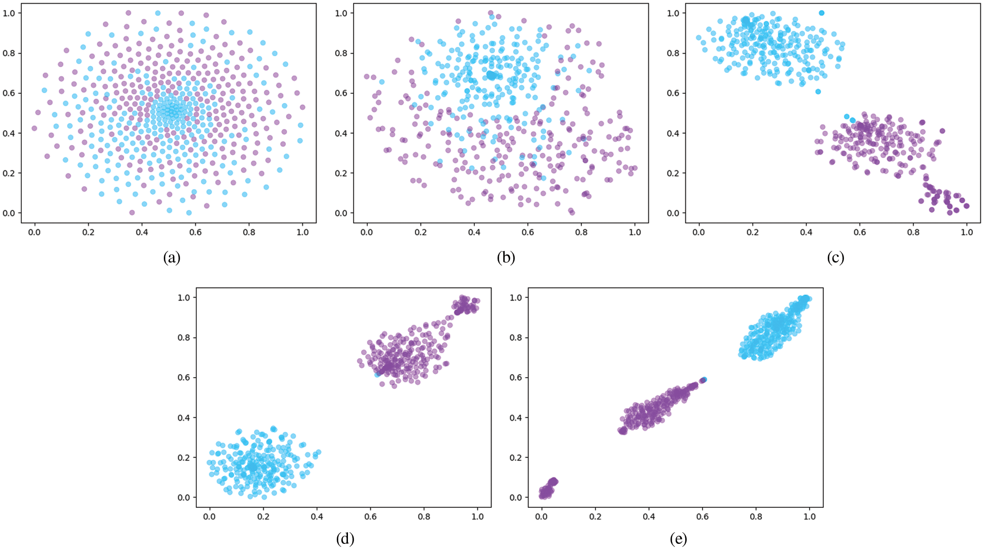
Figure 8: The characteristic distribution diagram of test samples. (a) Input layer (b) Shrinkage layer 1 (c) Shrinkage layer 2 (d) Shrinkage layer 3 (e) Shrinkage layer 4
In this section, the performance of different models in different signal-to-noise ratio environments is compared through controlled experiments to verify the role of different modules in the model. In order to validate each improved module of the model proposed in this paper, three models are set up for comparison in the experiment. Table 2 compares the diagnostic accuracy of test sets of different models under different noise environments. In Table 2, Model A represents the proposed method with an improved structure of the anti-noise residual shrinkage network model. The first layer is the Drop-block layer and the residual shrinkage layer contains the Dense-Net layer, whose structural parameters are shown in Table 1. Model B represents the original convolution layer that is the original residual shrinkage network that the Dense-Net layer are removed from the proposed model. The first layer is the Drop-block layer and the structure of other parameters is consistent with Model A. Model C implies that the Drop-block layer is removed from the proposed model and the Dense--Net layer is included in the residual shrinkage layer. The structure of other parameters is consistent with Model A.
As shown in Table 2, the diagnostic accuracy of the three models increases with the increase of signal-to-noise ratio. When the signal-to-noise ratio reaches 0 dB, all models show high accuracy. The diagnostic accuracy can reach more than 99% that the normal and fault can be distinguished. Compared with Models B and C, Model A is the most stable. When the signal-to-noise ratio of model A rises from −10 to 0 dB, the accuracy rate rises from 89.24% to 99.75%, which is only a 10% increase. However, the signal-to-noise ratio of Models B and C increases from 60% to 99%; the accuracy rate rises only by 40%, which reflects the stability of the improved model proposed in this paper in the noise environment. At the same time, the average diagnostic accuracy of Model A is 13.47% higher than that of Model B and 8.16% higher than that of Model C under the noise environment from −10 to 0 dB. In conclusion, the improved model proposed has certain advantages of good anti-noise ability and fault diagnosis ability in a noisy environment.
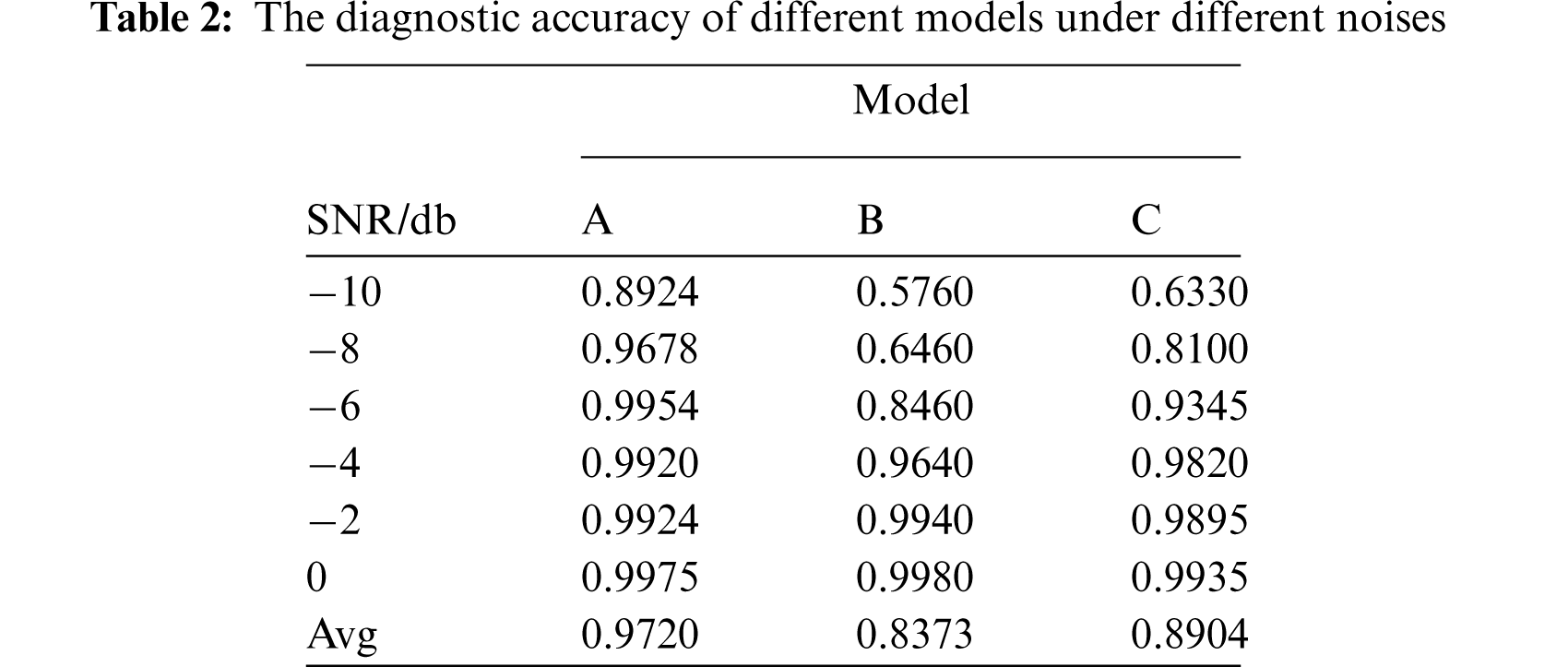
Compared with Model B, the diagnostic accuracy of Model A is higher than that of Model B in the high noise environment, which is 31.64% higher in the −10 dB environment, 32.18% higher in the −8 dB environment and there is little difference in the diagnostic accuracy of the two models in the −2 dB environment, which shows that the Dense-Net layer can help the model obtain more effective features in a high noise environment and thus achieve better fault diagnosis.
Similarly, compared with Model C, the diagnostic accuracy of Model A is higher than Model C in the signal-to-noise ratio environment from −10 to 0 dB, which indicates that the Drop-block layer as the first layer of the model can effectively improve the diagnostic accuracy of the model in a noisy environment and enable the model to obtain better anti-noise performance. It also shows that adding random interference to the original signal can effectively prevent overfitting of the training model, which results in better performance of the model in a high-noise environment.
In summary, the control experiments of the three models effectively verified the good performance of the proposed model in a noisy environment and validated the effectiveness of the improved Dense-Net layer and Drop-block layer in the model.
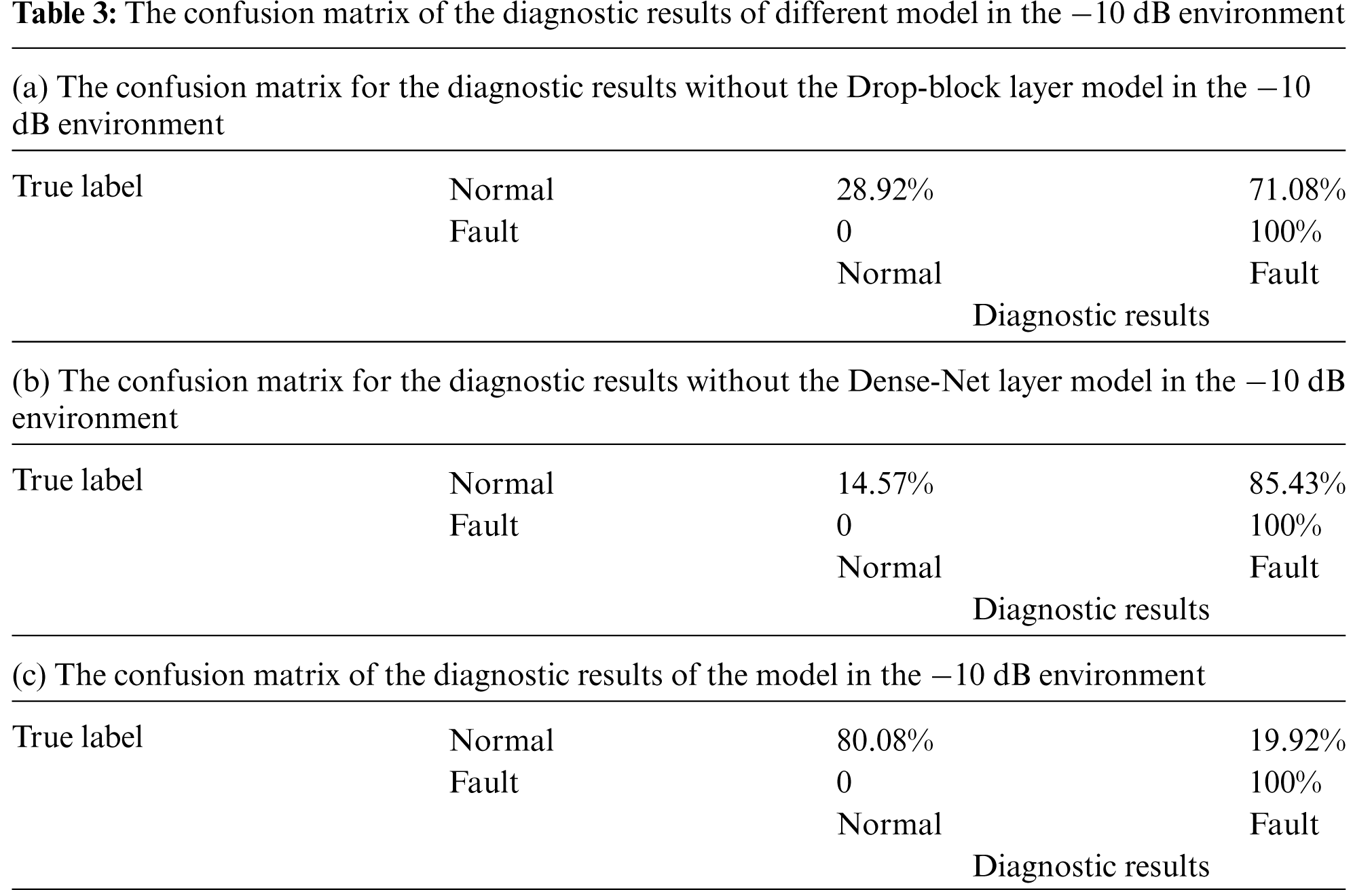
In order to further discuss the role of the Dense-Net layer and Drop-block layer, the diagnostic results of the three models at −10 dB were analyzed using a confusion matrix. Tables 3a–3c show the confusion matrix of diagnostic results of the model without the Drop-block layer, the model without the Dense-Net layer and the model in this paper, respectively. The abscissa of the confusion matrix is the diagnostic result of the test data and the ordinate is the true label of the test data. The percentage in each cell is the distribution of diagnostic results for each model for each real category of test data.
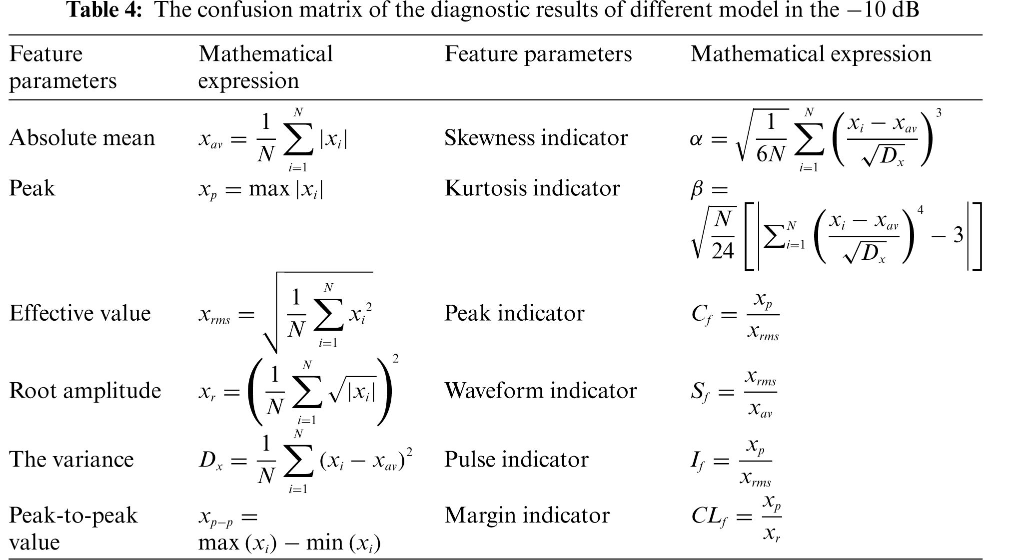
The accuracy of bearing fault diagnosis by SVM, DNN, CNN and DEDCNN [27] models in the −10 dB environment is shown in Fig. 9. The kernel function selected by SVM is the RBF function. The input characteristics of SVM are common time-frequency characteristics. The detailed feature information is shown in Table 4. The
From the comparison results in Fig. 9, it can be seen that the diagnostic accuracy of the method proposed is higher than other methods in the −10 dB environment in this paper. The main reason is that the final result of the traditional SVM method is very dependent on early feature engineering, which needs to make effective features to obtain better results manually and the process requires experience or various attempts. Deep learning is an end-to-end method that automatically extracts effective features and realizes classification. Compared with the other two classical networks of deep learning mentioned method above and the proposed method in the literature [27], the method presented in this paper can better extract the features of the data and has a certain resistance to noise. Therefore, sensitive features can be extracted in a noisy environment and all models can show better diagnosis results.
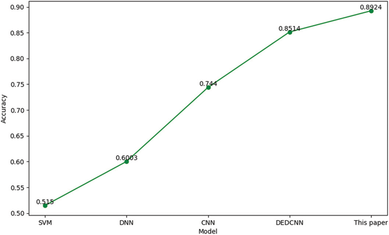
Figure 9: The diagnostic accuracy of different classification models in −10 dB environment
1. In this paper, a new and improved anti-noise residual shrinkage network is developed to meet the requirements of bearing fault diagnosis of the wind turbine in a high noise environment. The model takes the original signal as input and achieves the end-to-end fault diagnosis without manual experience or feature engineering. The proposed improved anti-noise residual shrinkage network can realize fault diagnosis in a noisy environment.
2. There are two structural improvements for noise: Dense-Net layer and Drop-block layer in the residual shrinkage network. The Drop-block layer and Dense-Net layer can help the model obtain more effective features in a high noise environment and make the model more noise tolerance, resulting in a better fault diagnosis effect.
3. Compared with some other models, the verification results show that the proposed improved anti-noise residual shrinkage network has a better anti-interference ability and can better realize the fault diagnosis of wind turbine bearings.
Funding Statement: The authors received no specific funding for this study.
Conflicts of Interest: The authors declare that they have no conflicts of interest to report regarding the present study.
1. Zeng, J., Chen, Y. F., Yang, P., Guo, H. X. (2018). Review on fault diagnosis of large wind turbine. Power System Technology, 42(3), 849–860. DOI 10.13335/j.1000-3673.pst.2017.2311. [Google Scholar] [CrossRef]
2. Li, G., Qi, Y., Li, Y. Q., Zhang, J. F. (2021). Research progress on fault diagnosis and state prediction of wind turbine. Automation of Electric Power System, 45(4), 180–191. DOI 10.7500/AEPS20200301002. [Google Scholar] [CrossRef]
3. Long, X. F., Yang, P., Gong, H. X., Wu, X. W. (2017). Review of fault diagnosis methods for large wind turbine. Power System Technology, 41(11), 3480–3491. DOI 10.13335/j.10003673.pst.2016.3326. [Google Scholar] [CrossRef]
4. Jiang, Y. H., Li, Y. Q., Jiang, W. D., Tang, C., Cai, J. C. et al. (2017). Fault feature extraction method based on EMD and bisspectral analysis. Journal of Vibration, Measurement & Diagnosis, 37(2), 338–342+407. DOI 10.16450/j.cnki.issn.1004-6801.2017.02.021. [Google Scholar] [CrossRef]
5. Feng, Z., Ming, L., Yi, Z., Hou, S. (2012). Fault diagnosis for wind turbine planetary gearboxes via demodulation analysis based on ensemble empirical mode decomposition and energy separation. Renewable Energy, 47(C1), 112–126. DOI 10.1016/j.renene.2012.04.019. [Google Scholar] [CrossRef]
6. Xin, Y., Li, S. M., Wang, J. R., Yi, P. X., Liu, H. (2018). Gear fault diagnosis method based on iterative empirical wavelet transform. Chinese Journal of Scientific Instrument, 39(11), 79–86. DOI 10.19650/j.cnki.cjsi.J1702813. [Google Scholar] [CrossRef]
7. Peng, F. (2010). Sparse signal decomposition method based on multi-scale chirplet and its application to the fault diagnosis of gearboxes. China Mechanical Engineering, 25(7), 549–557. DOI 10.1016/j.ymssp.2010.06.004. [Google Scholar] [CrossRef]
8. Sun, J. Y., Sun, W. L., Xu, H. C. (2018). Research on gear deterioration fault diagnosis of large wind turbine. Machinery Design & Manufacture, 9, 101–104. DOI 10.19356/j.cnki.1001-3997.2018.09.028. [Google Scholar] [CrossRef]
9. Zhu, X. T. (2019). Fault diagnosis of rolling bearing based on kernel principal component analysis and naive Bayes. Modern Computer, 9, 18–22. [Google Scholar]
10. Jurgen, H., Mohammad, H., Ramezani, M., Bach-Andersen, N. L. (2018). Bayesian state prediction of wind turbine bearing failure. Renewable Energy, 116(1), 164–172. DOI 10.1016/j.renene.2017.02.069. [Google Scholar] [CrossRef]
11. Wang, X., Yan, W. Y. (2017). Fault diagnosis of rolling bearing based on variational mode decomposition and SVM. Journal of Vibration and Shock, 36(18), 252–256. DOI 10.13465/j.cnki.jvs.2017.18.037. [Google Scholar] [CrossRef]
12. Wang, Z., Yao, L., Cai, Y. (2020). Rolling bearing fault diagnosis using generalized refined composite multiscale sample entropy and optimized support vector machine. Measurement, 156(1), 107574. DOI 10.1016/j.measurement.2020.107574. [Google Scholar] [CrossRef]
13. Wang, Z., Yao, L., Cai, Y., Zhang, J. (2020). Mahalanobis semi-supervised mapping and beetle antennae search based support vector machine for wind turbine rolling bearings fault diagnosis. Renewable Energy, 155(2), 1312–1327. DOI 10.1016/j.renene.2020.04.041. [Google Scholar] [CrossRef]
14. Wang, Z., Li, G., Yao, L., Qi, X., Zhang, J. (2021). Data-driven fault diagnosis for wind turbines using modified multiscale fluctuation dispersion entropy and cosine pairwise-constrained supervised manifold mapping. Knowledge-Based Systems, 228, 107276. DOI 10.1016/j.knosys.2021.107276. [Google Scholar] [CrossRef]
15. Kong, Y., Qin, Z., Wang, T., Han, Q., Chu, F. (2021). An enhanced sparse representation-based intelligent recognition method for planet bearing fault diagnosis in wind turbines. Renewable Energy, 173(5), 987–1004. DOI 10.1016/j.renene.2021.04.019. [Google Scholar] [CrossRef]
16. Wang, J., Wei, Q., Qu, L. (2018). Wind turbine bearing fault diagnosis based on sparse representation of condition monitoring signals. IEEE Transactions on Industry Applications, 55(2). DOI 10.1109/TIA.2018.2873576. [Google Scholar] [CrossRef]
17. Hoang, D. T., Kang, H. J. (2018). Rolling element bearing fault diagnosis using convolutional neural network and vibration image. Cognitive Systems Research, 53(6), 42–50. DOI 10.1016/j.cogsys.2018.03.002. [Google Scholar] [CrossRef]
18. Han, T., Tian, Z. X., Yin, Z., Tan, A. (2020). Bearing fault identification based on convolutional neural network by different input modes. Journal of the Brazilian Society of Mechanical Sciences and Engineering, 42(9), 719. DOI 10.1007/s40430-020-02561-6. [Google Scholar] [CrossRef]
19. Duan, L., Song, C. Y., Liu, C., Wei, W., Lv, C. J. (2021). Temperature state recognition of high-speed train bearing based on machine learning. Journal of Jilin University (Engineering and Technology Edition), 6, 1–8. DOI 10.13229/j.cnki.jdxbgxb20200751. [Google Scholar] [CrossRef]
20. Lei, Y. G., B., Y., Du, Z. J., Lv, N. (2019). Deep migration diagnosis method for mechanical equipment fault based on big data. Journal of Mechanical Engineering, 55(7), 1–8. DOI 10.3901/JME.2019.07.001. [Google Scholar] [CrossRef]
21. Wei, Z. A., Xiang, L., Qian, D. D. (2019). Deep residual learning-based fault diagnosis method for rotating machinery. ISA Transactions, 95(1–2), 295–305. DOI 10.1016/j.isatra.2018.12.025. [Google Scholar] [CrossRef]
22. Zhao, M., Kang, M., Tang, B., Pecht, M. (2018). Deep residual networks with dynamically weighted wavelet coefficients for fault diagnosis of planetary gearboxes. IEEE Transactions on Industrial Electronics, 65(5), 4290–4300. DOI 10.1109/TIE.2017.2762639. [Google Scholar] [CrossRef]
23. Zhao, M., Zhong, S., Fu, X., Tang, B., Pecht, M. (2020). Deep residual shrinkage networks for fault diagnosis. IEEE Transactions on Industrial Informatics, 16(7). DOI 10.1109/TII.2019.2943898. [Google Scholar] [CrossRef]
24. Kai, Z., Zuo, W., Chen, Y., Meng, D. Y., Zhang, L. (2016). Beyond a gaussian denoiser: Residual learning of deep CNN for image denoising. IEEE Transactions on Image Processing, 26(7), 3142–3155. [Google Scholar]
25. Vincent, P., Larochelle, H., Bengio, Y., Manzagol, P. A. (2008). Extracting and composing robust features with denoising auto-encoders. Proceedings of the Twenty-Fifth International Conference, pp. 1096–1103. Helsinki, Finland [Google Scholar]
26. Wei, Z., Peng, G., Li, C., Chen, Y., Zhang, C. (2017). A new deep learning model for fault diagnosis with good anti-noise and domain adaptation ability on raw vibration signals. Sensors, 17(3), 425. DOI 10.3390/s17020425. [Google Scholar] [CrossRef]
27. Wu, Z. H., Jiang, H. K., Liu, S. W., Zhao, K. E. (2021). A deep ensemble dense convolutional neural network for rolling bearing fault diagnosis. Measurement Science and Technology, 32(10), 104014. DOI 10.1088/1361-6501/ac05f5. [Google Scholar] [CrossRef]
 | This work is licensed under a Creative Commons Attribution 4.0 International License, which permits unrestricted use, distribution, and reproduction in any medium, provided the original work is properly cited. |