Energy Engineering

DOI: 10.32604/ee.2022.017471

ARTICLE

A New Diagnostic Method Applied to Gearbox Missing Gear Faults ——LOD-ICA

Lida Liao1, Bo Xiao1,2,*, Kan Huang1,*, Bin Huang1,3 and Kang Zhang1

1Changsha University of Science & Technology, Changsha, 410114, China
2China Construction Eighth Engineering Bureau Limited, Tianjin, 200122, China
3University of South Australia, Adelaide, SA 369977, Australia
*Corresponding Author: Bo Xiao. Email: XiaoBo6662021@163.com
Received: 13 May 2021; Accepted: 04 September 2021

1  Introduction

With global warming, the demand for carbon emissions is becoming more and more stringent. The vigorous use of traditional energy sources such as coal, natural gas and oil has seriously aggravated the greenhouse effect and carbon emissions, so the development of clean energy sources has become a major trend in the world [1]. The share of energy in power generation has increased from 9.3% to 10.4% and surpassed nuclear power for the first time in 2019 [2]. Among the various renewable energy sources, wind energy is the fastest growing source of electricity today.

As an important clean energy source, wind energy is the fastest growing source of electricity today. In the past two decades, wind energy has grown by leaps and bounds to become a clean, cost-competitive mainstream energy source worldwide, with 60.4 GW of global wind energy capacity installed in 2019, a 19% increase over the amount installed in 2018, the second best year in history for wind energy development [3]. Wind power is also becoming increasingly important as a share of renewable energy generation: global onshore and offshore wind power accounts for more than 19.1% (or 622,408 MW) of total renewable energy generation, which is only the total capacity (1,263,914 GWH) [4].

As an important tool for wind power generation, wind turbines play a key role in converting wind energy into electricity. When a wind turbine malfunctions, it greatly reduces the power generation, reduces the efficiency of power generation and even shutdown. Therefore, it is essential to diagnose the faults of wind turbines. When a rotating machine fails, it usually generates vibration signals that are neither linear nor steady-state. In contrast, traditional time-frequency analysis methods are more suitable than time-domain or frequency-domain analysis methods for the fault diagnosis of rotating machines [5,6].

However, some traditional methods of time-frequency analysis have proven to be inherently flawed. For example, Fast Fourier transform [7], Wigner-Ville distribution [8] and wavelet transform [9], as they are not adaptive, limit their further development in the field of gearbox fault diagnosis. Empirical mode decomposition (EMD) [10] and local mean decomposition (LMD) [11] are methods of self-adaptive time-frequency based analysis of signal extremes, which are widely used in the field of rotating machinery fault diagnosis [12,13]. However, both decomposition methods are still deficient; the EMD method generates end effects [14], overshoots and undershoots [15], pattern mixing [16], and unexplained negative frequencies generated by the Hilbert transform [17], etc. The LMD method also suffers from local mutations and even large computational size due to the sliding iterative computation method, which increase the probability of the LMD method generating modal mixing problems [18,19]. Recently, Zhang et al. proposed a new time-frequency analytical technique for adaptively decomposable signals—local oscillatory-characteristic decomposition (LOD), based on the LMD method [20]. The LOD method processes the vibration signal by means of differential transformation, coordinate domain transformation, and segmented linear transformation, and decomposes the original signal into several single mono-oscillation components (MOCs) with the LOD signal. The LOD method improves the computational efficiency of the LMD method, which has a large computational volume. The LOD method ameliorates the problem of large computational volume of the LMD method, and greatly improves the computational efficiency. For this reason, the LOD method has been extensively used in the area of rotating machinery fault diagnosis since it was proposed [21,22]. Compared with the LOD method, the LOD method based on noise-assisted analysis effectively improves the modal mixing problem of mixed fault signals. However, with the scholars’ in-depth study, it is found that the LOD method based on noise-assisted analysis still has the same problems as the LMD method, EMD method and LOD method. That is, the LOD method based on noise-assisted analysis also has the problem of signal modal mixing and cannot achieve complete separation of signals.

After the LOD algorithm processing, the MOC component of the single-component signal generated by the decomposition of the rotating machinery and equipment will be affected by external factors such as the mixing of other signals in the field during the actual operation of the machinery, as well as internal factors such as the defects of the LOD method itself, causing the MOC component to contain more than one fluctuation mode characteristics, so that the instantaneous frequency of the MOC component loses its actual physical meaning. Therefore, the instantaneous frequency of the MOC component loses its physical meaning, and the modal mixing problem arises in the signal decomposition processing.

Independent Component Analysis (ICA) is a good way to deal with the signal-mode mixing problem [23]. Due to this property, the ICA algorithm is extensively applied to the processing of blind source separation problems for mixed acoustic signals [24,25]. However, the ICA algorithm is often limited by the insufficient number of observation channels, which limits the further development of the ICA method. The fast ICA method has received wide attention because of its faster convergence and higher computational speed than the classical ICA algorithm [26]. However, the fast ICA algorithm also often limits the further development of the method because of the insufficient number of observation channels.

In this paper, a new method of self-adaptive temporal-frequency is proposed, namely the LOD-ICA method. The method combines the advantages of both noise assisted analysis based LOD and fast ICA methods to make up for the respective defects of the two methods to achieve vibration signal processing. The algorithm first preprocesses the observed signal by the LOD algorithm based on noise-assisted analysis to improve enough virtual channel data for the fast ICA algorithm; and then uses the fast ICA algorithm to achieve complete signal separation to meet the real-time monitoring of rotating machinery and realize fault diagnosis. The rest of the paper is structured as below. The LOD method and its inherent drawbacks are reviewed in Section 2. Section 3 describes in detail the working principle of the LOD-ICA method and the main steps of the LOD-ICA method as well as the evaluation criteria. Section 4 discusses the comparison between the LOD-ICA method and the LOD method based on noise-assisted analysis in the analysis of analog signals. Section 5 presents the results of vibration signal analysis of wind turbine gearbox faults, and Section 6 gives the conclusions of this paper.

2  LOD Method Based on Noise-Assisted Analysis and Its Disadvantages

A The local oscillation characteristic decomposition (LOD) method is essentially a new approach to the oscillation signal for temporal and frequency analysis to achieve an adaptive decomposition of the oscillation signal in order to get a series of single oscillation components (MOCs) and a residual based on the local extremum points of the signal. The LOD method contains three basic operations: the derivative operation, the operation of transformation of the axial domain and the operation of segmental rectangular transformation [27]. However, in practice, the shortcomings of the LOD method's own decomposition capability, as well as the influence of external factors such as sampling frequency, intermittent signals, etc., can lead to the occurrence of signal modal mixing. That is, the same MOC component contains different fluctuation modes, or the same fluctuation mode is decomposed into different MOC components, losing the real physical meaning of the signal.

Based on this, the white noise is added to the LOD method to assist the analysis by referring to the improvement of the EMD method to the EEMD method. After adding white noise to the target signal, each time scale of the signal can be uniformly distributed in the passband of the determined filter set, which obviously reduces the interference of the high-frequency intermittent signal to the LOD decomposition method, and the differential operation in the decomposition process can amplify the local fluctuation characteristics of the signal, so that the high-frequency intermittent signal is completely decomposed. Therefore, the addition of white-noise to the target signal, followed by the decomposition of the signal with the LOD method, alleviates the modal mixing problem to a limited extent. The following LOD method based on noise-assisted analysis is used to decompose and calculate a set of multicomponent AM-FM simulation signals x(t):

x1(t)=4sin(7πt)×sin⁡(1520πt)(1)

x2(t)=2sin(300πt)(2)

x3(t)=3sin(42πt)(3)

x4(t)=4sin(180πt)(4)

x(t)=x1(t)+x2(t)+x3(t)+x4(t)(5)

In Eqs. (1) to (5), t∈[0,0.5], the sampling frequency of the simulated signal is set to 4096 Hz; from Eq. (5), it can be seen that the simulated signal x(t) is composed of a modulated signal x1(t) and three other sinusoidal signals x2(t), x3(t), x4(t). The time frequency waveforms of the analog signal x(t) and four of its components x1(t), x2(t), x3(t) and x4(t) are presented in Fig. 1 below. The FFT profiles of the analog signal x(t) as well as its components are shown in Fig. 2, while Figs. 3 and 4 show respectively a time-frequency plot and the FFT profile of the analog signal x(t) after decomposing based on the LOD method of noise-assisted analysis.

Figure 1: Time-domain waveforms of the analog signal x(t) with its components

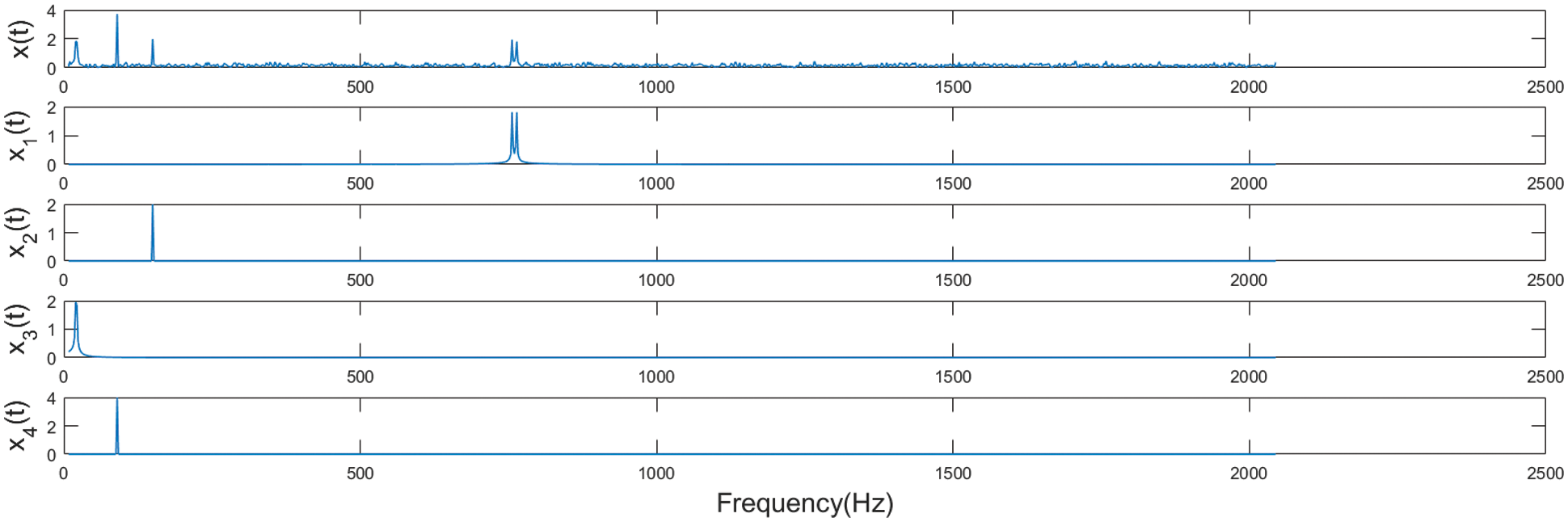
Figure 2: FFT spectrum for analog signal x(t) with its components

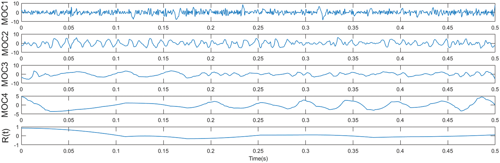
Figure 3: Time-frequency diagram of LOD decomposition results based on noise-assisted analysis

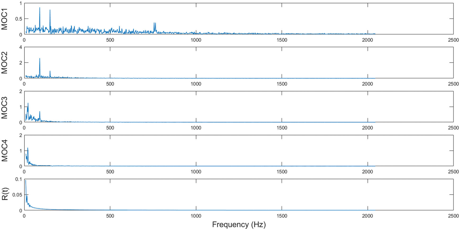
Figure 4: FFT spectrum of LOD decomposition results based on noise-assisted analysis

As shown in Fig. 3, the original signal x(t) is decomposed into four MOC components and one residue, where the four MOC components correspond to the four signal components x1(t), x2(t), x3(t) and x4(t), respectively. From Figs. 3 and 4, it can be seen that the signal is decomposed by the LOD method with adaptive noise-assisted analysis based on the decomposition process, which reflects its basic characteristics. The spectrum generated by the fast Fourier transform of the simulated signal after decomposition based on the LOD method of noise-assisted analysis (Fig. 4) is analyzed in comparison with the fast Fourier transform spectrum of the simulated signal (2), which shows that the MOC1 component generated by the decomposition based on the LOD method of noise-assisted analysis is not completely decomposed and its instantaneous frequency is not physically meaningful. The FastICA algorithm can achieve good results when dealing with the modal mixing of signals. Therefore, the aim of this study is to introduce the ICA algorithm to solve the modal mixing problem generated after the signal has been decomposed by the LOD based on noise-assisted analysis and to achieve blind source separation of the original signal.

3  Design Implementation of LOD-ICA Algorithm

3.1 Fast Independent Component Analysis Method

According to the contents of Section 2, it is known that the independent component analysis algorithm can separate the source signal without knowing both the signal channel and the source signal parameters. Also the ICA method satisfies the non-Gaussian distribution, and the separated source signals are independent of each other and uncorrelated [28]. Compared with the traditional ICA method, FastICA method has received more attention and far-reaching research due to its simpler calculation method and faster convergence, and has been widely used in the area of acoustic signature analysis.

The FastICA method, also called fixed immobile point iterative optimization algorithm, achieves the minimization estimation of the non-Gaussianity of the separated signal components by employing a negative entropy objective function to complete the batch processing of mixed signal data. Thus, the definition expression of the FastICA method based on the negative entropy of the nonlinear function is as follows:

Y=wTZ(6)

J(Y)≈(E(G(Y)−E(G(V))))2(7)

In Eq. (6), Y is a random variable normalized (i.e., σY=1,Y¯=0) and Y represents the corresponding signal separated by independent component analysis; w represents a unit vector; Z is the transformation matrix after normalization and whitening of the observed mixed signal X. In Eq. (7), G represents a non-quadratic function that can arbitrarily actually exist; also, V is a random variable with Gaussianity after normalization (i.e., σV=1,V¯=0).

According to the constraints of Lagrangian, it is known that the constraint of E(G(Y)) by the formula E(Y)2=‖w‖2=1 makes E(G(Y)) obtain the extreme value and obtain the optimal solution. Meanwhile, the above case holds then the Lagrangian multiplicative gradient needs to be equal to 0, i.e.,

E(Zg(Y))+βw=0(8)

In Eq. (8), the g function is then the derivative of the function G; β is a constant value of the coefficient. When the solution process of Eq. (8) is carried out by Newton's iterative method, usually the part of E(Zg(Y))+βw in Eq. (8) will be expressed by F, then its gradient relation equation has the following expression:

∂F∂w=E(ZZTg′(Y))+βI(9)

Since the observed mixed signal is the data after already spherical, E(ZZTg′(Y)) in Eq. (9) can be approximated as follows:

E(ZZTg′(Y))≈E(ZZT)+E(g′(Y))=E(g′(Y))I(10)

By the simplification of Eq. (10), the inverse of the matrix is more convenient. Therefore, we can derive the approximate Newton's iteration formula, which is expressed as follows:

w∗←w−[E(Zg(Y))+βw]/[E(g′(Y))+β](11)

In Eq. (11), w∗ is the updated value of w. A simplified treatment of Eq. (10) yields

w∗←E(Zg(Y))−E(g′(Y))w(12)

w=w∗/‖w∗‖(13)

When separating mixed signals using Fsat independent component analysis, two basic conditions must be met: ① The number of test signal channels is at least as large as that of the signal source; ② the original signal must be statistically autonomous from among themselves, and at most one channel of the generator signal may be Gaussian distributed.

3.2 ICA-LOD Method

On the basis of the above, the fast ICA method could be used to separate the signal from the independent, nonlinearly correlated source signal and solve the signal modal mixing problem. Therefore, the paper proposes a new method combining LOD and ICA on the basis of noise-assisted analysis-LOD-ICA method. For a given original signal, the LOD-ICA method operates as follows:

(1) Find all extreme values Xk(k=1,2,…,m) for signal x(t) and its correlative moment value τk, and perform a linear transformation of x(t) between any two neighboring polar values [Xk,Xk+1) to obtain the segmented linear function s1(t). where the linear transformation formula is:

s1(t)=Xk+(Xk+1−Xk)t−τkτk+1−τk

k=1,2,…,M−1(14)

A coordinate transform is used to convert (t,x) to sawtooth domain coordinates (u,s), to decrease the disassembly error. The coordinate transformation formula is:

u(t)=τk+(t−τk)x(t)−XkXk+1−Xkt∈[τk,τk+1)

k=1,2,…,M−1(15)

s(u)=x(t)(16)

From Eqs. (15) and (16), It can be seen that the transformation of the coordinate domain doesn't alter the magnitude of the signature (vertical coordinates), however, just compress or expand the time-axis (horizontal coordinate). This increases the data density at the signal extremes and improves the decomposition accuracy of local features without affecting the time and space of the algorithm.

(2) The first-order differential differentiation of the target signal x(t) is performed to obtain x′(t), and the white noise signal is added to x′(t). The extreme case of x′(t) corresponds to the moments of τk(k=1,2,…,N) and the function value of Xk′ in the original signal x(t) corresponding to the moment value of τk is found, and then the initial mean function m1(u) is linearly connected to Xk′ in the sawtooth domain by the linear transformation. The formula for the linear transformation is.

m1(u)=Xk′+(Xk+1′−Xk′)u−τk′τk+1′−τk′

k=1,2,…,N−1(17)

(3) Subtracting the sawtooth domain s1(u) of the original signal from the sawtooth domain mean function m1(u) yields c1(u) as a high-frequency fluctuation function.

c1(u)=s1(u)−m1(u)(18)

(4) Inverse the coordinates of c1(u) from the sawtooth domain to the original data domain c1(t). where the inverse conversion formula is:

t(u)=τk′+(t−τk′)Xk+1−Xkx(t)−Xku∈[τk′,τk+1′)

k=1,2,…,N−1(19)

c1(t)=c1(τk′)+(c1(u)−c1(τk′))τk+1′−τk′t−τk′t∈[τk′,τk+1′)

k=1,2,…,N−1(20)

Ideally, if c1(t) is a single component signal with a physically meaningful instantaneous frequency, then c1(t) is the first MOC component of x(t)MOC1(t).

(5) If c1(t) is not a physically meaningful instantaneous frequency single component signal, we should repeat the above process m times until cm(t) is a physically meaningful instantaneous frequency single component signal. Then cm(t) will be the first component of the original signal, MOC1(t).

(6) The derived MOC1(t) is then subtracted from the original signal x(t) to obtain the new function r1(t). Treat r1(t) as the new original signal, and repeat (1) through (5) until rn(t) is a monotone function. Thus x(t) gets discretized as the sum with n MOCs as well as the residual rn(t). That is:

x(t)=∑p=1n⁡MOCp(t)+rn(t)(21)

(7) Finally, the generated MOC components are separated by the ICA algorithm to obtain independent and uncorrelated source signals, and signal frequency characteristics are obtained.

The process flow diagram of LOD-ICA approach follows the Fig. 5 below.

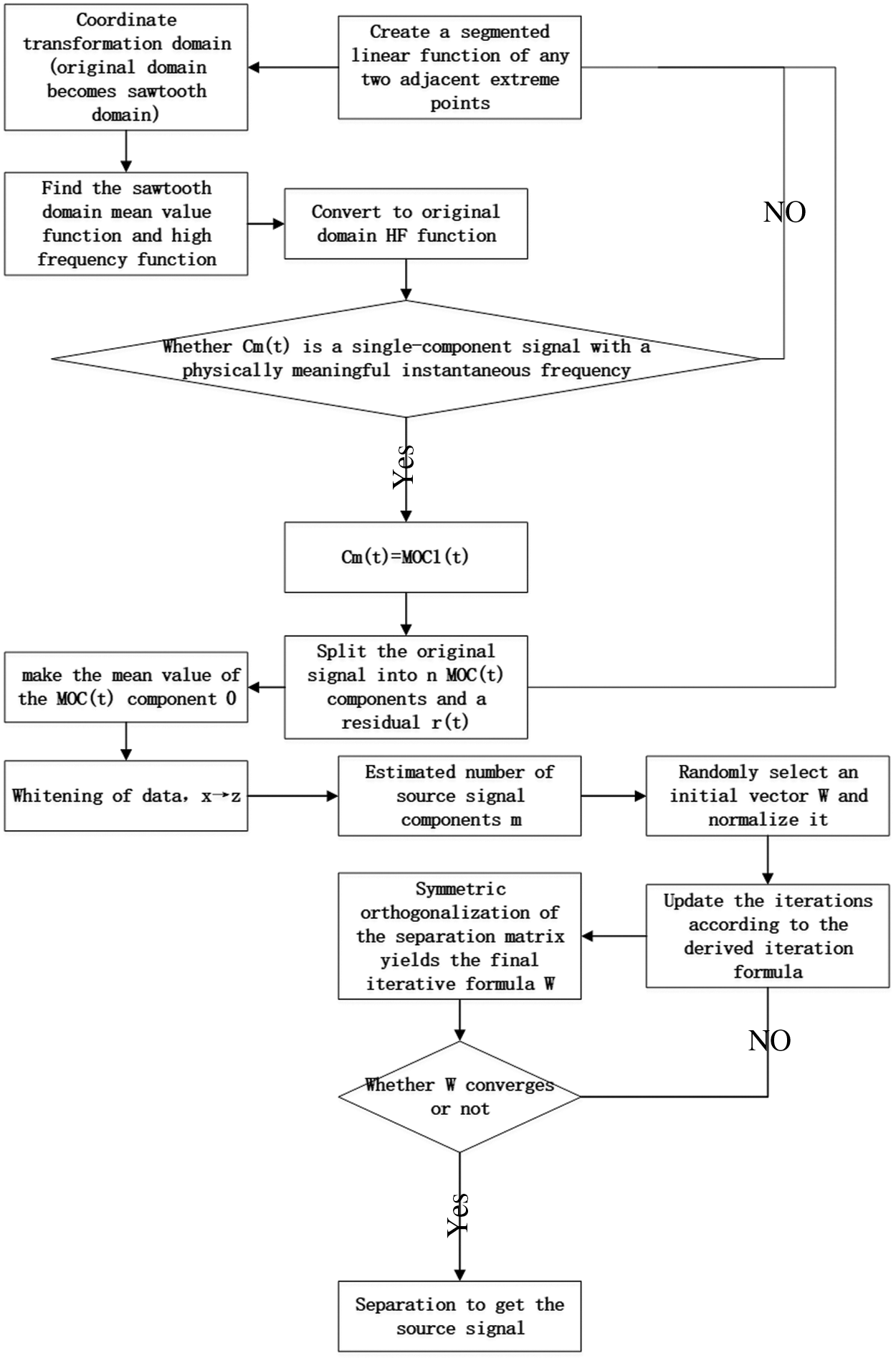
Figure 5: Flow chart of LOD-ICA method

3.3 Evaluation Criteria Based on Correlation Coefficient

In the LOD-ICA method to deal with mixed signal fault feature extraction problem, for the waveform diagram and image signal generated after data processing, we can only make a simple qualitative analysis, which is only a rough judgment of the success of the observed mixed signal separation, and lacks a precise judgment of the mixed signal separation results. And non-Gaussianity is an important judgment basis for the mixed signal analysis results processed by LOD-ICA method, so in this paper, we make a precise judgment of the analysis results based on the measure of correlation coefficient, and analyze them quantitatively. The correlation coefficients are expressed as follows:

ξij=ξ(yi,Sj)=|∑i=1N⁡yi(t)Sj(t)|∑i=1N⁡yi2(t)∑j=1N⁡yj2(t)(22)

In Eq. (22), yi is the separated estimated signal, Sj is the original signal, and the value range of ξij is (0, 1). When ξij = 1, it means that the i-th decomposed estimated signal is identical to the j-th original signal; however, it does not exist in the actual signal decomposition operation, so ξij = 1 exists only in the ideal case. In the actual decomposition operation, the closer the value of the correlation coefficient ξij is to 1, the better the decomposition of the mixed signal is; on the contrary, the closer the value of the correlation coefficient ξij is to 0, the worse the decomposition of the mixed signal is, which means that the mixed signal separation is less successful.

4  Analog Signal Analysis

The same simulation signal as the LOD approach with noise-assisted diagnosis is used in order to verify the effectiveness of the LOD-ICA method and to compare the analysis with the LOD approach with noise-assisted diagnosis.

x1(t)=4(1+2cos⁡(8πt))cos⁡(800πt)(23)

x2(t)=2sin(300πt)(24)

x3(t)=2in(25πt)(25)

x4(t)=4sin(180πt)(26)

x(t)=x1(t)+x2(t)+x3(t)+x4(t)(27)

In Eqs. (23) to (27), t∈[0,0.5], the sampling frequency of the simulated signal is set to 4096 Hz; from Eq. (27), it can be seen that the simulated signal x(t) is composed of a modulated signal x1(t) and three other sinusoidal signals x2(t), x3(t), x4(t). The time domain waveforms and FFT spectra for both the emulated signal x(t) and its four components x_2(t), x_3(t) and x_4(t) are shown as follows in Figs. 6 and 7, respectively. The resultant time-frequency plot and FFT decomposition spectrum after decomposing the simulated signal x(t) by the noise-assisted analysis-based LOD method are also shown as follows in Figs. 8 and 9, respectively. From Figs. 6–9, it can be seen that the basic characteristics of the simulated signal, based on the noise-assisted analysis of the LOD decomposition of the simulated signal into four MOC components and one residue. By comparing the two groups in Fig. 6 with Figs. 8 and 7 with Fig. 9, it can be seen that after the decomposition of LOD with the addition of white noise, the signal mixing phenomenon still exists between MOC1-MOC4, and their instantaneous frequencies are not physically meaningful, and the simulated signal does not achieve complete separation. Therefore, the LOD approach is still subject to signal mixing problems with the noise-assisted analysis.

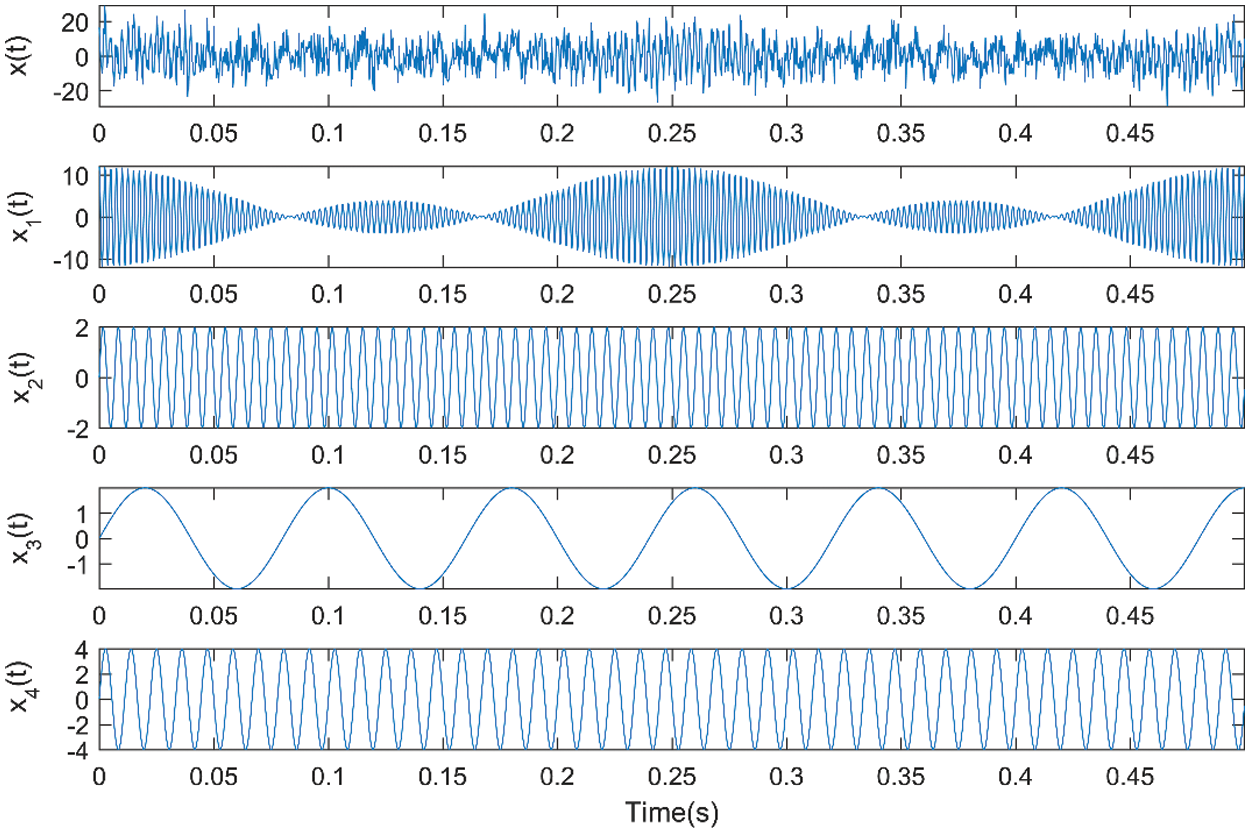
Figure 6: Time-domain waveforms for the analog signal x(t) and components thereof

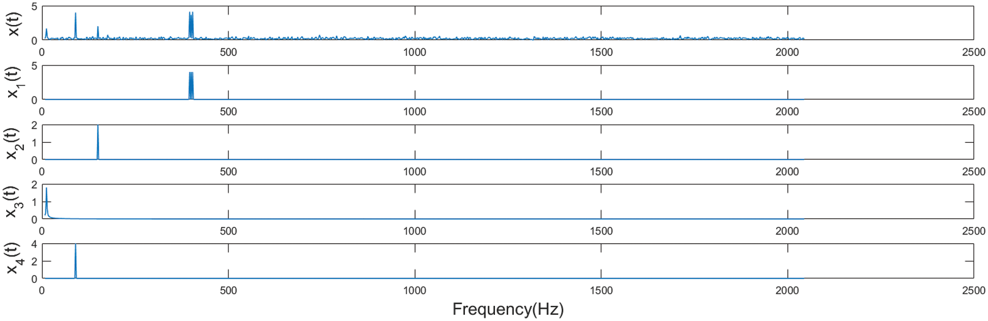
Figure 7: Simulated FFT series of the signal x(t) and its components

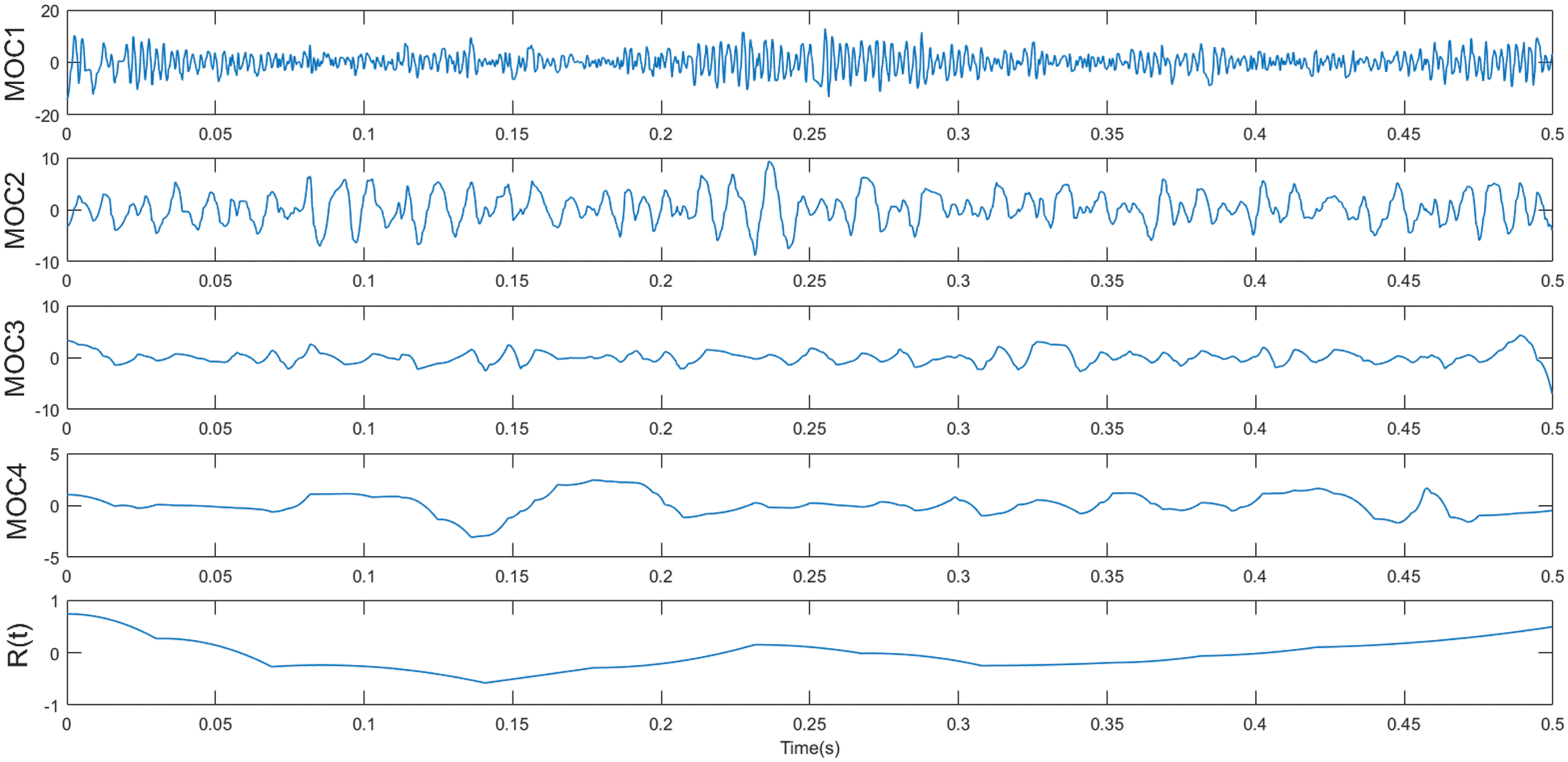
Figure 8: Time-frequency diagram of LOD decomposition results based on noise-assisted analysis

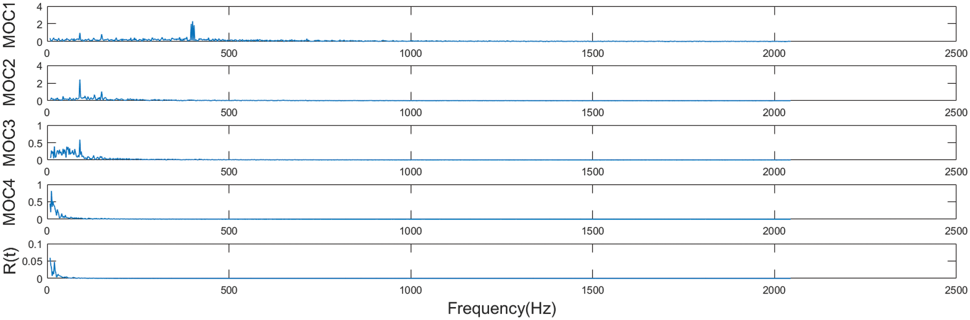
Figure 9: Spectrogram of LOD decomposition results based on noise-assisted analysis

Because the LOD method with the addition of white noise fails to completely decompose the signal, the blind source separation is performed for the signals that fail to be completely decomposed. After pre-processing the mixed signals with the LOD approach on the basis of noise-assisted interpretation, the separation is continued with the fast ICA method, as shown in Fig. 10-figure supplement 11 below. Figs. 10 and 11 show the signal component time-frequency and spectrum plots at the fast ICA algorithm partitioning, respectively.

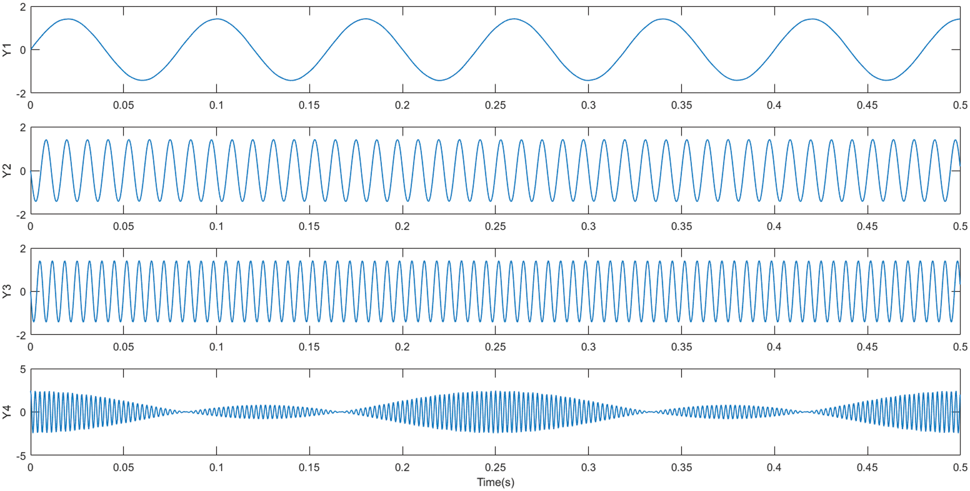
Figure 10: Fast ICA decomposition time-frequency diagram of simulated signal components

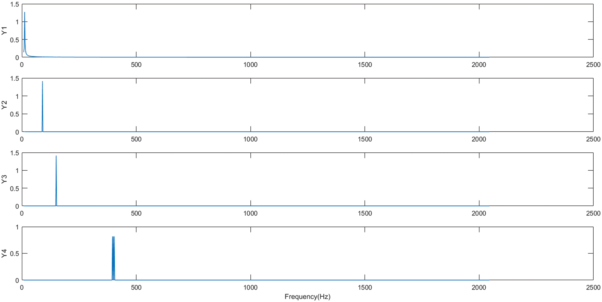
Figure 11: Fast ICA decomposition spectrogram of simulated signal components

As can be seen from Figs. 10 and 11, the mixed signal components are processed by the fast ICA method to separate the high-frequency signal from the low-frequency signal, and the four separated components Y1, Y2, Y3 and Y4 are all single-component signals with the same fluctuation mode, and the analog signal is completely separated and restored. The mixed signal waveform is separated by the fast ICA method, and the blind source separation of the mixed signal is achieved, and the simulated signal characteristics are successfully extracted.

After calculation, the correlation coefficients of the signal components decomposed by the LOD method based on the noise-assisted analysis and the analog signal components are:

ξ11=0.714905290222428,ξ22=0.531571949047849,

ξ34=0.625202799918692,ξ43=0.757920229431253;

And the correlation coefficients of the signal components decomposed by the LOD-ICA method and the analog signal components are:

ξ14=0.999998785948666,ξ23=0.999999817962504,

ξ31=0.999951160444155,ξ42=0.999999460181505.

According to the comparison of the values of correlation coefficients taken, 1<ξLOD−ICA<ξLOD<0. That is, the signal components decomposed by the LOD-ICA method are more correlated with the original analog signal.

Therefore, the new LOD-ICA method, which is generated by combining the LOD method with the fast ICA method with the addition of white noise, has better results in mixed signal feature extraction compared with the LOD method with the addition of white noise, and can completely separate the mixed signal, restore the source signal as highly as possible, and successfully extract the features of the faulty signal.

5  Application in Gearbox Missing Gear Fault Feature Extraction

When large rotating machinery and equipment fail, the generated vibration signal is usually non-stationary and non-linear. The LOD-ICA method firstly uses the LOD method based on noise assisted analysis to pre-process the original signal, which is decomposed into several MOC components, each single component instantaneous frequency has physical significance; then the independent signal components are sorted out by the fast ICA method to solve the signal mixing problem; finally, the fault features are extracted from the oscillatory signals to complete the fault diagnosis. the LOD-ICA method is particularly applicable to the fault diagnosis of rotating machinery. Therefore, this paper applies the LOD-ICA method to wind turbine gearbox missing gear fault feature extraction in order to prove the effectiveness of the method.

The planetary gearbox system consists of a 100-tooth gear ring, four parallel-distributed 36-tooth planetary gears and a planetary carrier as shown in Fig. 12. The axis of solar wheel is in the same line with the gear ring, and the axis of the four planetary gearboxes is fixed on the planetary carrier. Star wheels are mounted on this planetary carrier, and the planetary gears can rotate around their own axis, and can rotate along the planetary shelf with the planetary gears, i.e., the planetary gears both rotate and rotate along the axis of the planetary shelf. This test bench's planetary gearbox simulates the types of failures of planetary gearboxes in real wind turbines. Fig. 12a and 12b show the normal gearbox and the missing gearbox, and this experiment simulates the gearbox failure in the missing gearbox.

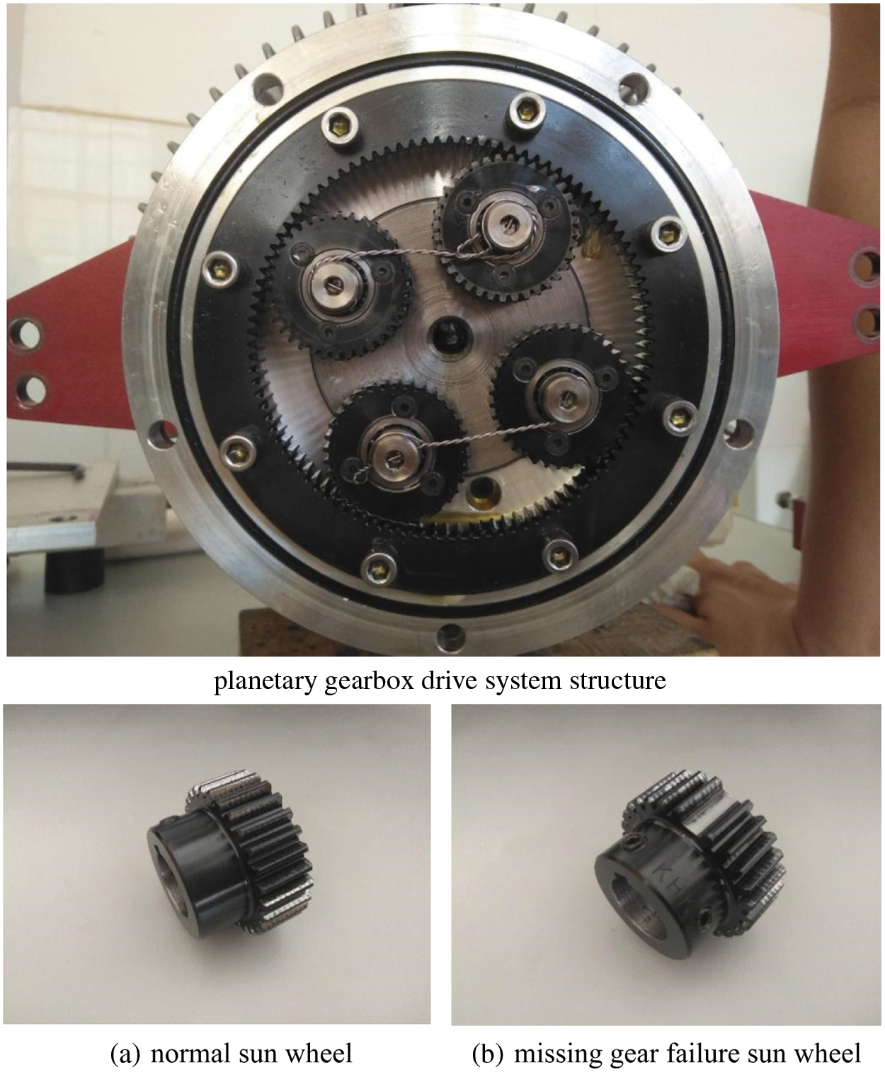
Figure 12: Planetary gearbox

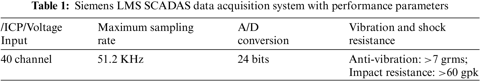
Sound signals were collected by an LMS SCADAS datalogger equipped with a Danish B&K 4189-1/2” microphone with a sampling frequency of 51,200 Hz, described in Fig. 13. Details of the dimensions of the Siemens LMS SCADAS datalogger are shown by way of Table 1.

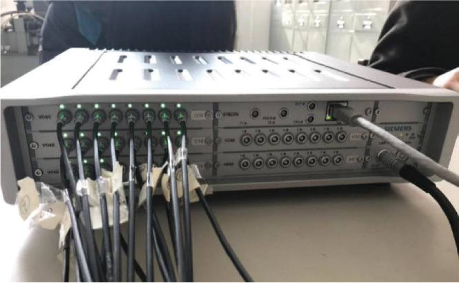
Figure 13: Siemens LMS SCADAS for data collection systems

The source signal used in this experiment is the audio signal of the gearbox gear missing gear fault, with a sampling frequency of 12800 Hz and 396800 sampling points. The waveform (Fig. 14) and spectrum (Fig. 15) of the original signal were obtained from the acquired gear fault signal, and the results of the experimental simulation signal are as follows.

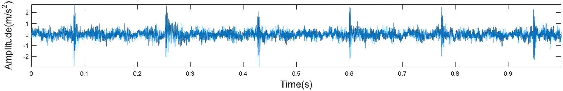
Figure 14: Time domain waveform of vibration signal for gearbox gear fault diagnosis

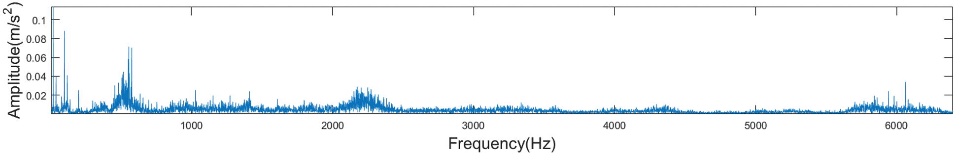
Figure 15: Vibration signal spectrum for gearbox gear fault diagnosis

The original experimental signal was decomposed by the LOD method with the addition of white noise, and the decomposition results were as follows.

Among them, Fig. 16 illustrates the temporal-frequency diagram based on the noise-assisted analysis of the gearbox out-of-gear fault signal after LOD decomposition, and Fig. 17 shows the spectral plot of the gearbox missing gear fault signal decomposed by LOD based on noise-assisted analysis. Figs. 16 and 17 show the decomposition of the fault vibration signal into seven MOC components and one residue by the LOD method with the addition of white noise. From the comparison of the two figures, it can be seen that the decomposition of the four components MOC1, MOC2, MOC3 and MOC4 in the signal of the main frequency band from 1000 to 3000 Hz is not complete, so their instantaneous frequencies do not have practical physical meaning, and the noise-assisted analysis based LOD approach still suffers from signal mixing.

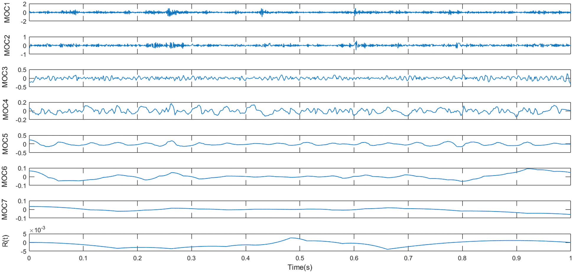
Figure 16: Time-frequency diagram of LOD decomposition of fault signals based on noise-assisted analysis

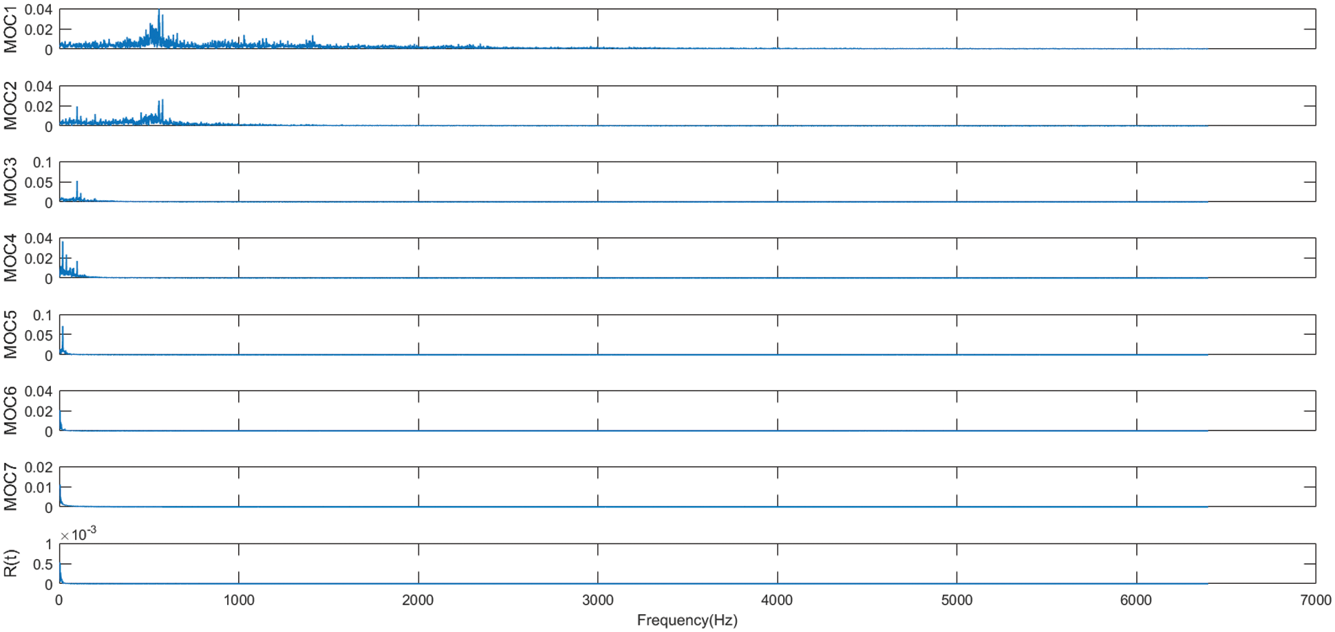
Figure 17: LOD decomposition spectrogram of fault signal based on noise assisted analysis

The undecomposed component signals are introduced into the fast ICA calculation method, and the blind source separation of mixed signals is achieved by transforming between linear transformation matrices. The decomposition results are shown in the following figure.

Figs. 18 and 19 show the fast ICA decomposition time-frequency and spectrum plots obtained from the mixed signal after pre-processing ( the source signal has a mean value of 0 and a variance of 1), respectively. From the above figure, it is clear that the waveform of the mixed signal is well separated and restored, and the fault feature extraction of the signal is finally realized.

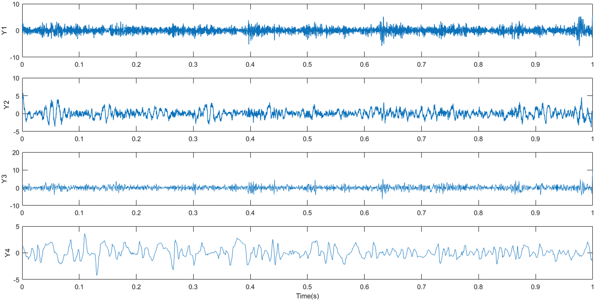
Figure 18: Fast ICA decomposition time-frequency diagram of mixed signal components

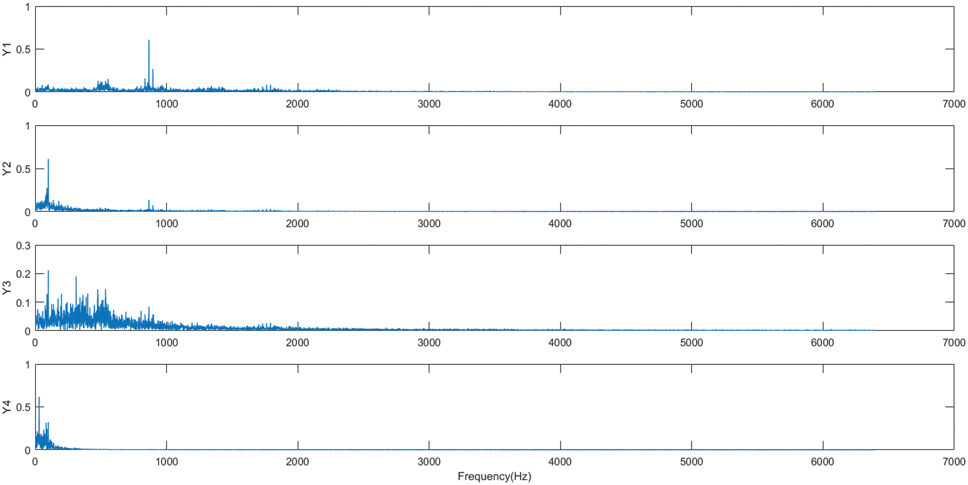
Figure 19: Fast ICA spectrogram for mixed signal components

6  Conclusion

Excessive emissions of carbon substances have become a concern, and the use of traditional energy sources has exacerbated the problem of carbon emissions, so there is an urgent need for a renewable and clean energy source to alleviate the carbon emission problem. With the increasing utilization of wind energy in renewable energy sources, wind turbines, as the key component for converting wind energy into electricity, failures greatly reduce the power generation efficiency or even shut down. Therefore, this paper makes a study on a new method for fault diagnosis of wind turbine gearboxes in order to expect more efficient and stable operation of wind turbines.

However, the LOD method based on noise-assisted analysis to deal with faulty vibration signals generates signal modal mixing problems when gearboxes have missing gear faults. The fast ICA method is very suitable for dealing with the blind source separation problem of acoustic signals, but its requirement for the number of data channels is very high. Therefore, this paper combines the LOD method with the ICA method and proposes the LOD-ICA method. And the method is used for feature extraction of rotating machinery fault diagnosis. The conclusions obtained are as follows:

1.    Through simulated signal analysis, it has been compared that the LOD-ICA method takes into account the advantages of both the LOD with added white noise and the fast ICA method, with high computational speed, short decomposition time, low number of iterations, and no obvious end effect. The fast ICA algorithm is introduced for resolving the signal modal mixing problem generated by the LOD method in processing signals which is assisted by noise based analysis to ensure that each source signal is independent and uncorrelated with each other. And according to the comparison of correlation coefficients, it is found that the LOD-ICA method is better than the LOD method based on noise-assisted analysis in the decomposition of mixed signals.

2.    The analysis of the experimental signal of the fan gearbox missing gear fault indicates that the signal is pre-processed using the LOD method with the addition of white noise, and then processed by the fast ICA method, which not only improves the signal processing speed, but also accurately identifies the characteristic frequencies and maintains good measurement accuracy, and the source signal waveforms are well separated and restored. the LOD-ICA approach could obtain the feature information from the oscillation signal effectively, and is more suitable for gearbox missing gear fault feature extraction than the LOD method based on noise assisted analysis.

Funding Statement: The authors received no specific funding for this study.

Conflicts of Interest: The authors declare that we have no conflicts of interest to report regarding the present study.

References

 1.  Luo, X., Wang, J., Dooner, M., Clarke, J. (2015). Overview of current development in electrical energy storage technologies and the application potential in power system operation. Applied Energy, 137, 511–536. DOI 10.1016/j.apenergy.2014.09.081. [Google Scholar] [CrossRef]

 2.  Dudley, B. (2018). BP statistical review of world energy. London, UK. [Google Scholar]

 3.  GWEC Market Intelligence. Global Wind Report 2019. http://gwec.net/global-wind-report-2019/. [Google Scholar]

 4.  IRENA. (2019). https://www.irena.org/Statistics/View-Data-by-Topic/Capacityand-Generation/Statistics-Time-Series. [Google Scholar]

 5.  Yang, Y., Dong, X., Peng, Z., Zhang, W., Meng, G. (2015). Vibration signal analysis using parameterized time–frequency method for features extraction of varying-speed rotary machinery. Journal of Sound & Vibration, 335, 350–366. DOI 10.1016/j.jsv.2014.09.025. [Google Scholar] [CrossRef]

 6.  Prudhom, A., Jose, A. A., Hubert, R., Vicente, C. A. (2017). Time-frequency vibration analysis for the detection of motor damages caused by bearing currents. Mechanical Systems & Signal Processing, 84, 747–762. DOI 10.1016/j.ymssp.2015.12.008. [Google Scholar] [CrossRef]

 7.  Fadi, A. B., Sunar, M., Cheded, L. (2011). Vibration analysis of rotating machinery using time–frequency analysis and wavelet techniques. Mechanical Systems and Signal Processing, 25(6), 2083–2101. DOI 10.1016/j.ymssp.2011.01.017. [Google Scholar] [CrossRef]

 8.  Li, H., Zhang, Q., Qin, X., Sun, Y. (2020). K-SVD-based WVD enhancement algorithm for planetary gearbox fault diagnosis under a CNN framework. Measurement Science and Technology, 31(2), 025003. DOI 10.1088/1361-6501/ab4488. [Google Scholar] [CrossRef]

 9.  Ma, P., Zhang, H., Fan, W., Wang, C. (2019). Early fault diagnosis of bearing based on frequency band extraction and improved tunable Q-factor wavelet transform. Measurement, 137, 189–202. DOI 10.1016/j.measurement.2019.01.036. [Google Scholar] [CrossRef]

10. Zhang, Y., Tang, B., Xiao, X. (2016). Time–frequency interpretation of multi-frequency signal from rotating machinery using an improved Hilbert–Huang transform. Measurement, 82, 221–239. DOI 10.1016/j.measurement.2016.01.001. [Google Scholar] [CrossRef]

11. Ma, J., Wu, J., Wang, X. (2018). A hybrid fault diagnosis method based on singular value difference spectrum denoising and local mean decomposition for rolling bearing. Journal of Low Frequency Noise, Vibration and Active Control, 37(4), 928–954. DOI 10.1177/1461348418765973. [Google Scholar] [CrossRef]

12. Lei, Y., Lin, J., He, Z., Zuo, M. J. (2013). A review on empirical mode decomposition in fault diagnosis of rotating machinery. Mechanical Systems and Signal Processing, 35(1–2), 108–126. DOI 10.1016/j.ymssp.2012.09.015. [Google Scholar] [CrossRef]

13. Cheng, G., Li, H., Hu, X., Chen, X., Liu, H. (2017). Fault diagnosis of gearbox based on local mean decomposition and discrete hidden Markov models. Proceedings of the Institution of Mechanical Engineers, Part C: Journal of Mechanical Engineering Science, 231(14), 2706–2717. DOI 10.1177/0954406216638885. [Google Scholar] [CrossRef]

14. Wolszczak, P., Łygas, K., Litak, G. (2017). Monitoring of cutting conditions with the empirical mode decomposition. Advances in Science & Technology Research Journal, 11, 96–103. DOI 10.12913/22998624/68467. [Google Scholar] [CrossRef]

15. He, Z., Shen, Y., Wang, Q. (2012). Boundary extension for Hilbert–Huang transform inspired by gray prediction model. Signal Processing, 92, 685–697. DOI 10.1016/j.sigpro.2011.09.010. [Google Scholar] [CrossRef]

16. Lei, Y., Lin, J., He, Z., Zuo, M. (2013). A review on empirical mode decomposition in fault diagnosis of rotating machinery. Mechanical Systems & Signal Processing, 35, 108–126. DOI 10.1016/j.ymssp.2012.09.015. [Google Scholar] [CrossRef]

17. Zheng, J., Cheng, J., Yang, Y. (2014). Partly ensemble empirical mode decomposition: An improved noise-assisted method for eliminating mode mixing. Signal Processing, 96, 362–374. DOI 10.1016/j.sigpro.2013.09.013. [Google Scholar] [CrossRef]

18. Sheng, J., Dong, S., Liu, Z., Gao, H. (2016). Fault feature extraction method based on local mean decomposition Shannon entropy and improved kernel principal component analysis model. Advances in Mechanical Engineering, 8(8), 1687814016661087. DOI 10.1177/1687814016661087. [Google Scholar] [CrossRef]

19. Hu, J., Ren, D., Yang, S. (2009). Spline-based local mean decomposition method for vibration signal. Journal of Data Acquisition & Processing, 24, 82–83. DOI 10.1360/972009-1514. [Google Scholar] [CrossRef]

20. Chen, B., He, Z., Chen, X., Cao, H., Cai, G. et al. (2011). A demodulating approach based on local mean decomposition and its applications in mechanical fault diagnosis. Measurement Science & Technology, 22, 055704. DOI 10.1088/0957-0233/22/5/055704. [Google Scholar] [CrossRef]

21. Zhang, K., Shi, Y., Tang, M., Wu, J. (2016). Local oscillatory-characteristic decomposition and its application in roller bearing fault diagnosis. Journal of Vibration & Shock, 35, 89–95. DOI 10.13465/j.cnki.jvs.2016.01.016. [Google Scholar] [CrossRef]

22. Wu, J., Peng, X., Yang, Y., Zhang, K., Cheng, J. (2016). Quantitative diagnosis method of gear cracks based on noise-assisted LOD. China Mechanical Engineering, 27, 3183–3189. DOI 10.3969/j.issn.1004-132X.2016.23.011. [Google Scholar] [CrossRef]

23. Kim, D., Kim, S. K. (2012). Comparing patterns of component loadings: Principal component analysis (PCA) versus independent component analysis (ICA) in analyzing multivariate non-normal data. Behav Res Methods, 44, 1239–1243. DOI 10.3758/s13428-012-0193-1. [Google Scholar] [CrossRef]

24. Feng, L., Zhao, C., Huang, B. (2019). A slow independent component analysis algorithm for time series feature extraction with the concurrent consideration of high-order statistic and slowness. Journal of Process Control, 84, 1–12. DOI 10.1016/j.jprocont.2019.09.005. [Google Scholar] [CrossRef]

25. Knollmüller, J., Enßlin, T. A. (2017). Noisy independent component analysis of auto-correlated components. Physical Review E, 96(4042114. DOI 10.1103/PhysRevE.96.042114. [Google Scholar] [CrossRef]

26. Feng, Y., Li, H. (2020). Dynamic spatial-independent-component-analysis-based abnormality localization for distributed parameter systems. IEEE Transactions on Industrial Informatics, 16(5), 2929–2936. DOI 10.1109/TII.9424. [Google Scholar] [CrossRef]

27. Zhang, K., Chen, X., Liao, L., Tang, M., Wu, J. (2018). A new rotating machinery fault diagnosis method based on local oscillatory-characteristic decomposition. Digital Signal Processing, 78, 98–107. DOI 10.1016/j.dsp.2018.02.018. [Google Scholar] [CrossRef]

28. Pinto, L. S., Assunção, M. V., Ribeiro, D. A., Ferreira, D. D., Huallpa, B. N. et al. (2020). Compression method of power quality disturbances based on independent component analysis and fast Fourier transform. Electric Power Systems Research, 187, 106428. DOI 10.1016/j.epsr.2020.106428. [Google Scholar] [CrossRef]

This work is licensed under a Creative Commons Attribution 4.0 International License, which permits unrestricted use, distribution, and reproduction in any medium, provided the original work is properly cited.