Energy Engineering

DOI: 10.32604/ee.2022.017687

ARTICLE

Distribution Network Equipment Location and Capacity Planning Method Considering Energy Internet Attribute from the Perspective of Life Cycle Cost

Qiang Li1,*, Lei Xue1 and Xia Lin2

1State Grid Shanxi Electric Power Company Economic and Technical Research Institute, Taiyuan, China
2State Grid Shanxi Electric Power Company, Taiyuan, China
*Corresponding Author: Qiang Li. Email: victorlq@163.com
Received: 31 May 2021; Accepted: 06 November 2021

1  Introduction

Under the goal of “carbon peaking and carbon neutralization” in China, the energy interconnected distribution network deeply couples the energy flow, information flow and business flow to form a scientific and reasonable new energy system [1–3]. However, as one of its important key technologies, the equipment location and sizing method of energy interconnected distribution network needs to be deeply studied.

At present, many scholars have studied the location and capacity model of equipment in distribution network. In terms of the location and sizing model based on distributed generation, Jiang et al. [4] optimized the location and sizing of access nodes and capacity for renewable energy, and determined the best location of units. Venkatesan et al. [5] distributed generators and capacitor banks to effectively improve the overall performance of distribution system. On this basis, the optimal location and capacity model is established, and the optimal solution is obtained by using hybrid enhanced gray wolf optimization algorithm and particle swarm optimization algorithm. Liang et al. [6] proposed a multi optimization programming model for the grid with large scale on-grid wind power. Su et al. [7] constructed an optimization model considering economy, network loss and voltage stability, in order to solve the problem of location and capacity of distributed generation, and the optimal Pareto solution is obtained by using fuzzy satisfaction evaluation decision-making method. Other scholars have conducted research on the application of electric vehicles, demand response and other aspects in site selection and capacity determination. Habibi et al. [8] developed a multi-objective optimization model for site selection and capacity allocation of municipal solid waste facilities by considering relevant factors such as cost and greenhouse gas emission. Wang et al. [9] proposed a collaborative planning method for site selection and adjustment of energy station and pipeline network, which effectively reduced the annual cost of the system. Gao et al. [10] involved the compressed air in the operation framework and constructed a location and capacity planning model to solve the intermittent problem of renewable energy power generation. Mortaz et al. [11] proposed an optimal investment planning model for a new type of micro grid with vehicle to grid (V2G) technology. Meng et al. [12] studied the location and capacity of large-scale renewable energy access to the system by using multi-attribute decision-making method. Carrión et al. [13] proposed the optimal location and capacity of grid connected photovoltaic power plants by combining multi-scale analysis and analytic hierarchy process with geographic information system technology and considering environment, terrain, geographical location and climate factors. Nojavan et al. [14] proposed a dual objective optimization model to optimize the location and scale of energy storage system (ESS) in microgrid in the presence of demand response program (DRP). Cetinay et al. [15] used Weibull distribution to model the long-term change of wind speed according to the wind direction interval, developed indicators to capture the characteristics of wind speed at specific locations, and determined the feasibility of establishing a wind power plant.

However, the above-mentioned research was conducted based on the traditional electricity network, instead of energy interconnected distribution network which was barely considered in terms of location and capacity planning. As a extensive distributed interconnected system, the energy interconnected distribution network includes multiple forms of energy sub-networks. Different energy sub-networks are based on the electricity network, with electricity as the core, and simultaneously meet the system's electric, heating and gas load requirements [16,17]. Therefore, the form of equipment that needs location and capacity in the system will be more complex and diverse. How to establish a reasonable model is related to the social and economic benefits of energy interconnected distribution network planning and operation. The energy interconnected distribution network is usually based on the electricity network. At the same time, other forms of energy sub-networks are connected in parallel with the electricity network through energy conversion equipment to achieve the purpose of mutual transformation and mutual allocation of energy. Such equipment can also be called energy hubs. In the planning of the system, for the existing traditional distribution network, how to configure a reasonable energy hub capacity at a suitable location, plan the energy interconnected distribution network or upgrade the traditional single form of electric power distribution network to an energy interconnected distribution network is an important topic.

Based on the literature review, this paper aims at the problem of equipment location and capacity in the planning cycle of energy interconnected distribution network. This paper takes the electricity network as the framework, takes the grid-connected position and grid-connected capacity of the energy coupling equipment in the distribution network as decision variables, and considers the minimum operation planning cost of the system during the life cycle of the system as the objective function. The necessary constraints are taken into consideration, such as equipment capacity constraints, system energy supply reliability constraints, and power balance constraints. A whole life cycle cost-based energy interconnected distribution network equipment location and capacity planning method is proposed, as a guide for energy interconnected distribution network investment planning, and the effectiveness of the proposed method is verified through a calculation example.

2  Location and Capacity Model of Equipment in Energy Interconnected Distribution Network

2.1 Objective Function of Site Selection and Volumetric Model

The control variables of the energy interconnected distribution network operator are divided into two parts. On the one hand, it is necessary to determine the grid-connected node of each device in the distribution network, and on the other hand, it is necessary to determine the configuration capacity of each device. This article introduces the node access matrix A to represent the location of each device. The element aij in this matrix represents the access status of the i-th device at the j-th load node. When aij=1, the i-th device is connected the j-th load node, when aij=0, it means that the i-th device is not connected to the j-th load node.

At the same time, operators also need to configure the capacity of various equipment, including combined cooling, heating and power units, fuel cells, wind power generation, photovoltaic power generation, energy storage devices, methane gas conversion units, energy storage device capacity and gas storage tank device capacity. As a system that has been put into operation, the energy interconnected power network of the distribution network has a given value for the thermal energy external network transmitting heat power and gas energy external network transmitting gas. This article only selects the location and capacity of the energy coupling and distributed power of the energy interconnected distribution network.

The control variables of the location and capacity model are expressed in mathematical form as shown in Eq. (1):

u1=[QSB,QPV,QWT,QCCHP,QFC,QCH,QX,QG](1)

In the formula: u1 is the control variable of the optimization model, QSB, QPV, QWT, QCCHP, QFC, QCH, QX, QG respectively indicate the capacity of energy storage device, photovoltaic power generation capacity, wind power generation capacity, combined cooling, heating and power micro-gas turbine capacity, fuel cell capacity, methane unit capacity, energy storage device capacity and gas storage tank capacity.

The objective function of the location and volume model is the operating planning cost that minimizes energy interconnected networks in the full life cycle. This cost includes equipment purchase costs, equipment installation costs, equipment maintenance costs, system integrated operating costs, and equipment residual value recovery. The objective function is shown in Eq. (2):

minf=Cins+Crep+Com+Cop−Cval(2)

In the formula: f is the template function of the location and volume model, Cins is the equipment purchase cost, as shown in Eq. (3), Crep is the equipment installation cost, as shown in Eq. (4), Cop is the operation during the whole life cycle Cost, as shown in Eq. (5), Cval represents the equipment residual value income, as shown in Eq. (6), the above costs or benefits are all converted into annuities during the life cycle by considering the time value of funds. The full life cycle of this article is selected as 25 years.

Cins=∑i∈Er(1+r)D(1+r)D−1[Qici(ni+1)](3)

In the formula: D is the entire life cycle of the operation of the energy interconnected distribution network, r is the benchmark interest rate, which is used to convert the time value of funds, E is the set of equipment types, namely E={SB, PV, WT, MT, FC, CH, X, G}, Qi is the capacity of the i-th equipment configuration, ci is the unit capacity investment cost of the i-th equipment, ni is the number of replacements of the i-th equipment in the whole life cycle, and there is ni=floor(D/di), where floor() is the floor function, and di is the operating life of the i-th equipment.

Crep=∑i∈E∑j=0nir(1+r)D(1+r)D−1(1+r)−dij(1−αi)dijCrep,iNi(4)

In the formula: j=0,1,⋯,ni, Crepi,j is the j-th installation cost of the i-th equipment, αi is the average annual decrease in the i-th equipment installation cost, and Crep,i is the unit capacity installation cost of the i-th equipment.

Com=∑i∈E∑j=1Dr(1+r)D(1+r)D−1(1+r)−j(1+βi)jCom,iNi(5)

In the formula: βi is the annual rate of change of the operation and maintenance cost of the i-th equipment, and Com,i is the annual operation and maintenance cost of each of the i-th equipment.

Cop=∑t=1T[Pgrid(t)qgrid(t)+f[PCCHP(t)]+f[PFC(t)]+PH(t)ph+Gin(t)CNG+∑θ=1NλCCHPθcθPCCHP(t)+∑θ=1NλFCθcθPFC(t)](6)

In the formula: qgrid(t) is the time-of-use electricity price level of the external network during the period t, Pgrid(t) is the power purchased and sold by the distribution network during the period t, Pgrid(t) greater than zero is the purchase of electricity, fCCHP() and fFC() are the fuel cost functions of the CCHP unit and the fuel cell, respectively, PCCHP(t) and PFC(t) are the power output of CCHP unit and fuel cell during t period, respectively, PH(t) is the external heating power during t period, ph is the unit price of external heating, CNG represents the unit price of natural gas, Gin(t) is the amount of gas purchased from the external network by the gas network. θ is the pollutant category, there are a total of N types of pollutants, λMTθ is the emission coefficient of the θ-th pollutant of the CCHP unit, cθ is the unit emission control cost of the θ-th pollutant.

Cval=∑i∈E∑j=0nir(1+r)D(1+r)D−1(1+r)−dijCval,iNi(7)

In the formula: Cval,i is the residual value of the i-th equipment.

2.2 Constraints of Location and Capacity Model

(1)   Equipment configuration capacity constraints. Under the existing planning and construction conditions of the project, the energy interconnected distribution network operator needs to meet the following equipment configuration capacity constraints when formulating a site selection and capacity plan.

0≤Qi≤Qi,max,i∈E(8)

In the formula: Qi is the configured capacity of the i-th device, and Qi,max is the upper limit of the configurable capacity of the i-th device. At the same time, because the equipment configuration capacity is not continuous but discrete, Qi/qi is a positive integer.

(2)   Energy supply reliability constraints. After selecting the location and capacity of the energy interconnected distribution network, the system needs to ensure sufficient power supply reliability. The system energy supply interruption rate is used to measure the system's power supply reliability, so there are system energy supply reliability constraints as shown in Eq. (9).

δ=1−∑t=1T0Pe,cut(t)+∑t=1T0Ph,cut(t)+∑t=1T0Pg,cut(t)∑t=1T0Pe,L(t)+∑t=1T0Ph,L(t)+∑t=1T0Pg,L(t)≥δmin(9)

In the formula: δ is the comprehensive energy supply rate of the load of the system, including the energy supply of the electricity network, thermal energy network and gas network, T0 is the number of dispatch cycles of the energy interconnected distribution network in the life cycle, Pe,cut(t), Ph,cut(t) and Pg,cut(t) are the energy interruption power of the electricity network, the thermal energy network and the gas network in the t-th dispatching cycle, respectively, Pe,L(t), Ph,L(t) and Pg,L(t) are the load power of the electricity network, the thermal energy network and the gas network in the t-th dispatch cycle, respectively, δmin is the power supply reliability that the system meets index.

(3)   Power balance constraint. The constraints include the power balance constraints of the electricity network, the power balance constraints of the thermal energy network and the power balance constraints of the gas network, respectively, as shown in Eqs. (10)–(12).

Pgrid(t)+PWT(t)+PPV(t)+PSB(t)+PCCHP(t)+PFC(t)=Ploss(t)+Pe,L(t)−Pe,cut(t)(10)

PCCHP(t)ch+Qx(t)+PH(t)=Ph,L(t)(11)

Gin(t)+Gs(t)+GCH(t)−Pg,L(t)=PFC(t)ηFC(t)QLHV+PCCHP(t)ηCCHP(t)QLHV(12)

In the formula: Ploss(t) is the grid loss power of the electricity network during the t period, and the calculation method refers to [18], PWT(t) and PPV(t) are the wind power and photovoltaic output during the t period, respectively, PSB(t) is the electric energy storage output during the t period, ch is the heating coefficient of the double-effect absorption unit, Qx(t) is the charging and discharging power of the energy storage device during the t period, when Qx(t) is greater than zero, the heat is released, Gs(t) is the charge and discharge capacity of the gas storage tank during the t period, and when Gs(t) is greater than zero, it is in the released state, GCH(t) is the methane electric-to-gas generator set during the t period Gas production capacity.

(4)   Equipment operation constraints. The constraints include equipment operating limit constraints as shown in Eq. (13), and energy storage equipment operating constraints as shown in Eq. (14).

{0≤PCCHP(t)≤QCCHP0≤PFC(t)≤QFC0≤GCH(t)≤QCH0≤PSB(t)≤λSBQSB−QX≤Qx(t)≤λXQX−QG≤Gs(t)≤λGQG(13)

{SSB(t+1)=SSB(t)−PSB(t)ΔtηSB−ΔtDSBQSBdSB,minQSB≤SSB(t)≤dSB,maxQSBX(t)=X(t−1)+Qx(t)−λxΔtXmin≤X(t)≤XmaxQs(t)=Qs(t−1)+Gs(t)Qsmin≤Qs(t)≤Qsmax(14)

In the formula: λSB is the charging and discharging power limit-capacity ratio of the optional electric energy storage equipment, λX is the charging and discharging power limit-capacity ratio of the energy storage device, λG is the charging and discharging limit-capacity ratio of the gas storage tank, SSB(t+1) and SSB(t) are the remaining capacity of electric energy storage in t period, Δt is the long operating period, ηSB is the charging and discharging efficiency of electric energy storage, DSB is the self-discharge coefficient of electric energy storage, dSB,min and dSB,max are the allowable minimum discharge depth and maximum charge depth coefficients for electric energy storage operation, respectively, X(t) and X(t−1) are the remaining thermal energy storage capacity in t period, respectively, λx is the self-loss coefficient of the remaining heat of the energy storage device.

(5)   Energy network node voltage constraints. The constraint is shown in Eq. (15):

Ui,min≤Ui(t)≤Ui,max(15)

In the formula: Ui is the voltage amplitude of the i-th node during t period, Ui,min and Ui,max are the minimum and maximum voltages of the i-th node, respectively. The node voltage of the electricity network is obtained by the power flow equations shown in Eqs. (16) and (17) [15,16]:

Pi−Ui∑j=1nUj(Gijcos⁡δij+Bijsin⁡δij)=0(16)

Qi−Ui∑j=1nUj(Gijsin⁡δij−Bijcos⁡δij)=0(17)

In the formula: n is the number of nodes, Pi and Qi are the active and reactive power flowing into the i-th node, which are affected by the equipment location and capacity solution, Gij, Bij and δij are the conductance, susceptance and voltage phase angle difference between the i-th node and the j-th node. Ui and Uj are the voltage amplitudes of the i-th node and the j-th node.

(6)   Branch capacity constraint. This constraint mainly refers to that the branch power flow of the electric power distribution network can't exceed the limit, as shown in Eq. (18).

−Pl,max≤Pl(t)≤Pl,max(18)

In the formula: Pl represents the active power of the i-th branch at time period t, Pl,max represents the transmission upper limit of the i-th branch.

3  Model Solving Process

Based on the two-stage optimization design and solution process, the first stage of optimization is based on the binary particle swarm algorithm to optimize the location of the equipment, and the second stage uses the particle swarm algorithm to optimize the equipment capacity configuration. The first-stage solution process integrates the two stages into an overall solution process by calling the second-stage solution process.

3.1 The First Stage

Since the variables in the first stage are discrete variables, the traditional intelligent algorithm is no longer applicable, and the binary particle swarm algorithm is suitable [19,20]. Particle swarm optimization algorithm was proposed by Eberhart and Kennedy in the United States. It is a meta heuristic algorithm inspired by the predation behavior of birds. The binary particle swarm optimization algorithm is more suitable for solving problems in 0/1 discrete space, which is very similar to the model established in this paper. However, the binary particle swarm optimization algorithm has the problem of poor convergence [21]. Therefore, the particle update formula is modified to improve the detection ability of the optimal solution. The velocity update formula is shown in Eq. (19):

Vis+1=Vis+c1r1(pbest,is−Xis)+c2r2(gbests−Xis)(19)

In the formula: i=1,2,…,Np, Np is the population size, s is the number of iterations, pbest,is is the individual optimum from the i-th particle to the s-th generation, gbests is the global optimum of the particle population to the s-th generation, Vis+1 and Vis are the running speed of the i-th particle in the s + 1-th and s-th iterations, respectively, Xis+1 and Xis are the positions of the i-th particle in the s + 1-th and s-th generation, respectively, c1 and c2 are learning factors, r1 and r2 are random number between [0, 1] and is uniformly distributed.

In the binary particle swarm algorithm, each dimensional variable is a binary variable, the particle position update formula is shown in Eq. (20) [22,23]:

Ui,ds={1r<Sigmoid(vi,ds)0r>Sigmoid(vi,ds)(20)

In the formula: Ui,ds is the position of the d-th dimension of the i-th particle at the s-th iteration of the algorithm, r is the random number generated on the interval [0, 1], vi,ds is the velocity of the i-th particle in the d-th dimension at the s-th generation. The sigmoid function in the formula is shown in Eq. (21).

Sigmoid(vi,ds)={21+e−vi,dsvi,ds>01−21+e−vi,dsvi,ds<0(21)

The first-stage solution process designed using binary particle swarm algorithm is as follows:

(1)   Input the grid structure, line impedance, load distribution, thermal energy network and gas network operating parameters of the energy interconnected distribution network.

(2)   Take the node access matrix A element as the position of the particle, initialize the population of the binary particle swarm algorithm, input the population size of the particle swarm, the maximum number of iterations, the learning factor, and the inertia weight.

(3)   Input the site selection plan to the second stage, call the second stage optimization model, obtain the comprehensive planning operating cost and energy supply reliability index during the whole life cycle of the system, and calculate the fitness function based on this.

(4)   Update the speed and position of the binary particle according to Eqs. (18)–(20). And update the global optimal particle gbests and the historical optimal value gbests of each particle.

(5)   Judge whether the global optimal solution converges, if it converges, output the equipment location plan corresponding to the optimal particle, and feed it back to the end of the second stage algorithm for the last time, otherwise return to (3).

3.2 The Second Stage

The second stage of optimization applies particle swarm optimization, with the purpose of optimizing equipment capacity under a given location plan. The speed update formula of the particle swarm algorithm is the same as Eq. (18), and the position update formula is shown in Eq. (22):

Xis+1=Xis+Vis+1(22)

The second-stage solution process of the equipment location and capacity model for energy interconnected distribution network designed by particle swarm algorithm is as follows:

(1)   Input the grid structure, line impedance, load distribution, thermal energy network and gas network operating parameters of the energy interconnected distribution network, and input the equipment location plan provided in the first stage.

(2)   Initialize the population of the particle swarm algorithm with the device configuration capacity as the particle position, and enter the population size of the particle swarm, the maximum number of iterations, the learning factor and the inertia weight.

(3)   Calculate the power flow of the electricity network, and formulate the operation plan of the electricity network, the thermal energy network and the gas network, calculate the comprehensive planning of the operating cost and the energy supply reliability index during the life cycle of the system, add the constraint condition as a penalty function to the objective function when the constraint condition is not satisfied, and calculate the fitness function.

(4)   Update the velocity and position of the particles according to Eqs. (19) and (22). And update the global optimal particle gbests and the optimal gbests of each particle.

(5)   Judge whether the global optimal solution converges. If it converges, the integrated planning operating cost and energy supply reliability index will be fed back to the first stage of optimization. The algorithm ends, otherwise it returns to (3).

4  Case Analysis

4.1 Case Setting

This paper uses the IEEE33-node distribution network system shown in Fig. 1 as the basis of the electricity network to plan the energy interconnected distribution network. The total active load of each load node of the system during the typical operation day in winter is 3715 kW, the total reactive load is 2300 kvar, heat load is 3269 kW, gas load is 574 kW, the total active load of each load node in summer is 3896 kW, the total reactive power load is 2360 kvar, the cooling load is 2678 kW, and the gas energy load is 586 kW. The node voltage ranges from 0.9 to 1.05 pu, and the line impedance is R=0.64Ω/km, X=0.1Ω/km. As the power network of the energy interconnected distribution network, the IEEE33-node system plays the role of the core architecture of the system. The thermal energy network is connected to the electricity network and the gas network through the CCHP unit, while the gas network is connected to the electricity network through the fuel cell and the methane electric-to-gas unit.

Figure 1: Electric power network system diagram of distribution energy internetwork based on IEEE33 node system

The electricity network equipment parameters that need to be configured for the energy interconnected distribution network are shown in Table 1, and the equipment performance parameters of the thermal energy network and the gas network are shown in Table 2. In addition, the energy network of the energy interconnected distribution network is connected to the upper-level distribution network through the public coupling point, which can carry out power purchase and sale activities. The time-of-use electricity price curve of the external network is shown in the Fig. 2.

Figure 2: The TOU power price level of the grid

In order to compare the benefits of the energy interconnected distribution network with the traditional distribution network, this paper sets the following two methods of equipment location and capacity determination to conduct a case study, as shown in the Table 3.

The first mode is that the IEEE33 node system selects equipment location and capacity in accordance with the traditional active distribution network with distributed power sources, and only considers the access to electricity network. The thermal energy network and the gas network are not connected to the electricity network and operate independently. The second mode is to carry out equipment location and capacity determination according to the energy interconnected distribution network method of this article, and realizes multi-energy complementary and coordinated operation between different energy networks.

4.2 Location and Sizing Results and Sensitive Analysis

Input the parameters and run the model in this paper for the equipment location and capacity method of Mode 1 and Mode 2, respectively. The location and capacity plan for active distribution network equipment in the first mode is shown in Fig. 3 and the location and capacity plan for energy interconnected distribution network equipment in the second mode is shown in Fig. 4.

Figure 3: Locating and sizing scheme for Mode 1

Figure 4: Locating and sizing scheme for Mode 2

It can be seen from Fig. 3 that in the location and capacity of the active distribution network, since the distribution network operator has only fewer distributed power sources to choose from, the capacities of photovoltaic power generation, wind power generation and battery energy storage are relatively high. Among them, photovoltaic power generation is in the priority configuration due to its lower capacity investment cost (per unit) and power operation and maintenance cost compared (per unit) than those of wind power generation. In the Mode 1, the capacity of photovoltaic power generation has reached the upper limit of accessible capacity. It can be seen that the location of the above equipment is relatively close to the end load node of the distribution network. On the one hand, this is because the end load nodes can provide voltage support to better meet the system node voltage constraints. On the other hand, the load node power on the power supply side of the system is relatively sufficient, and the economic benefits of distributed power supply from these nodes to the end nodes are not optimal.

It can be seen from Fig. 4 that in the equipment location and capacity in the energy interconnected distribution network, because the energy coupling equipment can achieve the multi-energy complementarity and coordination, the configuration capacity of each equipment is much lower than that of Mode 1. As a economical renewable distributed power generation, photovoltaic power generation still has a relatively large configuration capacity, but the scale of wind power generation has been greatly reduced. Battery energy storage has the function of shaving peaks and filling valleys of electric load, so the greater economic benefit makes the configuration capacity of the battery energy storage higher. However, since the heating price of the external network and the price of natural gas in the thermal energy network remain unchanged, and the heating load and the gas demand are relatively stable, the peak-shaving and valley-filling benefits of heat storage devices and gas storage tanks are not as great as batteries. The above reasons lead to their small configuration capacities. The methane-type power-to-gas converter can use the cheap electric energy from the electricity network during the valley period to convert electricity to gas, so it brings the peak-shaving and valley-filling effect of the electric power network with the gas-to-power fuel cell. Methane-type power-to-gas converters are more economical, so the configuration capacity is higher.

The operating indicators for the full life cycle operation of the system after the equipment location and capacity are calculated by using Mode 1 (the power supply reliability reaches 0.994) and Mode 2 (the power supply reliability reaches 0.997), respectively. The comparison is shown in Fig. 5.

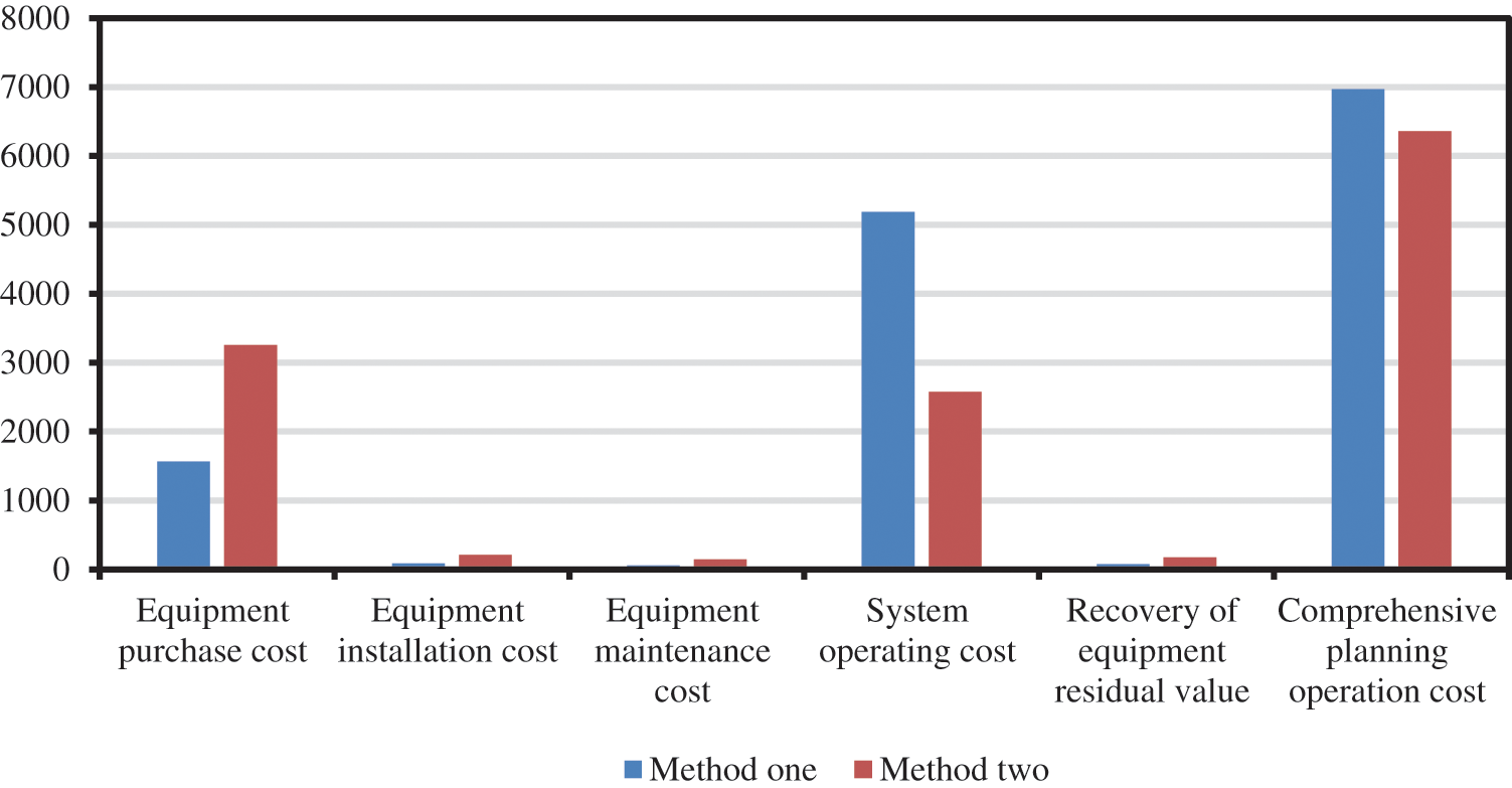
Figure 5: Operating indicators comparison between Mode 1 and Mode 2

It can be seen from Fig. 5 that under the Mode 2, the equipment purchase cost reached 32.5649 million yuan, which was significantly higher than the 15.6355 million yuan under the Mode 1. The higher capacity equipment configuration in the Mode 2 also means higher equipment installation costs, equipment operation and maintenance costs, and equipment residual value recovery. Nevertheless, because the energy interconnected distribution network under the Mode 2 uses multi-energy complementary and coordinated operation to coordinate electricity, heat, and gas, and the coupling of the energy sub-networks has realized the peak shaving and valley filling to a higher degree. Therefore, the operating cost of the system under the whole life cycle has dropped from 51.8703 million yuan in Mode 1 to 25.7569 million yuan in Mode 2. Precisely because of this, the overall planning operating cost of the system has also dropped from 69.6781 million yuan to 63.6023 million yuan, a decrease of 8.72%. At the same time, the system's power supply reliability index has also been increased from 0.994 to 0.997. It can be concluded that under the same scale of energy demands, the operation of the electricity network, thermal energy network and gas network through the energy interconnected distribution network can reduce operating costs and enhance the reliability of the system compared with the independent operation of each energy sub-network.

Take Mode 2 as an example. The convergence of the solution in the first stage determines the optimization of the entire model. The convergence of the algorithm in the first stage of the equipment location and capacity model solution process can be obtained as shown in the figure. It can be seen from Fig. 6 that the solution method of the equipment location and capacity model for energy interconnected distribution network proposed in this paper is suitable for solving this problem.

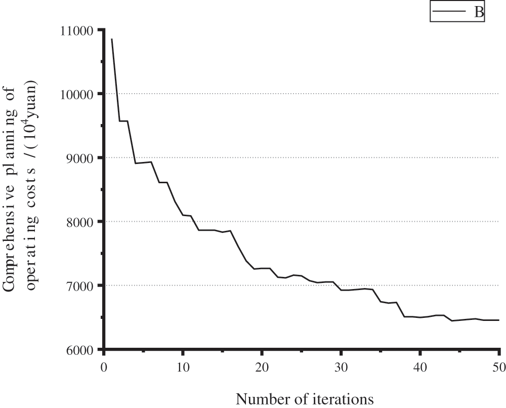
Figure 6: Convergence of the first-stage algorithm under Mode 2

5  Conclusion

In this paper, the location and capacity of equipment in energy interconnected distribution network including electricity network, thermal energy network and natural gas network are deeply studied. Compared with the traditional active distribution network, the proposed model realizes the multi energy complementary and coordinated operation, and significantly reduces the comprehensive operation cost of the system. The specific research results are presented as follows:

(1)   Based on the equipment location and capacity model proposed in this paper, IEEE33 node distribution network system is selected for example analysis. The results show that the multi-energy complementary and coordinated network can have better economic benefits by reducing the comprehensive planning and operation cost of the system.

(2)   Based on the two-stage optimization theory, the high-dimensional problem in the equipment location and capacity model of energy interconnected distribution network proposed in this paper is solved by using binary particle swarm optimization algorithm and chaotic particle swarm optimization algorithm. Compared with the traditional active distribution network model, the effectiveness of the proposed model is verified.

In addition, combined with the current research results and various types of equipment vigorously developed in today's society, it is necessary to further consider the location and capacity of distribution network equipment with multi energy coupling interconnection, which can effectively alleviate the problem of wind and photovoltaic power curtailment, and will also be an important research direction in the future.

Acknowledgement: The completion of this paper has been helped by many teachers and classmates. We would like to express our gratitude to them for their help and guidance.

Funding Statement: The authors received specific funding for State Grid Corporation Headquarters Project Support, Key Technologies and Applications of Planning and Decision-Making Based on the Full Cost Chain of the Power Grid, Grant No. 5205331800001.

Conflicts of Interest: The authors declare that they have no conflicts of interest to report regarding the present study.

References

 1.  Dong, C. Y., Zhao, J. H., Wen, F. S., Xue, Y. S. (2014). From smart grid to energy internet: Basic concept and research framework. Automation of Electric Power Systems, 38(15), 1–11. DOI 10.7500/AEPS20140613007. [Google Scholar] [CrossRef]

 2.  Zhou, H. M., Liu, G. Y., Liu, C. Q. (2014). Study on the energy internet technology framework. Electric Power, 47(11), 140–145. DOI 10.13941/j.cnki.21-1469/tk.2018.11.019. [Google Scholar] [CrossRef]

 3.  Tan, Z. F., De, G., Li, M. L., Lin, H. Y., Yang, S. B. et al. (2019). Combined electricity-heat-cooling-gas load forecasting model for integrated energy system based on multi-task learning and least square support vector machine. Journal of Cleaner Production, 248(14), 119252. DOI 10.1016/j.jclepro.2019.119252. [Google Scholar] [CrossRef]

 4.  Jiang, H. Z., Zhang, C. Y. (2021). Research on location and capacity of distributed units considering renewable energy. Renewable Energy Resources, 39(9), 1248–1254. DOI 10.3969/j.issn.1671-5292.2021.09.016. [Google Scholar] [CrossRef]

 5.  Venkatesan, C., Kannadasan, R., Alsharif, M. H., Kim, M. K., Nebhen, J. (2021). A novel multiobjective hybrid technique for siting and sizing of distributed generation and capacitor banks in radial distribution systems. Sustainability, 13(6), 3308. DOI 10.3390/su13063308. [Google Scholar] [CrossRef]

 6.  Liang, Z. B., Gao, S., Wang, Q., Du, P., Dai, Y. et al. (2021). Multi-objective planning and solution for location and capacity of high-permeability wind power generation based on game strategy. Electrotechnical, 15(1), 1–4. DOI 10.19768/j.cnki.dgjs.2021.15.001. [Google Scholar] [CrossRef]

 7.  Su, L., Dong, X. Y., Zhang, S., Wang, H. Y., Guo, J. (2021). Research on location and capacity of distributed power supply based on multi-objective planning. Automation and Instrumentation, 5(259), 138–141. DOI 10.14016/j.cnki.1001-9227.2021.05.138. [Google Scholar] [CrossRef]

 8.  Habib, F., Asadi, E., Sadjadi, S. J., Barzinpour, F. (2017). A multi-objective robust optimization model for site-selection and capacity allocation of municipal solid waste facilities: A case study in Tehran. Journal of Cleaner Production, 11(166), 816–834. DOI 10.1016/j.jclepro.2017.08.063. [Google Scholar] [CrossRef]

 9.  Wang, Y. L., Wang, J. Y., Gao, M. C., Zhang, D. Y., Liu, Y. et al. (2021). Cost-based siting and sizing of energy stations and pipeline networks in integrated energy system. Energy Conversion and Management, 5(235), 113958. DOI 10.1016/j.enconman.2021.113958. [Google Scholar] [CrossRef]

10. Gao, J. W., Men, H. J., Guo, F. J., Liu, H. H., Li X, Z. et al. (2021). A multi-criteria decision-making framework for compressed air energy storage power site selection based on the probabilistic language term sets and regret theory. The Journal of Energy Storage, 37(3), 102473. DOI 10.1016/j.est.2021.102473. [Google Scholar] [CrossRef]

11. Mortaz, E., Vinel, A., Dvorkin, Y. (2019). An optimization model for siting and sizing of vehicle-to-gird facilities in a microgrid. Applied Energy, 242, 1649–1660. DOI 10.1016/j.apenergy.2019.03.131. [Google Scholar] [CrossRef]

12. Meng, S., Han, Z. X., Sun, J. W., Xiao, C. S., Zhang, S. L. et al. (2020). A review of multi-criteria decision making applications for renewable energy site selection. Renewable Energy, 157, 377–403. DOI 10.1016/j.renene.2020.04.137. [Google Scholar] [CrossRef]

13. Carrión, J. A., Estrella, A. E., Dols, F. A., Toro, M. Z., Rodríguez, M. et al. (2008). Environmental decision-support systems for evaluating the carrying capacity of land areas: Optimal site selection for grid-connected photovoltaic power plants. Renewable and Sustainable Energy Reviews, 12(9), 2358–2380. DOI 10.1016/j.rser.2007.06.011. [Google Scholar] [CrossRef]

14. Nojavan, S., Mohammadi-Ivatloo, B., Zare, K. (2015). Optimal bidding strategy of electricity retailers using robust optimisation approach considering time-of-use rate demand response programs under market price uncertainties. Generation Transmission & Distribution IET, 9(4), 328–338. DOI 10.1049/iet-gtd.2014.0548. [Google Scholar] [CrossRef]

15. Cetinay, H., Kuipers, F. A., Guven, A. N. (2017). Optimal siting and sizing of wind farms. Renewable Energy, 2(101), 51–58. DOI 10.1016/j.renene.2016.08.008. [Google Scholar] [CrossRef]

16. Su, H. F., Hu, M. J., Liang, Z. R. (2016). Distributed generation & energy storage planning based on timing characteristics. Electric Power Automation Equipment, 36(6), 56–63. DOI 10.16081/j.issn.1006-6047.2016.06.009. [Google Scholar] [CrossRef]

17. Sun, Q. Y., Wang, B. Y., Huang, B. N., Ma, A. Z. (2015). The optimization control and implementation for the special energy internet. Proceedings of the CSEE, 35(18), 4571–4580. DOI 10.13334/j.0258-8013.pcsee.2015.18.002. [Google Scholar] [CrossRef]

18. Sheng, W. X., Duan, Q., Liang, Y., Meng, X. L., Shi, C. K. (2015). Research of power distribution and application grid structure and equipment for future energy internet. Proceedings of the CSEE, 35(15), 3760–3769. DOI 10.13334/j.0258-8013.pcsee.2015.15.003. [Google Scholar] [CrossRef]

19. Luo, C. L., Sun, H. B., Xu, G. Y. (1997). The application of power flow calculation with PQV node for UPFC. Automation of Electric Power Systems, 21(4), 34–36. DOI 10.1016/j.jclepro.2020.123348. [Google Scholar] [CrossRef]

20. Chu, Z., Dou, X. X., Yu, Q. Y. (2017). Multi scene distribution network reconfiguration considering the randomness of wind power. Power System Protection and Control, 45(1), 132–138. DOI 10.7667/PSPC160035. [Google Scholar] [CrossRef]

21. Zhang, Q. Y., Li, H. L., Liu, Y. L., Ouyang, S. R., Fang, C. T. et al. (2021). A new quantum particle swarm optimization algorithm for controller placement problem in software-defined networking. Computers & Electrical Engineering, 10(95), 107456. DOI 10.1016/j.compeleceng.2021.107456. [Google Scholar] [CrossRef]

22. Yang, J. Y., Cui, J., Tian, Y. F., Li, L. F., Xing, Z. X. (2015). Multi-objective optimization strategy for distribution network containing dispersed wind farm considering minimum network loss. Power System Technology, 39(8), 2141–2147. DOI 10.13335/j.1000-3673.pst.2015.08.012. [Google Scholar] [CrossRef]

23. Zhang, Y. Z., Zhang, X. P., Lan, L. H. (2022). Robust optimization-based dynamic power generation mix evolution under the carbon-neutral target. Resources, Conservation and Recycling, 178, 106103. DOI 10.1016/j.resconrec.2021.106103. [Google Scholar] [CrossRef]

This work is licensed under a Creative Commons Attribution 4.0 International License, which permits unrestricted use, distribution, and reproduction in any medium, provided the original work is properly cited.