Energy Engineering

DOI: 10.32604/ee.2022.018411

ARTICLE

A STA Current-Constrained Control for PMSM Speed Regulation System with Function Disturbance Observer

Bin Zhang and Boqiang Wei*

Lanzhou Jiaotong University, Lanzhou, 730070, China
*Corresponding Author: Boqiang Wei. Email: 13919943106@163.com
Received: 23 July 2021; Accepted: 01 November 2021

1  Introduction

Permanent magnet synchronous motor (PMSM) is widely used in various high-precision servo systems because of its small size, relatively simple structure, strong reliability, and flexible control. In the non-cascade control structure, PI control can not overcome the problem of excessive starting current, and the control effect will be reduced when the parameters change and external disturbance, which can not meet the requirements of high-performance speed control. Therefore, the design of composite controller with overcurrent protection, ensuring the rapidity, and robustness of the system and analyzing and compensating the disturbance has become a research hotspot.

Up to now, in the framework of field-oriented control (FOC), the cascade structure composed of the current inner loop and speed outer loop is widely used in permanent magnet synchronous motor control systems. In the past, due to computer computing power and memory limitations, the control period of the speed loop in the permanent magnet synchronous motor speed control system was longer than the current loop (usually 5 to 10 times that of the current loop). With the development of computer technology, in recent years, the control cycle of the speed loop and current loop is gradually converging, and the same cycle control should be achieved [1]. Therefore, in some application scenarios, the current loop and speed loop should be combined to form a non-cascade structure. Compared with the cascade structure, the non-cascade structure is easier to implement and uses fewer adjustable parameters. This structure has attracted more and more attention in recent years. For example, in reference [2], an adaptive fuzzy controller combined with a neural network is used to deal with nonlinear friction torque, which uses a single loop structure to reduce the complexity. In reference [3], to avoid excessive overshoot and oscillation, the bandwidth of cascade linear control is limited. In order to overcome the limitation of cascade linear control, a single loop control model predictive direct speed control (MP-DSC) is proposed. In reference [4], a continuous nonsingular terminal sliding mode control method with a non-cascade structure is proposed for mismatched disturbance systems.

However, the non-cascade structure has the advantages of a simple structure, but it still has the critical problem of over-current protection [5]. The non-cascade structure combines the speed loop and the current loop into one so that the q-axis current is changed from the original current loop output to a state of the PMSM control system. Therefore, the traditional PID control of PMSM can not guarantee that the q-axis current is limited within the allowable range. In practical application, excessive instantaneous current will cause hardware damage. In order to solve this problem, we usually choose more conservative control parameters, which sacrifice the dynamic characteristics of the motor control system to a certain extent.

Therefore, the design of state constrained controller is challenging both in theory and practice. At present, several control methods are proposed for state-constrained control. Kosut proposed invariant set, characterized by the fact that the state starting from the invariant set will always remain in the invariant set [6]. Vassilaki et al. [7] constructed a Lyapunov function to generate the largest positive invariant set contained in the constraint domain. However, the estimation of the invariant set depends on the Lyapunov function, and the approximate process needs a lot of calculation. Wills et al. [8] proposed to use Model Predictive Control (MPC) to deal with constraint problems. The principle of MPC is to transform control design problems into optimization problems. By properly selecting the weights of the constrained states, the state constraints are introduced into the cost function. Won et al. [9] considered MPC is used to deal with both current constraints and voltage constraints. Zhang et al. [10] proposed a new FCS-MPC strategy based on fast vector selection, which reduces the amount of calculation in the control process while improving the robustness and control accuracy of the system. Cimini et al. [11] designed an EMPC voltage controller based on a brushless DC motor and carried out a complete physical verification on the DSP. Du et al. [12,13] designed a nonlinear model predictive controller for the constraint management of aero-engines to realize the constraint management of the engine output. However, there are still some shortcomings in the use of MPC. Firstly, MPC needs accurate system modeling, and it is difficult to deal with disturbances. Secondly, it has a large amount of calculation, which brings difficulties to the design. Recently, the improved backstepping method has attracted significant attention [14]. The improved backstepping method provides a scheme for constraint control, but the backstepping method itself still has limitations. The state constraints need to be transferred to the virtual controller to make the parameters more conservative in the design process.

According to the above analysis, to realize the current constraint control of the single-loop structure of the PMSM system, the following conditions need to be met: (1) the current constraint is realized; (2) the control algorithm is easy to implement; (3) it has a good dynamic and steady-state. The design of a new type of current constraint controller in this paper is different from previous studies. The design of this paper does not need to limit the initial conditions (such as invariant sets), and it also avoids a large amount of calculation (such as MPC) or the use of other constraint processing tools (such as Cost function or barrier Lyapunov function).

The new current constrained controller combines the current loop and speed loop control into one controller, sets the given current as a state variable, and adds a penalty term in the controller gain to constrain the q-axis current. The robustness is not strong because the conventional PI control is vulnerable to parameter changes and external disturbance [14]. In order to solve this problem, scholars at home and abroad have researched in related fields and proposed various control methods, which have been successfully applied to the PMSM control system. Among them, sliding mode control (SMC) has become a research hotspot because of its strong robustness to system parameter perturbation and external disturbance, a small amount of calculation, simple implementation, and fast dynamic response, and has been widely used in PMSM speed control systems. But when the sliding mode variable structure control is applied to the actual motor control system, large chattering will make the torque ripple more intense, reduce the stability of the system, and is not conducive to the effective operation of the motor system. Therefore, reducing chattering becomes the critical goal of sliding mode control.

In order to reduce the effect of chattering as much as possible, Hou et al. [15] used saturation or continuous function to replace the saturation function in the reaching law, which can reduce the chattering without reducing the reaching speed. However, this method weakens the robustness of sliding mode control. Asad et al. [16] proposed a variable-speed approaching law based on an inverse hyperbolic sine function, which significantly reduces the buffeting of the system in the steady-state. However, the approaching law has too slow approaching speed, and it has not been applied to the actual system. Zhang et al. [17] proposed a special second-order sliding mode superdistortion algorithm (STA), which makes the system robust and eliminates the output control signal chattering. Therefore, the algorithm is widely used in the motor speed control systems. In order to realize the high-order sliding mode algorithm, a second-order sliding mode algorithm with sliding mode variables is required. The algorithm implementation does not require the derivative of the sliding mode variable, so the control systerm structure is simplified. Su et al. [18] described a direct power control method for designing a doubly-fed asynchronous generator based on the super-twist algorithm, which effectively handles the external disturbance of the system, the existence of model uncertainty, and the nonlinear behavior of the system. Sun et al. [19,20] used STA in the design of the position controller of the permanent magnet planar motor and the torque and flux linkage controller of the induction motor, but this method does not simultaneously perform the second-order sliding mode control on the inner and outer loops of the control system. Wang et al. [21] constructed a fast STA algorithm by adding the proportional term of the sliding mode variable to the STA and applied the algorithm to the outer speed loop, which shortened the system response time again. However, this method ignores the influence of the disturbance term in the control law on the control performance of the system.

Disturbance has a significant influence on the system because the disturbance value can not be measured directly in the existing system, so the design of disturbance observer becomes a necessary step. It is found that the traditional frequency-domain multi-objective observer using unity-gain low-pass filter can only effectively deal with a class of specific disturbances satisfying the so-called matching conditions. In contrast the traditional time-domain multi-objective observer always produces high-order observers. For this reason, a functional interference observer (FDOB) is proposed to improve the existing results and design criteria, frequency analysis, and existence conditions [22]. Compared with the existing frequency-domain disturbance observer, the proposed functional disturbance observer (FDOB) can handle more kinds of disturbances, while compared with the existing time-domain disturbance observer, the proposed functional disturbance observer (FDOB) can produce a lower order observer.

Therefore, this paper proposes to combine current restraint control and super-twist control in a non-cascade structure to produce a super-twisted current restraint controller (CCSTA). At the same time, in order to improve the anti-interference ability of the system, FDOB is used for compensation. A composite controller is composed of CCSTA and FDOB. The composite controller can constrain the q-axis current of PMSM to reduce the starting current and prevent the equipment from being damaged by excessive current. At the same time, Super Twisted Sliding Mode Control (STA) ensures the robustness and rapidity of the system. The matched and unmatched disturbances are observed and compensated through the Constructed Function Disturbance Observer (FDOB), which further improves the system's response efficiency and anti-disturbance performance.

2  Mathematical Model of PMSM

Assuming that the magnetic circuit is unsaturated, ignoring hysteresis and eddy current losses, the magnetic field is distributed in a sinusoidal space. Under this condition, the mathematical model of the attached permanent magnet synchronous motor in the coordinate system should be described as

(id∙i∙qω∙)=(−RSLnpω0−npω−RSL−npψfL0npψfJ−BJ)(idiqω)+(udLuqL−TLJ)(1)

where udand uq are the stator voltages of d-axis and q-axis, idand iq are the stator currents of d-axis and q-axis, ω is the angular velocity, np is the pole number, L is the stator inductance, RS is the stator resistance, ψf is the rotor flux, TL is the load torque, J is the moment of inertia, B is the viscous friction coefficient.

Considering the variation of system parameters and load torque, the motion equation of PMSM rotor should be expressed as

dωdt=−(BJ+Δa)ω−(TLJ+Δc)+(npψfJ−Δb)iq=aω+bu−d(2)

where, a=−BJ,b=npψfJ,u=iq is a control law to be designed Δa,Δb,Δc represents the perturbation of motor parameters, d is the disturbance caused by the change of system parameters and load, and

d=Δaω+Δbu+Δc+TLJ(3)

Considering the current constraint, the q-axis current is limited to |iq|<c, where c is a positive constant.

Hypothesis 1: The load torque variation satisfies the following conditions:

2TL+Bω∗npψf<corTL<npψf(c−iq∗)(4)

where iq∗=TL+Bω∗npψf is the current balance point.

Note 1.1: Hypothesis 1 makes the current constraint still have the margin to suppress the load variation under the condition of load uncertainty, so there must be c -i*q>0. Choosing the value of c according to the rated current of PMSM, which is usually two to three times the rated current. In this paper, c = 15A.

3  Design of Current Constrained Controller for STA

This section studies the speed tracking and current constraints of the permanent magnet synchronous motor control system. The STA second-order sliding mode control has the fast response characteristics and no chattering in the speed curve. At the same time, to ensure that the starting current does not exceed the limit value, the system adopts a simple and effective STA second-order sliding mode control combined with current constrained control.

3.1 Design of STA Second Order Sliding Mode Controller

The general expression of STA is

u=λ|s|0.5sign(s)+∫αsign(s)dt(5)

where: Control parameters α, λ are used to ensure the stability of the system in a limited time and resist the influence of uncertain factors, and α and λ are positive constant, s is the sliding mode variable.

Make x= ω* - ω combining with Eq. (2), obtain the error equation of the speed of the PMSM.

x⋅=ax−bu+d+M(t)(6)

where: M(t)=ω∗⋅−aω∗.

The correlation degree of the speed error state equation shown in Eq. (2) is 1 [13], which meets the requirements of STA for the system. Therefore, the sliding mode surface is selected as:

s=x=ω∗−ω(7)

In combination with Eqs. (6) and (7), it should be obtained that

s⋅=x⋅=as−bu+d+M(t)(8)

In a practical application system, u should be composed of equivalent control law and switching robust control law

u=ueq+usw(9)

Among them, ueq is the equivalent control part of the system, and usw is the switching part. M(t) is an uncertain term when considering the actual system and should be given randomly. Therefore, M(t) = 0 is tentatively determined when calculating the equivalent control law. In combination with Eq. (8), let s⋅=0, the equivalent control part is

ueq=1b(as+d)(10)

usw is the switching part, usw=λ|s|0.5sign(s)+∫αsign(s)dt. Therefore, the STA control law should be obtained as follows:

u=1b(as+d)+λ|s|0.5sign(s)+∫αsign(s)dt=λ|s|0.5sign(s)+∫αsign(s)dt+abs+1bd(11)

Substituting Eq. (11) into Eq. (8) yields

s⋅=as−bu+d+M(t)=−λ′|s|0.5sign(s)−α′∫sign(s)dt+M(t)(12)

where λ′=bλ,α′=bα, in the process of parameter modulation, system parameter b is integrated into control parameters λ′ and α′. In this way, there is no need to pay attention to the exact value of b, just adjust the values of λ and α.

3.2 Current Constraint Function

The key is to add a penalty mechanism to the q-axis current in the control action to meet the current limit.

In this paper, a nonlinear penalty term lc2−iq2 of iq is constructed directly in the controller. The term is added to the control system as a control gain. When iq approaches ±c, the term will approach infinity, forcing the current to adjust in time. In this way, the controller uq should be adjusted in time to limit the current so that the q-axis current is strictly limited in the safe range. As a penalty parameter, l controls the size of the penalty.

3.3 STA Current Constrained Controller

In this paper, a non-cascade structure is adopted to simplify the structure of the system. At the same time, a fundamental problem needs to be solved, that is, the problem of current constraint. Therefore, a current constraints function is added basis on STA control, that is, the CCSTA, which not only ensures the response efficiency of the system but also does not cause sizeable current damage to the system hardware.

The following is the specific design of ud and uq:

ud=kP(id∗−id)+kI∫(id∗−id)ds−Lnqωiq(13)

uq=λ′|s|0.5sign(s)+∫α′sign(s)dt+(ks+lc2−iq2)(−iq+Bω∗npψf)+npψfω∗+Lnpωid(14)

Among them, kP, kI, ks and l are all controller parameters, id∗=0 is the reference signal of id, (13) and (14) do not depend on the exact values of J and TL.

3.4 Stability Analysis

Let uq=uq1+uq2, where

uq1=λ′|s|0.5sign(s)+∫α′sign(s)dt(15)

uq2=(ks+lc2−iq2)(−iq+Bω∗npψf)+npψfω∗+Lnpωid(16)

In order to prove the stability of the system, it is necessary to analyze the construction of the Lyapunov function for Eqs. (13), (15), and (16). Firstly, the parameters used in the two equations are simplified:

eq1=ω∗−ω(17)

eq2=iq∗−iq(18)

ed0=∫0t(id∗−id)(19)

ed1=id∗−id(20)

eq0=∫0t(ω∗−ω)ds−1kIRiq∗−1kI[ks+lc2−(iq∗)2](TLnpψf)(21)

Therefore, the system error equation should be written in the following form:

{e⋅d0=ed1e⋅d1=−RLed1−npωiq−udLe⋅q0=eq1e⋅q1=−BJeq1+npψfJeq2e⋅q2=−npψfLeq1−RLeq2+npωid+RLiq∗+npψfLω∗−uqL.(22)

Let ϕ¯=c+iq∗,ϕ_=−c+iq∗, according to hypothesis 1, and we can get ϕ¯>0,ϕ_<0, then further have

(c2−iq2)=(ϕ¯−eq2)(eq2−ϕ_)(23)

Thus, the proof |iq|<c is equivalent to the proof eq2∈(ϕ_,ϕ¯). For the convenience of discussing the stability of the error system (22), rewrite uq2 as

uq2=[kS+l(1+Π)(ϕ¯−eq2)(eq2−ϕ_)]eq2+npψfω∗+Lnpωid+Riq∗(24)

Among Π=(TLnpψfc−Bω∗−TL)(iq+iq∗c+iq∗), note Π¯=TLnpψfc−Bω∗−TL,Π_=(TLnpψfc−Bω∗−TL)(−c+iq∗c+iq∗). According to hypothesis 1, we can get Π¯∈(0,1),Π_∈(−1,0). If |iq|<c, then Π_<Π<Π¯.

Theorem 2.1: Under assumption 1, the origin of closed-loop systems (22) and (25) are asymptotically stable. If condition iq(0)∈(−c,c) is satisfied (eq2(0)∈(Π_,Π¯)). Then ω will approach ω* in a limited time. At the same time, the q-axis current satisfies the current constraint.

Proof: Denote e=(ed0,ed1,eq0,eq1,eq2) and Ω=R4×(∏_),Π¯). For any given initial value e(0)∈Ω, suppose [0,T) is the maximum time interval that eq2(t)∈(Π_,Π¯),t∈[0,T) satisfies. According to the selection of initial value e(0), the definition of [0,T) is meaningful, and T should be a normal number or T=+∞.

Therefore, to prove that the current constraint is satisfied, we only need to prove T=+∞.

In the interval [0, T), substituting Eq. (13) and Eq. (24) into (22) should be obtained

{e⋅d0=ed1e⋅d1=−1L(kP+R)ed1−kILed0e⋅q0=eq1e⋅q1=−BJeq1+npψfJeq2e⋅q2=−kILeq0−npψf+kPLeq1−1L[R+kS+l(1+Π)(eq2−ϕ_)(ϕ¯−eq2)]eq2(25)

The Lyapunov function is constructed according to Eqs. (15) and (28)

V=ξTPξ+12ed02+L2kIed1+12eqo2+JBeq0eq1+J(npψf+kP)2kIBeq12+Lnpψf2kIBeq22(26)

Among ξ=[|s|0.5sign(s)∫α′sign(s)],P=12[4α+λ2λλ2], and dξdt=[|s|−0.52(−λ′sign(s)−∫α′sign(s)dt+M(t))α′sign(s)].

The vector field of the

The vector field of the error system (25) is continuously differentiable in Ω. Take the derivative of V in the interval [0, T) and get the result (27):

V·=-|s|−0.5ξTQ1ξ+M(t)|s|0.5Q2Tξ+ed0ed1+L2KI(−RLed1−npωiq−udL)+eq0eq1+JB[eq12+(−BJeq1+npψfJeq2)]+J(npψf+kP)kIBeq1(−BJeq1+npψfJeq2)+LnpψfkIBeq2(−npψfkIBeq1−RLeq2+npωid+RLiq∗−npψfLω∗−uqL)(27)

Among Q1=λ′2[2α′+λ′2λ′λ′1],Q2=[2α′+12λ′212λ′], select δ>0, makes |M(t)|≤δ|s|0.5 holds.

And npψf+kPkI>BJ.

Simplify (27) to obtain Eq. (28).

V•≤−|s|−0.5ξTQ3ξ+ed0ed1−kP+RkIed12−ed0ed1+eq0eq1+JB(eq12−BJeq0eq1+npψfJeq0eq2)+J(npψf+kP)kIB(−BJeq12+npψfJeq1eq2)+LnpψfkIB{−kILeq0eq2−npψf+kPLeq1eq2−1L[R+kS+l(1+Π)(ϕ¯−eq2)(eq2−ϕ_)]eq22}≤−|s|−0.5ξTQ3ξ−kP+RkIed12−(npψf+kPkI−JB)eq12−(R+kS)npψfkIBeq22(28)

Among Q3=λ′2[2α′+λ′2−(4α′λ′+λ′)δλ′−δ2λ′−δ21], the vector field of error system (28) is continuously differentiable in Ω. It should be seen from Eq. (28) that V(t)≤V(0),t∈[0,T), note ρ1=2V(0)F0,F0=BJ(npψfkI−JB),F0=BJ(npψfkI−JB),

ρ0=2V(0)+JBρ1. |eq0(t)|≤ρ0,|eq1(t)|≤ρ1,t∈[0,T) should be obtained from Eq. (26).

It is necessary to prove that there are always constants ϕ1=ϕ1(ρ0,ρ1)∈(0,ϕ¯) and ϕ2=ϕ2(ρ0,ρ1) for any initial value e(0)∈Ω. Such that eq2e˙q2(t)≤0, when e(t)∈R2×[−ρ0,ρ0]×[−ρ1,ρ1]×([ϕ1,ϕ¯)∪(ϕ_,ϕ2]),t∈[0,T).

According to the two cases of eq2(0), we discuss them separately.

Case 1: eq2>0, denote ϕ1=max{eq2(0),F0l(1+Π_)+F0ϕ¯}, among F0=[(kIρ0+(npψf+kP)](ϕ¯−ϕ_), if eq2(t) ∈(ϕ1,ϕ¯],t∈[0,T), then

e˙q2≤1L[kIρ0+(npψf+kP)ρ1−l(1+Π_)eq2(ϕ¯−ϕ_)(ϕ¯−eq2)]≤0(29)

Case 2: eq2<0, donote ϕ2=min{eq2(0),F0l(1+Π_)+F0ϕ_}, if eq2(t)∈(ϕ_,ϕ2],t∈[0,T), then

e˙q2≥1L[−kIρ0−(npψf+kP)ρ1−l(1+Π_)eq2(ϕ¯−ϕ_)(eq2−ϕ_)]≥0(30)

For any given initial value e(0)∈Ω, suppose e(t) is the solution of the error system (28) on the interval μ=R2×(−ρ0−1,ρ0+1)×(−ρ1−1,ρ1+1)×(ϕ¯,ϕ_)⊂Ω. It should be deduced from inequality (30) and (31):

e(t)∈R2×[−ρ0,ρ0]×[−ρ1,ρ1]×[ϕ_,ϕ¯]⊂μ,t∈[0,T)(31)

According to the definition of T, T=+∞ is obtained by using the extension theorem of the solution. That is, the current constraint iq∈(−c,c) is always guaranteed. At the same time, inequality (28) is also holds. By using the Barbarshin theorem [18], the equilibrium points of Eqs. (14), (22), and (25) are asymptotically stable.

Finally verified V∙<0, this completes the proof.

According to the above stability proof, the system is stable when the stability condition is satisfied.

4  Design of Disturbance Observer

Because there are both internal parameter disturbances and external load disturbances in the permanent magnet synchronous motor system, the functional disturbance observer (FDOB) can effectively deal with both disturbances.

4.1 Construction of FDOB Transfer Function

Consider a linear time-invariant system with unknown disturbances.

{x∙=Ax+Bu+Ddy=Cx(34)

Among x∈Rn,u∈R,d∈R,y∈R are system status, control input, disturbance, and measurement output.

Combining with PMSM system, Eq. (1) is replaced by Eq. (34), denote a1=npψfJ,a2=RSL,

a3=npψfL,a4=BJ,a5=npω,b1=1L, we can get

x=(ωiqid),u=(0uqud),A=(0a1−a4−a5−a2−a1−a2a50),B=(0b1b1),C=(101),D=(100)

The disturbance is supposed to be generated by the following linear exogenous system:

{ω∙=Sωd=Hω(35)

Among ω∈Rq and (S, H) is known and observable. The initial state of the disturbance system is assumed to be unknown, Eq. (34) should be applied to most disturbances in real control problems.

Definition 3.1: If the matrix in (35) satisfies det (S) = 0, the disturbance is defined as type I disturbance, and if det(S)≠0, the disturbance is defined as type II disturbance.

By combining Eqs. (34) and (35), a composite system should be obtained

{x¯∙=A¯x¯+B¯uy=C¯x¯(36)

Among x¯=[xT,ωT]T, the following is the system matrix:

A¯=(ADHOq×nS),B¯=(BOq×1),C¯=(CO1×q)

For the system (35) with disturbance (34), choosing FDOB as disturbance observe, then the transfer function of disturbance estimation is given by the following formula:

d^(s)=−Gud^(s)u(s)+Gyd^(s)y(s)(37)

Among

Gud^(s)=Hadj(sI−S)J2Mn(s)det(sI−F)(38)

Gyd^(s)=Hadj(sI−S)J2Nn(s)det(sI−F)(39)

Gn(s)=Mn(s)Nn(s)(40)

Gn(s) is the nominal value of the system transfer function.

F=U−ZV(41)

U=LA¯L+−LA^∑+Ψ(42)

V=(I−ΣΣ+)Ψ(43)

Among L=[L000Iq] is the gain matrix of FDOB, L+ is the pseudo inverse of L. A^=A¯(I−L+L), C^=C¯(I−L+L),Σ=[C¯A^C^], ∑+ is the pseudo inverse of ∑.Ψ=[C¯A¯L+C¯L+], Z are any compatible matrix, and [J,K]=[J1K1J2K2]=LA^∑++Z(I−∑∑+).

4.2 The Existence Condition of FDOB

FDOB can significantly reduce the order of disturbance observer, but the existing condition of FDOB should be satisfied when choosing the gain L. According to [22], the existing condition of FDOB is that F satisfies the Hurwitz theorem:

rank([sL−LA¯C¯A¯C¯])=rank([C¯A¯C¯L]),∀s∈C,Re(s)≥0(44)

4.3 The Difference between FDOB and Frequency Domain DOB

According to the literature [22], it should be obtained that the existing frequency-domain DOBs are subject to considerable restrictions in their use. Gud^(0)=1 (disturbance matching) should be realized only when the two conditions of D = B and det(S) = 0 are met simultaneously. This means that the frequency domain DOB using the low-pass filter Q (s) with unit DC gain can only effectively deal with matched type I interference, not general interference or mismatched interference. The FDOB part of the system status should be obtained directly from the measured value y=C¯x¯. where C¯ is the measurement matrix and x¯ is the system state matrix. Therefore, there is no need to estimate this part of the state, and sometimes even a part of the unmeasurable state does not need to be estimated for the purpose of interference estimation. So FDOB has broader practicability than frequency-domain DOB [23–25].

5  Composite Control Design

Under the condition of meeting the current constraint, the disturbance observation should be realized at the same time. The compound control design of super twisting current constraint control and functional disturbance observer compensation is adopted. The following is the composite control law [26,27].

{ud=kP(id∗−id)+kI∫(id∗−id)ds−Lnqωiquq=λ|s|0.5sign(s)+∫αsign(s)dt+(ks+lc2−iq2)(−iq+Bω∗npψf)+npψfω∗+Lnpωid+d^(45)

The non-cascade structure of the composite controller is shown in Fig. 1.

Figure 1: The principle block diagram of PMSM system based on STA current constraint controller

6  Simulation Research and Analysis

In order to verify the effectiveness of CCSTA + FDOB composite controller. The simulation model is established based on MATLAB/Simulink platform. The parameters of PMSM in the simulation are shown in Table 1.

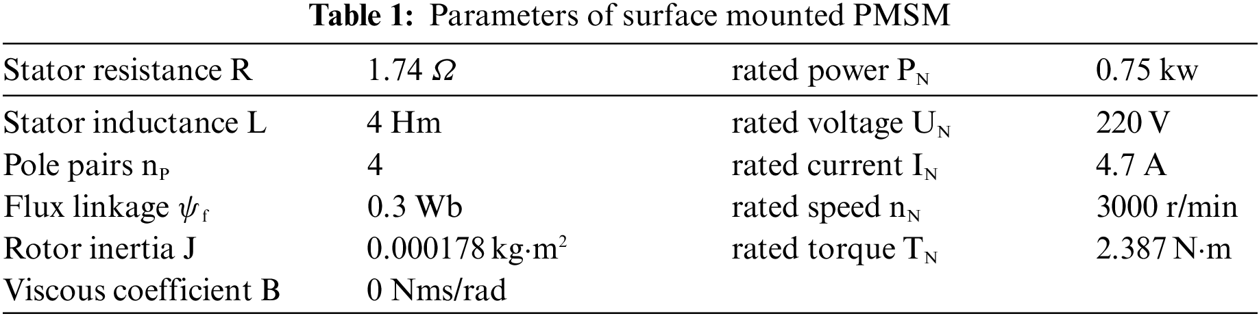
In this paper, a composite controller combining current constrained sta with functional disturbance observer is designed. Its parameter configuration are l = 1, λ=3.3, α=100, ks = 0.3, KP = 230, KI = 10, The pole assignment of FDOB are p1=−30, p2=−40, p3=−50.

In order to verify the functions of the control system proposed in this paper in terms of current constraints and anti-disturbance functions, the following comparison will be made. First, compare CCSTA with STA to verify the current restraint ability of CCSTA. Parameter configuration of STA controller: speed loop k1 = 1, k2 = 80, current loop k1 = 30, k2 = 500.

It should be seen from Fig. 2 that the current restraint function of CCSTA makes the starting current be restrained within a limited range, while the current of STA without the current restraint function exceeds the limited range.

Figure 2: Current constraint comparison

Compare CCSTA + FDOB with CCSTA + DOB to verify the anti-disturbance ability of FDOB. The DOB parameter configuration is α1 = 15, α2 = 9, and ε = 0.005.

It should be seen from Fig. 3 that when the step disturbance action is used in the system, the response time of CCSTA + FDOB is 0.001 s with a speed change of 12 r/min, and the response time of CCSTA + DOB is 0.006 s with a speed change of 60 r/min. Therefore, FDOB has better performance when dealing with matching step disturbances. Fig. 4 shows the performance of the two methods under mismatched sinusoidal disturbances.

Figure 3: Step disturbance comparison

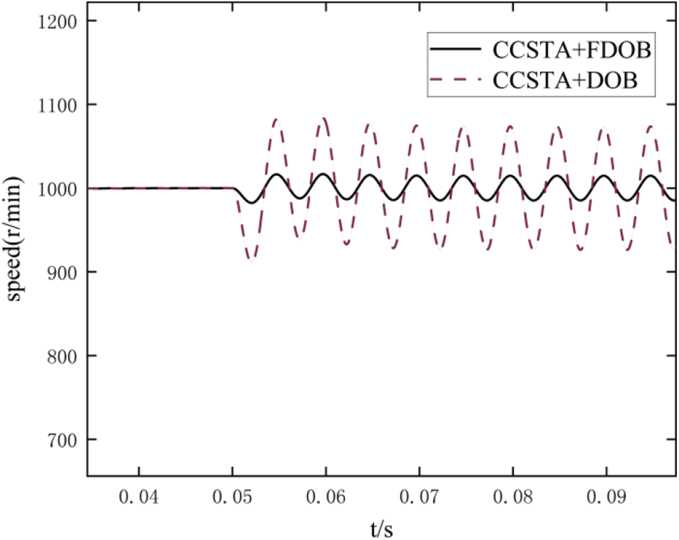
Figure 4: Mismatched sinusoidal perturbation comparison

The impact of CCSTA + FDOB is significantly less than that of CCSTA + DOB, so FDOB has better anti-interference performance against sinusoidal disturbances. The model predictive control (MPC) is compared with the super twisted current restraint control (CCSTA) to verify the progressive nature of the current restraint ability of CCSTA.

The cost function J of MPC is defined as,

J=kαCω+kβCc+kχCl(46)

Cω=|ωr∗(k)−ωr(k+2)|+|ωr∗(k)−ωr(k+2)|(47)

Cc=|id∗(k)−id(k+2)|+|iq∗(k)−iq(k+2)|(48)

Cl={∞,|is(k+2)|>imax0,|is(k+2)|≤imax(49)

It should be seen from Fig. 5 that the CCSTA response time is 0.004 s, the overshoot is 0.5%, the MPC response time is 0.006 s, and the overshoot is 0%. It should be seen from Fig. 6 that both MPC and CCSTA limit the current within the limit range, but the q-axis starting current of MPC is close to the limit value. In contrast, the current constraint ability of CCSTA makes the system safer, and the structure of CCSTA is simpler than that of MPC.

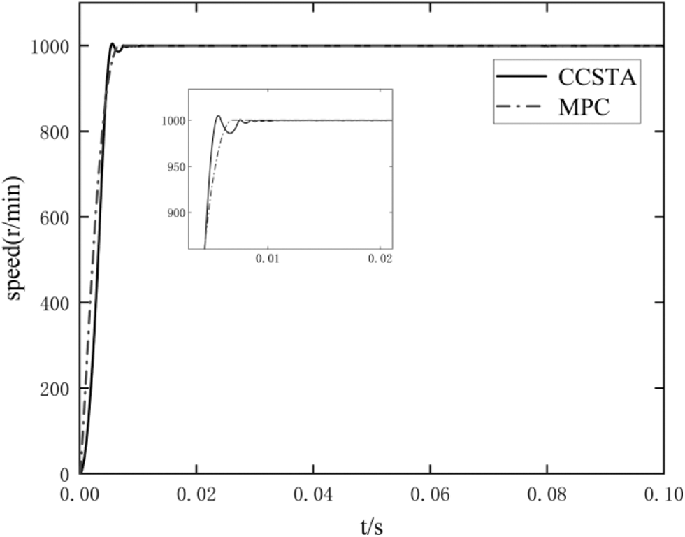
Figure 5: Comparison of motor starting speed response

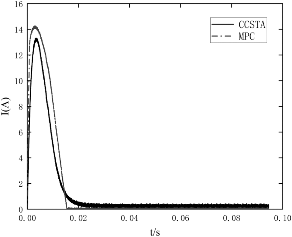
Figure 6: Comparison of q-axis starting current response

In order to verify the performance of the control method proposed in this paper, the composite controller combining the Super Twist Controller (STA) and the Disturbance Observer (DOB), and the composite controller combining the PD controller and the Extended State Observer (ESO) are compared. The parameter configuration of STA and DOB composite controller is as follows: Speed loop k1 = 1, k2 = 80, current loop k1 = 30, k2 = 500, disturbance observer α1 = 15, α2 = 9, ε = 0.005. The parameter configuration of PD and ESO composite controller is as follows: Speed loop kp1 = 11, kd1 = 0.04, current loop kp2 = 30, ki2 = 500, ESO β01 = 7810, β02 = 640, α = 0.5, δ = 0.01. It is assumed that CCSTA + FDOB composite control system is scheme 1 and STA + DOB composite control system is scheme 2, PD + DOB is scheme 3.

Figs. 8–10 show the speed, current, and voltage response curves of the three control schemes of PMSM at the start-up stage. It should be concluded from Fig. 8 and Table 2 that scheme 1 has the shortest response time and the smallest overshoot, and the CCSTA + FDOB composite control system can effectively improve the dynamic performance of the system. It should be seen from Figs. 9 and 10 that the current constraint in scheme 1 effectively controls the current within the limit value and does not cause adverse effects on the system rapidity and stability, while scheme 2 and scheme 3 fail to limit the current within the limit value.

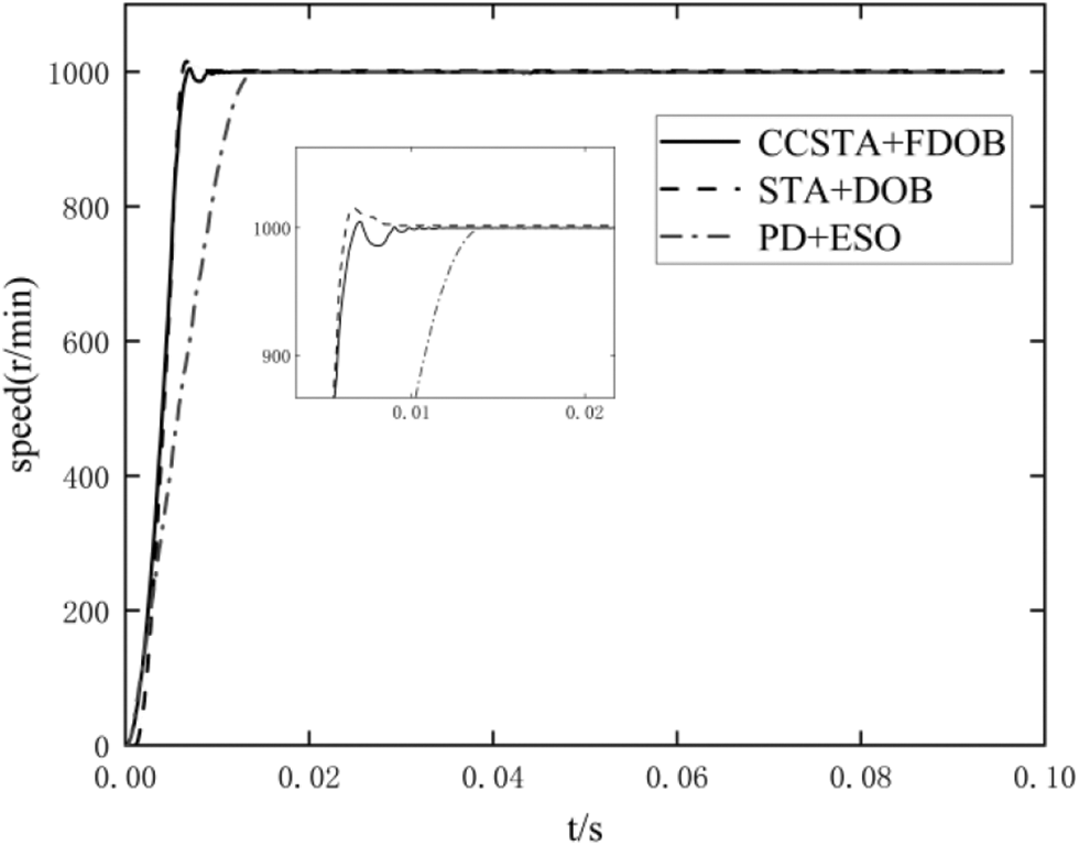
Figure 8: Speed response comparison of motor under no load starting

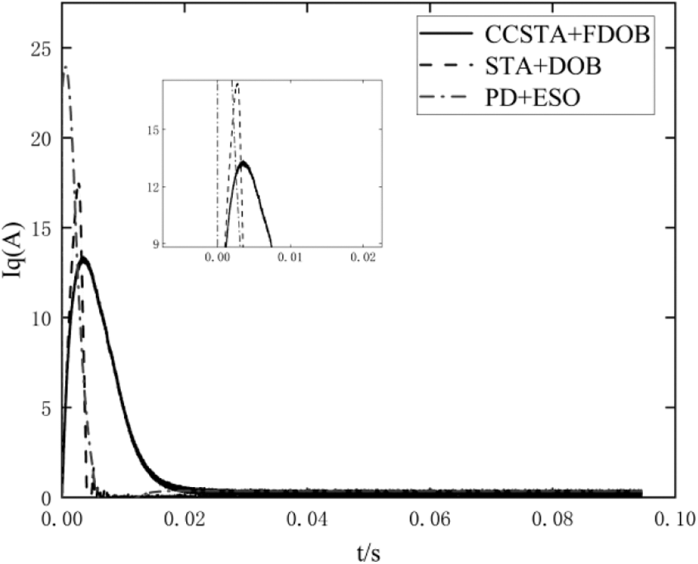
Figure 9: q-axis current response curve

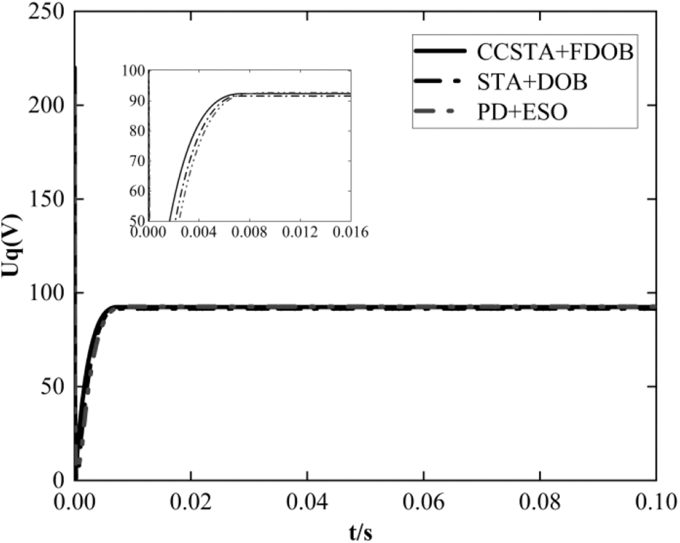
Figure 10: Q-axis voltage response curve

Figs. 11–13 show the steady-state torque curves of the three schemes when the system is given 5 N ⋅ m load torque. Fig. 5 shows the steady-state torque curve of the PD + ESO composite controller, with a ripple range of 4∼6.1 N⋅m, the torque ripple is 42%. Fig. 6 is the steady-state torque curve of STA + DOB composite controller, with a torque ripple range of 4.1∼5.5 N⋅m and torque ripple of 28%. Fig. 7 shows the steady-state torque curve of the CCSTA + FDOB composite controller, with torque ripple range of 4.9∼5.1 N⋅m and a torque ripple of 4%. It should be seen that the current constrained STA composite controller can further suppress the torque ripple.

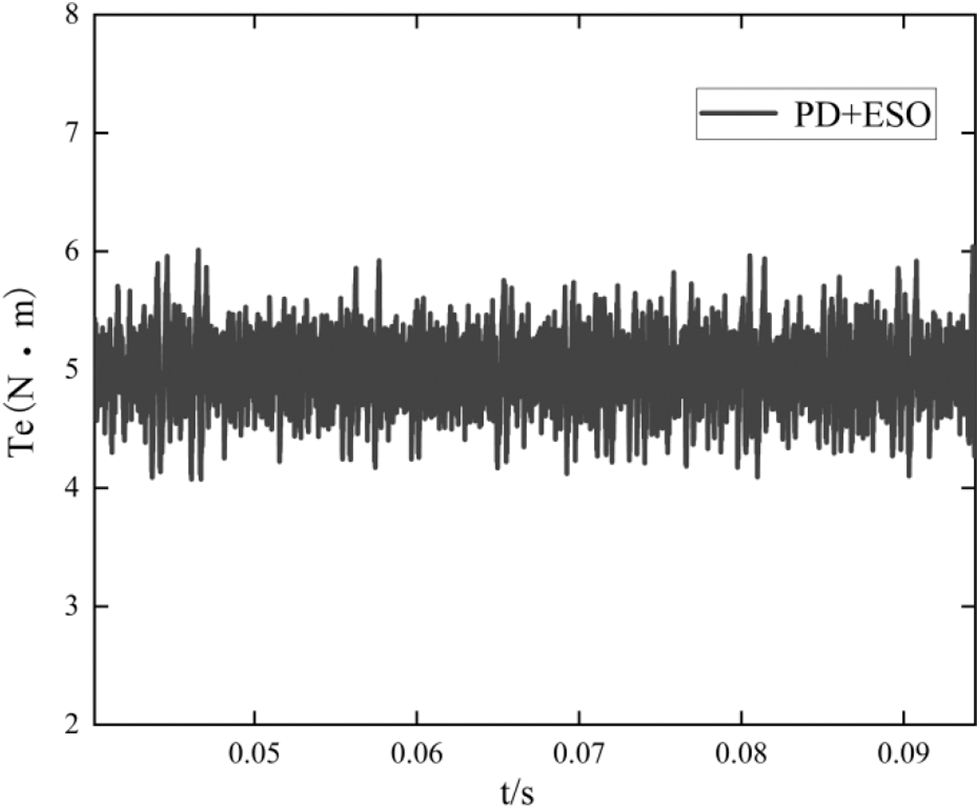
Figure 11: Steady state torque curve of PD + ESO

Figure 12: Steady state torque curve of STA + DOB

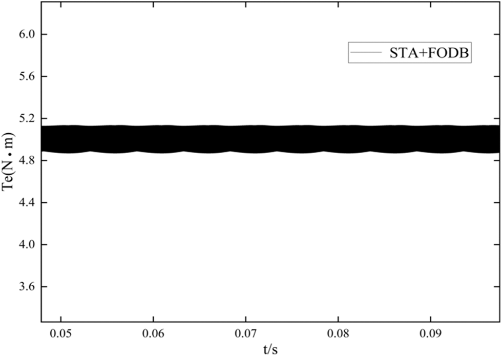
Figure 13: Steady state torque curve of CCSTA + FDOB

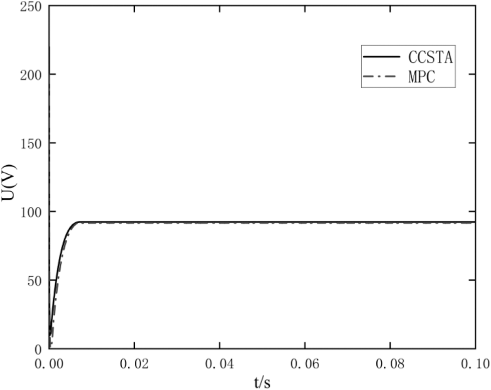
Figure 7: Comparison of q-axis starting voltage response

In order to test the performance of the proposed composite system in the case of up and down speed, the simulation results show that the expected speed at the initial time is 200 r/min, the expected speed is increased to 1000 r/min at 0.02 s, and the expected speed is reduced to 500 r/min at 0.06 s. The system runs under the load of 3 N⋅m.

It should be seen from Fig. 14, Tables 3 and 4 that the composite controller designed in this paper has the shortest response time and the lowest overshoot in the process of variable speed regulation, which ensures the stability of the system in the process of variable speed regulation. The overshoot and response time of the other two schemes are too large in the process of variable speed, which negatively affects on the system speed stability.

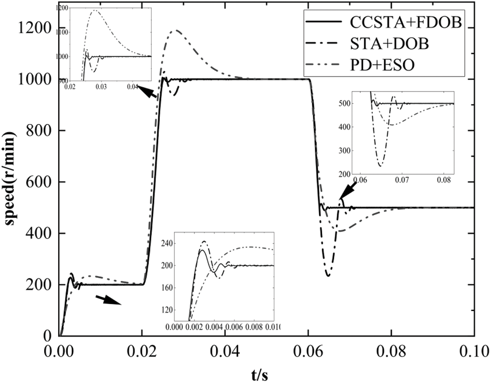
Figure 14: System variable speed response curve

In this design, FDOB has the function of estimating and compensating mismatched disturbance. Suppose the system has an unknown mismatched step disturbance. Let S = 0, H = 5, L0 = [0 1] the unknown step disturbance acts on the system at 0.04 s.

It should be seen from Fig. 15 that the response time of scheme 1 is 0.001 s when the step disturbance acts on the system, with a speed change of 12 r/min, the response time of scheme 2 is 0.007 s with a speed change of 100 r/min, and that of scheme 3 is 0.014 s with a speed change of 140 r/min. Among the three schemes, scheme 1 has the shortest response time and the slightest speed change. Therefore, the system designed in this paper has better anti-disturbance ability in unknown step disturbance.

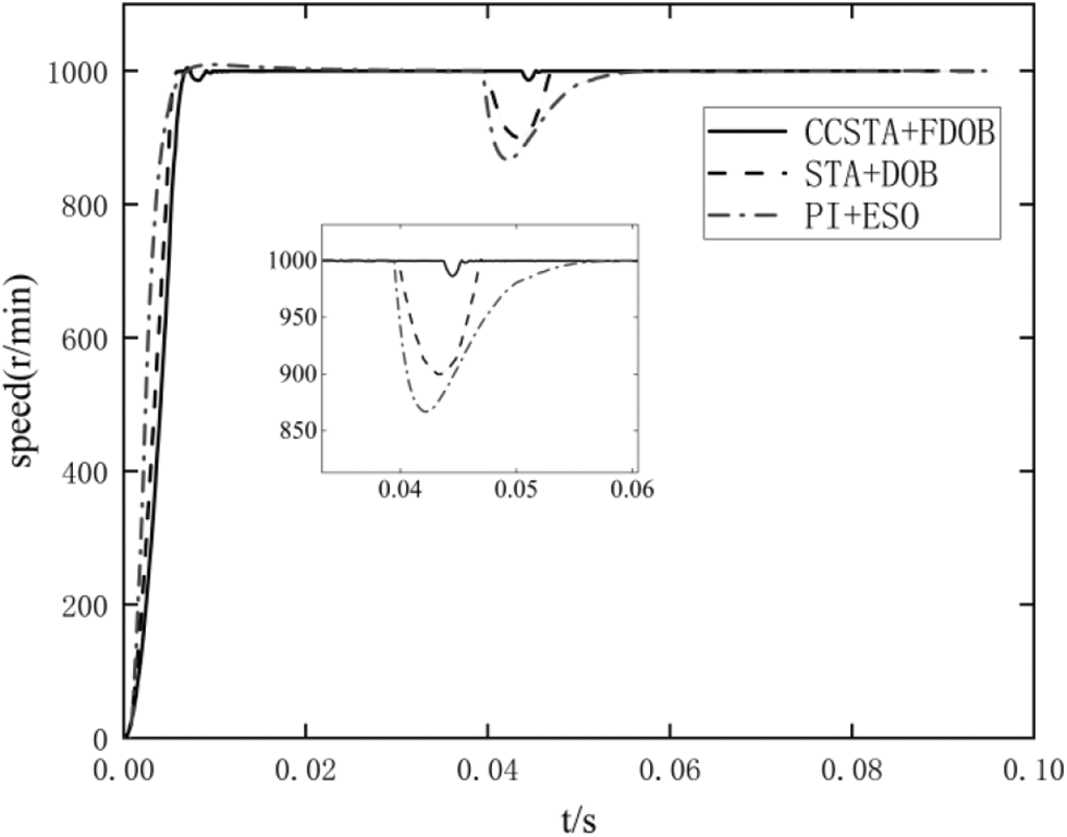
Figure 15: Mismatched step disturbance

It is assumed that a sinusoidal disturbance with known frequency and unknown amplitude and phase is used in the system. Let S = [62800−628], H = [1 0], matrix L0 be selected as L0 = [0 1], and the sine wave perturbation acts on the system in 0.05 s.

It should be seen from Fig. 16 that under sinusoidal disturbance, the influence of the composite controller designed in this paper is obviously less than that of the other two schemes, and FDOB has good following and anti disturbance performance to sinusoidal disturbance.

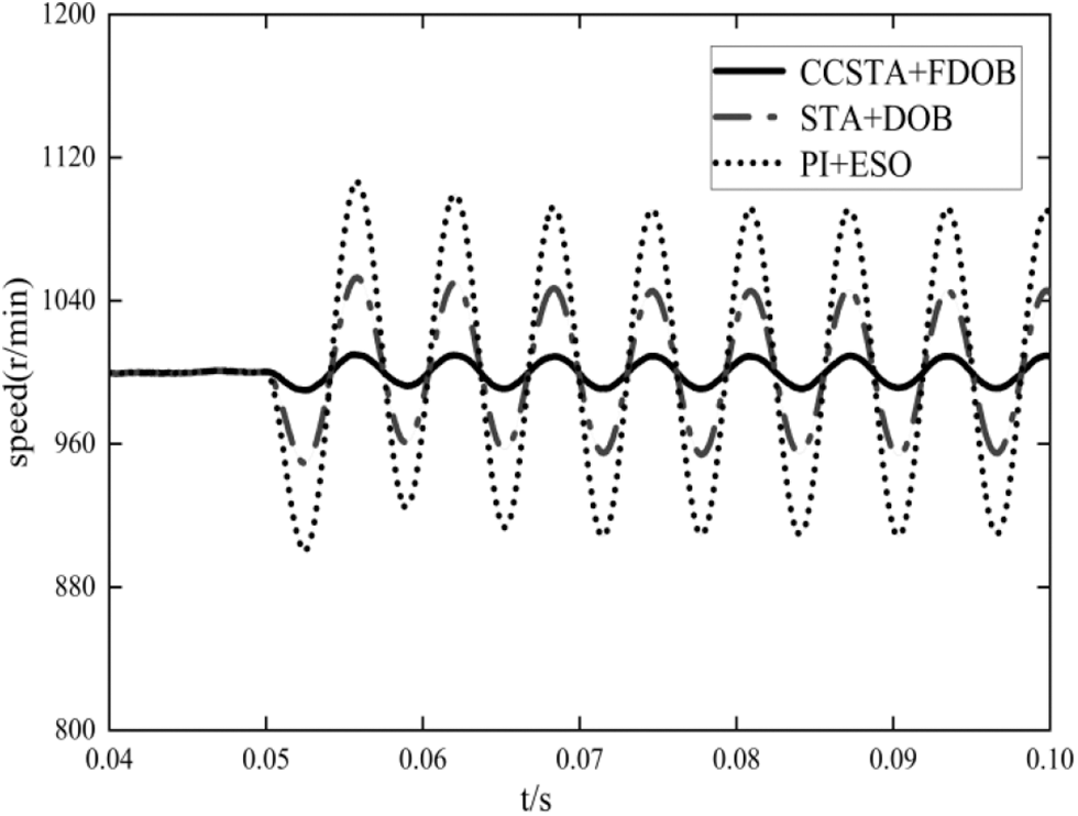
Figure 16: Sine wave disturbance

7  Conclusion

This paper combines current constrained control and super twist second-order sliding mode control (STA). At the same time, the super twist sliding mode control (STA) can effectively reduce the system response time and suppress the steady-state chattering. In order to avoid the influence of internal and external disturbance on the system, the function disturbance observer (FDOB) is designed to compensate for the system disturbance. FDOB can estimate and compensate the system matching and mismatching disturbance, improve the system's anti disturbance performance, and verify the system function through comparison. In this paper, three control strategies of the CCSTA + FDOB control system combined with STA + DOB control system and PD + ESO control system are simulated and compared. The results verify the feasibility and effectiveness of the proposed control algorithm.

Funding Statement: This work was supported by the National Natural Science Foundation of China under Grant 61863023.

Conflicts of Interest: The authors declare that they have no conflicts of interest to report regarding the present study.

Reference

 1.  Sun, Z., Guo, T., Wang, X., Yan, Y., Li, S. (2017). A composite current constrained control for PMSM with time-varying disturbance. Advances in Mechanical Engineering, 9(9), 1–13. DOI 10.1177/1687814017728691. [Google Scholar] [CrossRef]

 2.  Chaoui, H., Sicard, P. (2013). Adaptive fuzzy logic control of permanent magnet synchronous machines with nonlinear friction. IEEE Transactions on Industrial Electronics, 59(2), 1123–1133. DOI 10.1109/TIE.2011.2148678. [Google Scholar] [CrossRef]

 3.  Preindl, M., Bolognani, S. (2013). Model predictive direct speed control with finite control set of PMSM drive systems. IEEE Transactions on Power Electronics, 28(2), 1007–1015. DOI 10.1109/TPEL.2012.2204277. [Google Scholar] [CrossRef]

 4.  Yang, J., Li, S., Su, J., Yu, X. (2013). Continuous nonsingularterminal sliding mode control for systems with mismatched disturbances. Automatica, 49(7), 2287–2291. DOI 10.1016/j.automatica.2013.03.026. [Google Scholar] [CrossRef]

 5.  Bolognani, S., Bolognani, S., Peretti, L., Mauro, Z. (2009). Design and implementation of model predictive control for electrical motor drives. IEEE Transactions on Industrial Electronics, 56(6), 1925–1936. DOI 10.1109/TIE.2008.2007547. [Google Scholar] [CrossRef]

 6.  Kosut, R. (1983). Design of linear systems with saturating linear control and bounded states. IEEE Transactions onAutomatic Control, 28(1), 121–124. DOI 10.1109/TAC.1983.1103127. [Google Scholar] [CrossRef]

 7.  Vassilaki, M., Hennet, J., Bitsoris, G. (1988). Feedback control of linear discrete-time systems under state and control constraints. International Journal of Control, 47(6), 1727–1735. DOI 10.1080/00207178808906132. [Google Scholar] [CrossRef]

 8.  Wills, A., Heath, W. (2004). Barrier function based model predictive control. Automatica, 40(8), 1415–1422. DOI 10.1016/j.automatica.2004.03.002. [Google Scholar] [CrossRef]

 9.  Won, D., Kim, W., Shin, D., Chun, C. (2015). High gain disturbance observerbased back stepping control with output tracking error constraint for electro-hydraulic systems. IEEE Transactions on Control System Technology, 23(2), 787–795. DOI 10.1109/TCST.2014.2325895. [Google Scholar] [CrossRef]

10. Zhang, B., Xu, W., Li, K. (2018). Sensorless adaptive sliding mode fCS-MPC using ESO for PMSM system. Control and Decision, 33(6), 999–1007. DOI 10.13195/j.kzyjc.2017.0295. [Google Scholar] [CrossRef]

11. Cimini, G., Bernardini, D., Levijoki, S., Alberto, B. (2021). Embedded model predictive control with certified real-time optmization for synchronous motors. IEEE Transactions on Control Systems Technology, 29(2), 893–900. DOI 10.1109/TCST.2020.2977295. [Google Scholar] [CrossRef]

12. Du, X., Guo, Y., Chen, X. (2015). Aviation engine restriction management based on nonlinear model predictive control method. Journal of Aeronautical Power, 30(7), 1766–1771. DOI 10.13224/j.cnki.jasp.2015.07.031. [Google Scholar] [CrossRef]

13. Du, X., Guo, Y., Chen, X., Sun, H. (2016). Multi-variable constrained management of aviation engine based on sliding mode control. Acta Aeronautica et Astronautica Sinica, 16, 37(12), 3657–3667. DOI 10.7527/S1000-6893.2016.0118. [Google Scholar] [CrossRef]

14. Guo, T., Wu, X. (2014). Back stepping control for output constrained nonlinear systems based on nonlinear mapping. Neural Computing and Applications, 25(7), 1665–1674. DOI 10.1007/s00521-014-1650-9. [Google Scholar] [CrossRef]

15. Hou, L., Wang, H., Li, Y., Zhang, H. (2016). Robust sliding mode control of PMSM based on cascaded sliding mode observers. Control and Decision, 31(11), 2071–2076. DOI 10.13195/j.kzyjc.2015.1314. [Google Scholar] [CrossRef]

16. Asad, M., Bhatti, A., Iqbal, S. (2012). A novel reaching law for smooth sliding mode control using inverse hyperbolic function. International Conference on Emerging Technologies, pp. 1–6. Islamabad. DOI 10.1109/ICET.2012.6375470. [Google Scholar] [CrossRef]

17. Zhang, Q., Ma, R., Huang, Y., Wang, J. (2016). Second-order sliding mode control based on super-twisting algorithm for the speed outer loop of motors. Journal of Northwestern Polytechnical University, 34(4), 669–676. DOI 1000-2758(2016)04-0669-08. [Google Scholar]

18. Su, J., Chen, W., Yang, J. (2016). On relationship between time-domain and frequency-domain disturbance observers and its applications. Journal of Dynamic Systems Measurement & Control, 138(9), 091013. DOI 10.1115/1.4033631. [Google Scholar] [CrossRef]

19. Sun, Z., Zhang, Y., Li, S. (2019). A simplified composite current-constrained control for permanent magnet synchronous motor speed-regulation system with time-varying disturbances. Transactions of the Institute of Measurement and Control, 2019, 1–12. DOI 10.1177/0142331219871210. [Google Scholar] [CrossRef]

20. Shah, A. P., Mehta, A. J. (2016). Direct power control of DFIG using super-twisting algorithm based on second-order sliding mode control. International Workshop on Variable Structure Systems, 2016, 136–141. DOI 10.1109/VSS.2016.7506905. [Google Scholar] [CrossRef]

21. Wang, L., Zhen, H., Jia, Q. (2014). Sliding mode controller design for synchronous permanent magnet planar motor. Electric Machines and Control, 18(7), 101–106. DOI 10.15938/j.emc.2014.07.015. [Google Scholar] [CrossRef]

22. Wan, D., Zhao, C., Sun, Q. (2018). SVM-DTC for permanent magnet synchronous motor using second order sliding mode control. Motor Control and Application, 45(6), 34–39. [Google Scholar]

23. Chen, W., Yang, J., Guo, L., Li, S. (2016). Distuibance-observer-based control and related methods—An overview. IEEE Transactions on Industrial Electronics, 63(2), 1083–1095. DOI 10.1109/TIE.2015.2478397. [Google Scholar] [CrossRef]

24. Li, J., Qi, X., Wang, H., Xia, Y. (2017). Active disturbance rejection control: Theoretical results summary and future researches. Control Theory & Applications, 34(3), 281–295. DOI 10.7641/CTA.2017.60363. [Google Scholar] [CrossRef]

25. Yang, J., Chen, W., Li, S., Lei, G., Yan, Y. (2017). Disturbance/uncertainty estimation and attenuation techniques in PMSM drives—A survey. IEEE Transactions on Industrial Electronics, 64(4), 3273–3285. DOI 10.1109/TIE.2016.2583412. [Google Scholar] [CrossRef]

26. Gao, F., Luo, Y., Li, M., Wang, W., Zhang, H. (2021). Predictive current control of permanent magnet synchronous motor based on online correction of mismatch parameters. Control Theory & Applications, 38(5), 603–614. DOI 10.7641/CTA.2020.00542. [Google Scholar] [CrossRef]

27. Mao, L., Zhou, K., Wang, X. (2016). Variable exponent reaching law sliding mode control of permanent magnet synchronous motor. Electric Machines and Control, 20(4), 106–1111. DOI 10.15938/j.emc.2016.04.015. [Google Scholar] [CrossRef]

This work is licensed under a Creative Commons Attribution 4.0 International License, which permits unrestricted use, distribution, and reproduction in any medium, provided the original work is properly cited.