Energy Engineering

DOI: 10.32604/ee.2022.020051

ARTICLE

Bi-Level Energy Management Model of Grid-Connected Microgrid Community

Haibin Cao1, Houqi Dong1, Yongjie Ren1, Yuqing Wang2,*, Na Li3 and Ming Zeng1

1School of Economics and Management, North China Electric Power University, Beijing, China
2School of Economics and Management, North China Electric Power University (Baoding), Baoding, China
3State Grid Tianjin Economic Research Institute, Tianjin, China
*Corresponding Author: Yuqing Wang. Email: wangyuqingncepu@foxmai.com
Received: 29 September 2021; Accepted: 22 December 2021

1  Introduction

With the increasingly prominent global energy and environmental issues, distributed power generation has received widespread attention from experts and scholars from various countries [1,2]. Among them, the microgrid has become an important part of the smart grid with its flexible and efficient distributed power generation integration function [3]. Through the microgrid, the potential of distributed clean energy can be fully utilized, reducing disadvantages such as small distributed power generation capacity, unstable power generation, and low independent power supply reliability, thus the safe operation of the power grid is ensured [4,5]. Therefore, the microgrid is a useful supplement to the large power grid.

Microgrid plays a vital role in increasing the penetration of renewable energy [6–8]. The economic dispatch of microgrid has always been the focus of research at home and abroad. Most of the above research on the economic operation and management of microgrids is concentrated in a single microgrid. Literature [9] proposed a multi-objective optimization; function model of the microgrid with an electric vehicle, which is used as a load and power generation unit at the same time. Reference [10] applied the recent dynamic economic dispatch method to the microgrid system composed of renewable energy technology (Photovoltaics) with energy storage and diesel generator. Literature [11] proposed an optimal scheduling strategy for thermoelectric coupled microgrid by introducing the normal distribution probability distribution function and spare capacity allocation cost. Literature [12] proposed an optimal dispatching strategy for the combined cooling, heating, and power supply microgrid considering the fluctuation of microgrid output and customer's demand. Literature [13] proposed a new modified sine cosine algorithm is developed to increase the security of the power trading within the hybrid AC–DC networked microgrids.

In addition, the ability of a single microgrid to absorb renewable energy and its ability to cope with volatility still needs to be improved [14]. Multiple microgrids will be an effective means to solve this problem [15,16]. With the development of distributed energy, more and more microgrids are connected to the distribution system to form a Micro-Grid Community [17,18]. Compared with the economic operation and management of a single microgrid, the cooperative operation of the MGC and the main grid system will become the core problem of large-scale microgrid applications [19,20].

In recent years, research on microgrids has begun to focus on the interaction and coordinated interconnection between multiple microgrids [21–23]. Organic interconnection of microgrid can overcome the shortcomings of a single microgrid, improve the stability and reliability of overall operation, and reduce the impact of renewable energy fluctuations on the distribution network [24–26]. Literature [27] proposed a hierarchical optimization method for the energy scheduling of multiple microgrids in the distribution network of power grids. Literature [28] proposed a multi-layer coordinated control scheme for DC interconnected MMGs to optimize their operation. Literature [29] proposed a day-ahead stochastic optimization scheduling and real-time sliding window model predictive control are used to control the operation of microgrids. Literature [30] addressed the energy dispatch problem for multi-stakeholder multiple microgrids under uncertainty while considering independent market operators based energy trading forms.

Based on the above summary and analysis, there are few optimization analysis on multi microgrid at home and abroad, and the coordinated operation strategy between each microgrid is not clearly indicated. Therefore, this paper proposes a bi-level energy management model that maximizes the social welfare of the MGC and minimizes the total cost of electricity consumption of a single microgrid. In this way, coordinated interconnection and energy management between the regional multi-microgrid system and the main grid are realized. In order to achieve the goal of reducing the operating costs of the microgrid and the goal of improving the overall profit of the MGC.

The primary contributions of this study can be summarized as follow: (1) Proposed a joint optimization method of micro-grid community considering the interaction between microgrid community and the main network. (2) A bi-level optimization model architecture is proposed for the integrated energy microgrid management model, and an effective solution algorithm is proposed.

2  Model Framework of Bi-Level Energy Management in MGC

The MGC consists of two or more microgrids. Each microgrid contains corresponding energy facilities. There are no physical facilities at the community level of the microgrid, and no energy demand. It only serves as a virtual boundary for microgrid transactions within the community [19]. Transactions within the microgrid community only need to meet the transmission network capacity limit, and no additional transaction fees are charged. It is considered that the microgrid community is formed by interconnected microgrids with similar geographic locations. Therefore, the model does not take into account the grid loss.

As shown in Fig. 1, the MGC proposed in this paper is formed by the interconnection of multiple adjacent microgrids in the region. And each microgrid is connected to the large power grid through the corresponding contact line. In the MGC, it is necessary to optimize the energy flow between multiple microgrids and the energy exchange between the microgrid and the main grid. To this end, this paper constructs a bi-level energy management model aiming at minimizing the total electricity cost of a single micro grid and maximizing the social welfare of the micro grid community. The framework and operation mechanism of the model are shown in Fig. 2.

Figure 1: MGC structure

Figure 2: The operation mechanism of the bi-level energy management model in MGC

In the lower-level optimization, a single micro grid is optimized according to the cold, heat and electric load, wind power and photovoltaic output data and energy equipment parameters, aiming to minimize the total power consumption cost of the whole system in the scheduling period. The optimal output combination and power surplus or shortage of equipment units at each time of the microgrid are obtained, that is, the electrical energy that needs to interact with the external power grid (including the main grid or other microgrids).

In the upper-level optimization, transactions are performed based on the electrical energy that each microgrid needs to interact at each moment obtained by the lower-level optimization, and optimization is performed with the goal of maximizing the overall welfare of the microgrid community. The microgrid with electricity surplus makes a quotation based on the marginal cost of its gas turbine power generation and the expected profit rate, and the microgrid preferentially selects the purchaser with a higher bid for transaction. The microgrid with insufficient power provides the willingness to pay for electricity purchase based on the unit cost of the demand response. After comparing the power sales price of the power surplus microgrid with the main grid, the one with the lower price is given priority to complete the transaction.

This paper does not consider this scenario where the output of new energy is surplus and the microgrid sells electricity at a very low price, that is, it does not discuss the situation where the microgrid purchases electricity from the outside and sells electricity to the outside at certain times. In order to avoid the above-mentioned complex problems, the load curve is adjusted so that the load of each microgrid can completely absorb the new energy output, and the microgrid does not trade in new energy power. To simplify the calculation, the equipment units included in each microgrid designed in this paper are the same, and the physical parameters are all set to the same value. The expected profit rate of electricity sales of the four microgrids is different from the coefficient of the lost load value, so different transaction prices can be formed in the upper-level transactions.

3  The Model of Microgrid System

Microgrid is a form of energy that involves electricity, gas, cold and heat. And it integrates an energy system that considers the entire process of energy production, energy transmission, energy conversion, energy storage, and energy consumption. It can effectively promote the coordinated and complementary utilization of source-grid-load-storage system, and improve the comprehensive utilization efficiency of various energy sources.

Fig. 3 shows the basic architecture of a typical microgrid, containing the following energy equipment. (1) Distributed renewable energy generators include wind turbines and photovoltaic power generation facilities. (2) Energy conversion unit includes combined heat and power unit, gas boiler, electric refrigerator, absorption chiller. (3) Energy storage unit includes storage battery, thermal storage tank, ice storage device. Energy conversion equipment can effectively improve the energy utilization efficiency of microgrid. Energy storage equipment realizes the transfer of energy in different periods and coordinates the system energy power balance. There are three different load types in the microgrid: electrical load, heat load and cold load. In this section, all facilities in the microgrid are modeled, and the operation constraints of all facilities are considered in the lower model.

Figure 3: Single microgrid architecture diagram

(1)   Interactive Power with External Power Grid

When the power generation unit in the microgrid cannot meet the user's load demand, it is necessary to purchase electricity from the external grid. Conversely, when the internal power of the microgrid is surplus, the surplus power can be sold to the external grid to obtain a certain income. The interactive power with the external grid energy is regarded as a positive number. And the 0-1 state variable is introduced to indicate its operating state. The interactive power needs to meet:

0≤Pi,tbuy≤Ui,tbuyPi,tgrid,max(1)

0≤Pi,tsell≤Ui,tsellPi,tgrid,max(2)

Ui,tbuy+Ui,tsell≤1(3)

In the formula: Pi,tsell is the power sold by the microgrid to the external grid. Pi,tbuy is the power purchased by the microgrid from the external grid. Due to transmission network capacity limitations, Pi,tgrid,max is the maximum value of the interactive power between the microgrid and the external grid. Ui,tsell and Ui,tbuy respectively represent the purchase and sale status of microgrid and external grid, are 0-1 binary variables.

(2)   Gas Turbine

A microgrid with a gas turbine, the heat energy of natural gas combustion drives the gas turbine to generate electricity. The waste heat generated is recovered by the bromine cooler to supply the heat load demand. Its mathematical model is [16]:

Fi,tmt=Pi,tmt⋅ΔtLhvngηmt(4)

Hi,tmt=Pi,tmt⋅(1−ηmt−ηL)ηmt(5)

Hi,tre=Hi,tmt⋅ηre(6)

In the formula: Fi,tmt is the amount of natural gas consumed by the gas turbine. Pi,tmt is the electrical power output by the gas turbine. Hi,tmt is the residual heat of gas turbine exhaust. Hi,tre is the heating capacity provided by gas turbine waste heat. Δt is the unit scheduling time. Lhvng is the low heating value of natural gas. ηmt is the power generation efficiency of the gas turbine. ηL is the heat loss coefficient of gas turbine. ηre is the heating coefficient of the waste heat boiler. Gas turbine output power constraints and ramp rate constraints are considered:

Pi,tmt,min≤Pi,tmt≤Pi,tmt,max(7)

−Rdown≤Pi,tmt(t)−Pi,tmt(t−1)≤Rup(8)

In the formula Pi,tmt,min and Pi,tmt,max indicate the minimum and maximum output power of the gas turbine. Rdown and Rup are the upper and lower limits of the unit's climbing power.

(3)   Gas Boiler

The gas consumption of the gas boiler is related to the output heat power. Its model is:

Fi,tb=Hi,tbLhvng⋅ηb(9)

Hi,tb,min≤Hi,tb≤Hi,tb,max(10)

In the formula: Fi,tb and Hi,tb are the fuel consumption and output power of gas boilers. ηb is the efficiency of gas boiler. Hi,tb,min and Hi,tb,max represent the maximum and minimum output power of the gas boiler.

(4)   Energy Storage Battery

Energy storage battery is an important part of microgrid. Charging or discharging can better solve the problems of wind power and photovoltaic output intermittent and load volatility, which can make the “rigid” power system “flexible” [17]. The charging and discharging power of the battery and all energy storage facilities is regarded as positive, 0-1 state variable is introduced to indicate its running state. The constraints of energy storage batteries are mainly the limits of charge and discharge capacity and storage capacity. The specific physical mathematical model can be expressed as:

Wi,tbt=Wi,t−1bt(1−σbt)+(ηbtchr⋅Pi,tbt,chr−Pi,tbt,dis/ηbtdis)Δt(11)

0≤Pi,tbt,chr≤Ui,tbt,chrPi,tbt,chr,max(12)

0≤Pi,tbt,dis≤Ui,tbt,disPi,tbt,dis,max(13)

Ui,tbt,chr+Ui,tbt,dis≤1(14)

Wibt,min≤Wi,tbt≤Wibt,max(15)

Wibt,min=SOCibt,min⋅ERbt(16)

Wibt,max=SOCibt,max⋅ERbt(17)

In the formula: Wi,tbt is the amount of electricity stored by the battery at time t. Wibt,min and Wibt,max. They are the minimum and maximum capacity of the battery. Pi,tbt,chr and Pi,tbt,dis represent the charging and discharging power of the battery, respectively. Ui,tbt,chr and Ui,tbt,dis represent the charge and discharge status of the battery, are 0-1 binary variables. σbt, ηbtchr and ηbtdis represent the energy loss rate and charge/discharge efficiency of the battery, respectively. SOCibt,min and SOCibt,max represent the upper and lower limits of the battery state of charge. ERbt is the rated capacity of the battery.

(5)   Thermal Storage Tank

The thermal storage tank model is similar to the storage battery. It needs to meet the limits of capacity and input and output heat. The specific mathematical expression is as follows [18]:

Hi,ttst=Hi,t−1tst(1−σtst)+(ηtstchr⋅Pi,ttst,chr−Pi,ttst,dis/ηtstdis)Δt(18)

0≤Pi,ttst,chr≤Ui,ttst,chrPi,ttst,chr,max(19)

0≤Pi,ttst,dis≤Ui,ttst,disPi,ttst,dis,max(20)

Ui,ttst,chr+Ui,ttst,dis≤1(21)

Hitst,min≤Hi,ttst≤Hitst,max(22)

Hitst,min=SOCitst,min⋅QRtst(23)

Hitst,max=SOCitst,max⋅QRtst(24)

In the formula: Hi,ttst is the heat stored in the thermal storage tank at time t. Hitst,min and Hitst,max are the minimum and maximum heat storage capacity of the thermal storage tank. Pi,ttst,chr and Pi,ttst,dis are the heat power stored/released by the thermal storage tank. Ui,ttst,chr and Ui,ttst,dis indicate the storage and release status of the thermal storage tank, which is a 0-1 binary variable. σtst, ηtstchr and ηtstdis represent the energy loss rate and storage/release efficiency of the thermal storage tank, respectively. SOCitst,min and SOCitst,max represent the upper and lower limits of the state of charge of the thermal storage tank. QRtst is the rated capacity of the thermal storage tank.

(6)   Ice Storage Device

Qi,tit=Qi,t−1it(1−σit)+(ηitchr⋅Pi,tit,chr−Pi,tit,dis/ηitdis)Δt(25)

0≤Pi,tit,chr≤Ui,tit,chrPi,tit,chr,max(26)

0≤Pi,tit,dis≤Ui,tit,disPi,tit,dis,max(27)

Ui,tit,chr+Ui,tit,dis≤1(28)

Qiit,min≤Qi,tit≤Qiit,max(29)

Qiit,min=SOCiit,min⋅QRit(30)

Qiit,max=SOCiit,max⋅QRit(31)

In the formula: Qi,tit is the amount of cold stored by the ice storage device at time t. Qiit,min and Qiit,max are the minimum and maximum cold storage capacity of the ice storage device. Pi,tit,chr and Pi,tit,dis are the cold power stored/released by the ice storage device. Ui,tit,chr and Ui,tit,dis indicate the storage and release status of the ice storage device, which is a 0-1 binary variable. σit, ηitchr and ηitdis represent the cold energy loss rate and storage/release efficiency of the ice storage device, respectively. SOCiit,min and SOCiit,max represent the upper and lower limits of the state of charge of the ice storage device. QRit is the rated capacity of the ice storage device.

4  Bi-Level Energy Management Model

Taking 1 h as the optimization period, one day as the scheduling period is divided into 24 periods. A mixed integer linear programming model for optimal scheduling of microgrid is established.

4.1 Optimal Scheduling Model of Single Microgrid in Lower-Level

The lower-level planning model is optimized for microgrid operation, with the goal of minimizing the total energy cost of the system. The total cost includes the cost of purchasing electricity from the external grid, the fuel cost of gas turbine power generation, the fuel cost of gas boiler heat generation, the cost of system operation and maintenance and the cost of demand response. This paper only deals with short-term optimization, therefore, the construction cost is not considered. In addition, the cost of energy storage and the cost of loss of battery state transition are not included.

minCi=∑t=1T(Ci,tgrid+Ci,tng+Ci,trm+Ci,tcl)(32)

Objective function: In the formula, i represents the i-th microgrid. T=24, it means 24 scheduling periods a day. The formula for calculating the cost of each part is as follows:

(1)   Interaction Costs between a Single Microgrid and an External Power Grid

Ci,tgrid=(ρi,tbuyPi,tbuy−ρi,tsellPi,tsell)⋅Δt(33)

In the formula, ρi,tbuy and ρi,tsell are the unit energy prices of the i-th microgrid buying and selling electricity to and from the external grid at time t(¥/kWh). Pi,tbuy and Pi,tsell are the power that the i-th microgrid purchases power from the external grid and sells to the external grid at time t.

In the lower-level optimization, the electricity price of the microgrid is less than the marginal cost of the gas turbine, so the gas turbine will no longer produce power after the system reaches its own power balance. Using the theoretical maximum output of the gas turbine at this time minus the current output, the electricity that the microgrid can sell to the external grid can be obtained. At the same time, the purchase price of electricity on the microgrid is higher than the marginal cost of the gas turbine. When the gas turbine is running at the maximum output and still cannot meet the energy demand of the microgrid, the power shortage of the microgrid needs to be purchased from the external power grid. The above electric energy surplus/shortage is the electric energy of microgrid participating in upper-level transactions.

(2)   Fuel (Natural Gas) Cost

Ci,tng=CCH4⋅(Fi,tmt+Fi,tb)⋅Δt(34)

In the formula, CCH4 is the unit price of natural gas. Fi,tmt is the gas turbine fuel consumption at time t; Fi,tb is the fuel consumption of the gas boiler at time t.

(3)   Single Microgrid Operation and Maintenance Costs

Ci,trm=[Pi,tmt⋅Rimt,rm+Hi,tb⋅Rib,rm+(Hi,th/ηhe)⋅Rihe,rm+Hi,tac⋅Riac,rm+Pi,tec⋅Riec,rm+Hi,tre⋅Rire,rm+Pi,twt⋅Riwt,rm+Pi,tpv⋅Ripv,rm+(Pi,tbt,chr+Pi,tbt,dis)⋅Ribt,rm+(Hi,ttst,chr+Hi,ttst,dis)⋅Ritst,rm+(Qi,tit,chr+Qi,tit,dis)⋅Riit,rm]⋅Δt(35)

Ci,trm is the daily operation and maintenance cost during the operation of the internal energy equipment of a single microgrid (¥/kWh). Rism is the unit power operation and maintenance cost of energy equipment (¥/kWh). Pi,tmt is the power of gas turbine. Hi,tb is the thermal power of gas boiler. Hi,th/ηhe is the heat exchanger power. Hi,tac is the power of Absorption chiller. Pi,tec is the power of electric refrigerator. Pi,twt is wind power. Pi,tpv is photovoltaic power. Pi,tbt,chr and Pi,tbt,dis is the battery charge and discharge power. Hi,ttst,chr and Hi,ttst,dis is the heat storage power of the thermal storage tank. Qi,tit,chr and Qi,tit,dis is the power of ice storage device.

(4)   Demand Response Cost

The cost of controllable load is assumed to be a function of the amount of controllable load to adjust the peak load of the microgrid.

Ci,tcl=acl+bclPi,tcl(36)

0≤Pi,tcl≤ζ¯Pi,tL(37)

In the formula, a and b are the cost coefficients of demand response. ζ¯ is the maximum reduction ratio of the electrical load that the user can bear.

Constraint formula:

The operation process of the microgrid must meet the power balance constraints, the power constraints of the interaction between the microgrid and the external power grid, and the physical characteristics constraints of the internal energy equipment of each microgrid, as follows:

Power balance constraints include electrical power balance, cold power balance and thermal power balance. The balance constraints are as follows:

Pi,tpv+Pi,twt+Pi,ttmt+Pi,tbuy−Pi,tsell+Pi,tbt,dis=Pi,tec+Pi,tL−Pi,tcl+Pi,tbt,chr(38)

COPac⋅Hi,tac+COPec⋅Pi,tec+Qi,tit,dis=Qi,tc+Qi,tit,chr(39)

Hi,tmt⋅ηre+Hi,ttst,dis+Hi,tb=Hi,ttst,chr+Hi,tac+Hi,th/ηhe(40)

In the formula Pi,tcl is the power of demand response cut.Pi,tL, Qi,tc and Hi,th are electrical/cold/heat load. COPac and COPec are the conversion efficiency coefficients of absorption chiller and electric refrigerator respectively. ηre and ηhe are the efficiency coefficient of the heat absorption device and the conversion efficiency coefficient of the heat conversion device.

Power constraints for interaction between microgrid and external grid, see formulas (1)–(3).

Constraints on physical characteristics of energy equipment in microgrid, see formulas (4)–(31).

4.2 Economic Dispatch Model of MGC in Upper-Level

In the upper-level optimization, each microgrid completes the electricity transaction according to the MGC social welfare maximization criterion. The specific electricity purchase and sale plan of microgrid at each moment was obtained. Time-of-use tariffs are used for the settlement between microgrid and main network. The transactions on the MGC level are cleared by matching the average distribution. The electricity sales microgrid provides power generation quotations for trading hours, indicating the amount of electricity it can sell and the corresponding price. Generation quotes are listed in order from low to high. The microgrid that needs to purchase electricity also submits bids containing volume and price information. The bids are arranged from highest to lowest price. The microgrid giving the lowest electricity sale price is dealt with the microgrid giving the highest electricity purchase price. The settlement price takes the equilibrium price between the two, and so on to complete the transaction.

The upper objective function is constructed according to the maxim of social welfare within the MGC, which includes two parts. The first part is the social welfare function of internal transactions in the MGC. The second part is the social welfare part of the interaction between the microgrid and the main network. From the perspective of transaction costs and transaction convenience, the price of electricity sold by microgrid when participating in internal transactions in the MGC is higher than the price of electricity sold when trading with the main network. The price of electricity purchased by microgrid when participating in internal transactions of the MGC is lower than the price paid for electricity transactions with the main network. The objective function is set to the social welfare generated by the internal transactions of the MGC minus the social welfare generated by the exchange between the microgrid and the main network. In this way, priority is given to facilitating transactions within the MGC, and to inhibit transactions between the microgrid and the main grid.

Objective function:

max(E)=∑t=1T[∑i=1m(ρi,tMGC,buyQi,tMGC,buy)−∑j=1n(ρj,tMGC,sell−Qj,tMGC,sell)]−∑t=1T[∑i=1m(ρi,tgrid,buyQi,tgrid,buy)−∑j=1n(ρj,tgrid,sellQj,tgri,sell)](41)

In the formula, T = 24, i represents the microgrid that needs to purchase electricity. j represents the microgrid that needs to sell electricity. m and n represent the maximum number of power purchase microgrids and power sales microgrids, respectively. ρ, Q represent the price (¥/kWh) and quantity (kWh) of electricity purchase and sale, respectively.

All electricity sold by the microgrid is provided by gas turbines. The marginal cost of gas turbine power generation can be determined based on power generation efficiency, natural gas prices and gas turbine operating costs. Therefore, the ideal electricity sales price of the microgrid is the marginal cost of the gas turbine in the system * the expected profit rate. Microgrid electricity sales price is divided into two parts. One is the price of electricity sold by the microgrid in the MGC ρj,tMGC,sell. At this time, the price of microgrid electricity sales can be set according to the ideal price of electricity sales. The other part is the price of electricity sold for transactions with the main grid. The electricity sales price provided by the main grid is a fixed value ρj,tgrid,sell. Since the main grid bears certain scheduling pressure, the given power purchase price is less than the ideal power sale price of the micro grid, that is ρj,tgrid,sell < ρj,tMGC,sell.

It is set that the expected profit rate of the microgrid is ωj. Available microgrid electricity sales price is ρj,tMGC,sell as follows:

Cmt=(Fmt⋅Cch4)/Pmt+Rmt,sm(42)

ρj,tMGC,sell=Cmt⋅(1+ωj)(43)

Microgrid electricity purchase price is also divided into two parts. One part is the electricity purchase price for transactions with the main grid. At this time, microgrid can only accept the purchase price proposed by the main grid ρi,tgrid,buy. The other part is the purchase price of electricity when microgrid conducts transactions in the MGC. That is, the price of electricity purchase declared by the micro grid according to the willingness to pay. The willingness to pay for electricity purchase is obtained based on the system demand in response to unit cost * load loss value coefficient.

The value factor of microgrid loss load is set to σi. Then the willingness to pay for the purchase of electricity on the microgrid is ρi,tMGC,buy as follows:

ρi,tMGC,buy=bcI∗(1+δi)(44)

Constraints:

(1)   Constraints on Purchase and Sale of Electricity on Microgrid Works

The transaction amount of microgrid t moment includes two parts. They are the electrical energy traded within the MGC and the electrical energy traded between the microgrid and the main grid.

0≤Qi,tMGC,buy≤Pi,tbuy(45)

0≤Qi,tgrid,buy≤Pi,tbuy(46)

0≤Qj,tgrid,sell≤Pj,tsell(47)

0≤Qj,tMGC,sell≤Pj,tsell(48)

Qi,tMGC,buy+Qi,tgrid,buy=Pi,tbuy(49)

Qj,tMGC,sell+Qj,tgrid,sell=Pj,tsell(50)

(2)   MGC Transaction Balance Constraints

When the MGC conducts electric energy transactions, the electricity purchased by the electricity purchasing microgrid from the electricity selling microgrid at time t is equal to the electricity sold by the electricity selling microgrid to the electricity purchasing microgrid.

∑t=1mQi,tMGC,buy=∑j=1nQj,tMGC,sell(51)

4.3 Solving Algorithm

The upper level and lower level models are mixed integer linear programming models, which can be solved by commercial solvers. In this paper, the bi-level energy management model is solved by Matlab 2016a using the YALMIP toolbox and CPLEX Commercial solver. The output parameters of the lower level are used as the input parameters of the upper level, and the two levels are interactively transmitted to achieve the overall optimization of the microgrid community. The process is shown in Fig. 4.

Figure 4: Flow chart of MGC energy collaborative optimization operation

5  Case Study

5.1 Parameter Settings

This paper selects 4 typical parks to form a grid-connected MGC. Each microgrid system exchanges information and energy with the outside when needed. The configuration of each microgrid system is shown in Fig. 2. And the physical parameter settings of energy facilities are detailed in the appendix. The expected profit rate of electricity sales and the coefficient of lost load value of the four microgrid systems participating in the upper-level transaction are shown in Table 1. The predicted output of wind power and photovoltaic power in each period of the microgrid grid as shown in Fig. 5. Considering that the forecast errors of uncertain parameters in each period continue to increase over time, this paper sets the forecast deviation to increase linearly from 5% to 35%. According to the load of the microgrid system and the wind and solar output forecast data, four typical microgrid systems are constructed. Regardless of the specific energy use facilities on the load side, the energy demand of each microgrid system is integrated into three load curves of electricity, heat and cold, as shown in Fig. 6. The experiment uses the time-of-use electricity price as the transaction price of the microgrid and the large grid, as shown in Fig. 7.

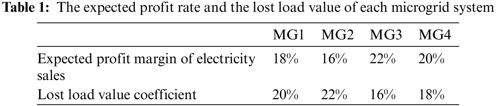
Figure 5: Wind power and photovoltaic power forecast

Figure 6: Renewable energy output and cold, heat and power load data of four microgrid systems

Figure 7: The electricity price curve between the upper microgrid system and the main grid transaction

5.2 Analysis of Results

The effectiveness and practicability of the proposed model are verified by constructing comparative scenarios. Scenario 1: Each microgrid system directly purchases and sells electricity with the main network on the basis of the optimization of the lower level, without considering the interaction between each microgrid system. Scenario 2: The model proposed in this paper.

Through the lower-level optimization, the optimal output combination of the four microgrid systems at each time and the system power surplus or gap amount are obtained. In Figs. 8a–8d, there are four microgrid systems. The gray shaded area represents the overall electrical load of the system during the day (The power load to be calculated in the microgrid system includes not only the power load in the load curve but also the partial energy demand derived from the power supply and the battery charging energy demand in the cold load). Red and green respectively indicate wind power and photovoltaic output. Cyan and blue indicate the amount of battery output and the load reduction of demand response. Yellow is the output of the gas turbine under the minimum constraint of total system cost (Gas turbine plays the role of peak shaving). It can be seen from the figure that the output of the microgrid system at all times does not exceed the comprehensive electrical load curve. It means that the constraint conditions that the gas turbine will no longer output when the system output and the comprehensive electrical load are equal are satisfied. At this time, the remaining output of the gas turbine is the electricity that the system can sell at this time. This part can be calculated according to the gas turbine climbing power constraints and maximum output constraints. When the output of the microgrid system is less than the integrated electrical load phase, it indicates that the gas turbine of the system has reached the maximum output and still cannot meet the power demand. The unsatisfied demand at this time is that the system needs to purchase electricity at that moment. The electric energy that each microgrid system needs to trade with external devices is shown in Fig. 9.

Figure 8: The output of each part of the four microgrid systems and comprehensive electrical load data

Figure 9: Electric energy data of four microgrid systems that need to interact with the outside world

As shown in Fig. 9, the four curves are the electrical energy that the four microgrid systems need to trade with the outside world at each moment. The positive semi-axis of the y-axis represents the surplus part of the microgrid system power. The negative semi-axis of the y-axis represents the power gap of the microgrid system. The curves of MG-1 and MG-3 fluctuate greatly. There are more moments when you need to purchase electricity from the outside world. There are also more moments to sell electricity to the outside world. The overall power supply capacity of MG-2 is greater than its own load level. MG-2 can sell electricity to the outside most of the time. MG-4 needs to purchase electricity from outside most of the time. The above electricity transaction needs to be completed through the upper transaction.

Fig. 10 shows the electric energy trading diagram of four micro grid systems that do not participate in micro grid community transactions and directly conduct electricity purchase and sale transactions with the main grid. The green bar graph is the electricity that the microgrid system sells to the main grid at all times. The orange bar graph is the electricity purchased from the main grid at each moment in the microgrid system.

Figure 10: Electric energy transaction data of 4 MG directly trading with the main grid (Scenario 1)

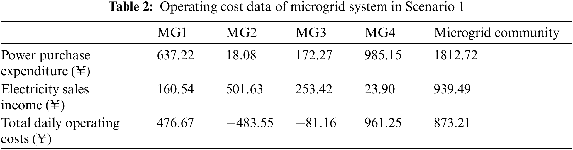
According to the purchase and sale electric energy of the main grid, the income and cost of each microgrid system when directly trading with the main grid are calculated as follows.

In terms of the stable operation of the main grid, it can be seen from the comparison between Figs. 10 and 11 that the development of electric energy transactions in micro-grid communities can form the space-time complementarity between micro-grids, effectively reduce the number of electric energy transactions and trading volume between the micro-grid system and the main grid, which is conducive to the safe and stable operation of the large grid.

Figure 11: Electric energy transaction of 4 MG directly trading with the main grid and other MGs (Scenario 2)

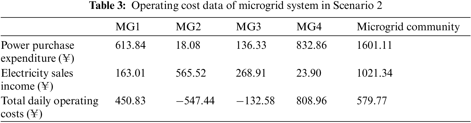
In terms of economic index analysis, the income of microgrid system in Scenario 2 is shown in Table 3.

According to the comparison between Tables 2 and 3, through the model constructed in this paper, intra-community transactions can effectively improve the overall economic benefits of all micro-grid systems in micro-grid communities.

6  Conclusion

This paper proposes a bi-level energy management model, which is suitable for grid-connected MGC with a high proportion of renewable energy. In the optimization of a single microgrid at the lower-level, with the goal of minimizing the total system cost, the start-stop and output of each energy facility are optimized to obtain the optimal output status of each energy facility and the power shortage/surplus of the microgrid. On the upper level, the transaction optimization within the MGC aims to maximize the overall social welfare of the community. By guiding the microgrid to conduct the electricity transaction within the community by means of matching average distribution, and then conduct energy interaction with the main grid, the optimal electricity purchase and sale direction and corresponding electricity quantity of each microgrid are obtained. Then, two typical scenarios are designed to verify the validity of the proposed model. The simulation results show that the bi-level energy management model of MGC-main grid can improve the utilization rate of internal energy facilities of microgrid and significantly reduce the total electricity cost of MGC by first matching the internal electricity transaction of MGC and then trading with the main grid. In addition, transactions at the MGC level can reduce the amount of electricity transactions and the number of transactions between the microgrid and the main grid, promote the stable operation of the main grid to a certain extent, and realize friendly interaction between the MGC and the main grid.

Funding Statement: This paper is supported by Science and Technology Project of State Grid (The construction of provincial energy big data ecosystem and the application practice research of data value-added service for the park, 5400-202012224A-0-0-00).

Conflicts of Interest: The authors declare that they have no conflicts of interest to report regarding the present study.

This work is licensed under a Creative Commons Attribution 4.0 International License, which permits unrestricted use, distribution, and reproduction in any medium, provided the original work is properly cited.