| Energy Engineering |
DOI: 10.32604/ee.2022.017618
ARTICLE
Experimental Performance Analysis of a Corrugation Type Solar Air Heater (CTSAH)
1Ministry of New and Renewable Energy, Government of India, New Delhi, 110003, India
2Department of Green Energy Technology, Madanjeet School of Green Energy Technologies, Pondicherry University, Puducherry, 605014, India
*Corresponding Author: Aravindh Madhavankutty Ambika. Email: aravindh.mnre@gov.in
Received: 25 May 2021; Accepted: 26 August 2021
Abstract: This paper explains the experimental performance evaluation of a Corrugated Type Solar Air Heater (CTSAH) for understanding its performance in a humid tropical climatic condition in Puducherry, India. This helps in understanding its effectiveness in using it for drying application of products like seafood, etc. Experiments were conducted at different mass flow rates and their effect on the heat gain, efficiency, friction factor heat transfer, etc., was analyzed. Experiments were carried out at different mass flow rates, i.e., M1 = 0.06 kg/s, M2 = 0.14 kg/s, M3 = 0.17 kg/s, M4 = 0.25 kg/s, M5 = 0.3 kg/s, and were conducted from 11:00 h to 14:00 h. The air inlet & air temperature is found to be at an average of 40°C whereas the incident solar radiation is at an average of 795 W/m2. Experimental results show that the optimum performance of the CTSAH is in the mass flow rate range of 0.14–0.25 (kg/s). Also, the calculated useful heat produced, convective heat transfer coefficients, effective efficiency, optical efficiency provides knowledge on the potential use of the air heater.
Keywords: Solar air heater; performance analysis; efficiency; solar thermal
The fast-growing population and increasing industrialization have led to the overutilization of fossil fuels for meeting our energy demand and thereby leading to environmental degradation. Therefore, there is a great need to explore and develop renewable energy sources such as solar technology to cope up with the energy demand in the present context [1].
Solar energy is the world’s most incessant source of energy [2] and also the most abundant renewable energy source emitting energy at a rate of 3.8 × 10²³ kW/s of which, approximately 1.8 × 10¹⁴ kW/s is intercepted by the Earth [3]. This amount (60%) of solar energy that reaches the Earth’s surface is very extensive that in one year time it is about twice as much as that will ever be obtained from all other combined Earth's non-renewable resources such as coal, oil, natural gas, and mined uranium. India, a country that has on an average three hundred sunny days per year and receives average hourly radiation of 200 MW/km, has enormous potential for Solar Energy utilization.
A solar air heater is a simple device, which converts solar energy into heat energy. They are being designed and used since the late 19th century when the first accredited solar air heater was designed by Morse [4]. Several models and types of solar air heaters are developed and patented by many researchers for different applications.
The advantages of using SAHs are they are simple in design, have less maintenance, lower corrosion compared to water heaters, and are cost-effective. However, lower thermal properties of air are the important limitation of SAHs. This will increase the amount of air to be handled, increasing the pumping power which in turn reduces the performance of the SAHs. Therefore, proper designing is required for better heat transfer, thereby leading to good efficient performance [5].
Performance improvement can be achieved by using diverse materials, various shapes, and different dimensions and layouts of the components of a solar air heater. Factors such as the type of absorber plate, glass cover plate, and wind speed, affecting the solar air heater efficiency can be varied and modified accordingly [6–10]. However, the scope of the literature review in this may be limited to solar air heaters with corrugated absorber plates. Available relevant literature is reviewed for understanding the aspects of this type of solar air heaters.
Kabeel et al. [11] designed v-Corrugated Plates solar air heater which was experimentally investigated under a wide range of air mass flow rates and operating conditions. The results indicated that the thermal efficiency of the v-corrugated solar air heater was 8%–14.5% more than flat plate solar air heaters and the convective heat transfer coefficient reached up to 1.64 times more than flat plate solar air heaters when the mass flow rate was 0.062 kg/s under the considered configurations and operating conditions. El-Sebaii et al. [12] investigated the double pass flat and v-corrugated plate solar air heaters theoretically and experimentally. The results showed that the double pass v-corrugated plate solar heater was 11%–14% more productive compared to the double pass flat plate solar air heater. This study is to understand the thermal performances of a Corrugation Type Solar Air Heater (CTSAH) through experimental analysis in the tropical weather conditions of Puducherry, India. This study is to understand the usability of solar air heaters for developing indirect type dryers for drying of local products like food items especially seafood, Puducherry, being a coastal area. Such a study will help in developing indigenous models of solar-based dryers with readily available materials which in turn helps to reduce the cost of manufacturing.
2 Design and Development of SAHs
Corrugation Type Solar Air Heater (CTSAH) was designed and installed in the premises of Pondicherry University (12.01° N, 79.85° E). Pondicherry has a great solar energy potential due to its relatively high solar irradiance average measuring about 5.36 kWh/m2/day, which serves as an enormous capacity for solar energy extraction [13]. The SAH is installed in the shadow-free area at an inclination of 12°C. The dimensions and features of the SAH are given in Table 1.
Fig. 1 shows the schematic of the experimental setup with all measuring devices [14]. The corrugated stainless steel is used as the absorber plate. A corrugated sheet made of Aluminium (Al) having 20 SWG thickness is used as the absorption plate with a selective coating to improve the absorptivity of the plate. This absorber plate is packed inside the collector with insulations at the back and sides to reduce heat loss. The absorber plate is positioned such that the air flows above and below the absorber plate. A solar-grade glass of high transmissivity is used as glazing, which helps in increasing the transmittance of incoming solar radiance into the absorber plate and also in blocking the reflected radiation from the absorber plate. A trapezoidal-shaped mixing chamber is connected at the exit of the collector which acts as a convergence point for the proper mixing of outlet air. The outlet of this trapezoidal section is then connected to a multispeed exhaust blower. The blower provides the negative pressure inside the SAH which helps in sucking the air into it through the inlet. An anemometer is used to measure the velocity of the air inside the collector and is measured near the trapezoidal area. A pyranometer is also placed along the trapezoidal area for the measurement of solar radiation available near the surface of the collector. A data logger is connected for continuous measurement of the temperatures and the PT-100 sensors are assigned to measure the inlet air temperature, outlet air temperature, absorber plate temperature, back plate temperature, glazing temperature, and ambient temperature. A pressure measuring instrument is connected to monitor the pressure difference at different sectors within the air heater.


Figure 1: Schematic of the test setup [14]
Fig. 2 shows the experimental setup of the solar air heater.

Figure 2: Experimental setup (a) Cross-section of CTSAH (b) Original experimental setup (inside: photo of cross-section)
3 Performance Evaluation of Solar Air Heaters
Consider a solar air collector with collector area
where the useful heat gain,
To understand the economic performance of the solar air heater, the pumping power used for the active circulation should also be considered, thereby the thermal efficiency becomes effective efficiency and is given by [16]
where
Pumping power is the amount of energy required for running the electric fan/blower for operating the solar air heaters in turbulence mode and can be found using the formula [17]
where Q is the volume flow rate and
The pressure drop
For corrugated type SAH, the friction factor is [18]
The thermal performance can be well understood by deriving the heat transfer equation for different components of the SAHs. At the glazing, the overall heat transfers can be expressed as
The radiative heat coefficient
And the radiative heat transfer coefficient
where
The convective heat transfer coefficient
where
The convective heat transfer coefficient
where the hydraulic diameter
At the absorber plate, the heat balance equation can be expressed as
The convective heat transfer coefficient
where
At the back plate, the expression is
The conductive heat transfer
The heat gained by the fluid is the sum of the convective heat transfer from the glazing, absorber plate, and back plate to the air and is given by the formula
Reynolds number for the air passage in corrugated solar air heater is [23]
For the upper air passage, the hydraulic diameter,
The density
Experiments are conducted in an open-loop as per the ASHRAE 93-1986 (RA 91) standards [26]. Solar irradiance is measured using a pyranometer with a measuring range of 0–2000 W/m2 and sensitivity of 10 μV/(W/m2) positioned in the same slope as that of the test setup. Provision for measurement of the temperature of inlet and outlet air, glazing, absorber plate, the back plate is also made. The ambient temperature is also measured as per the standards. RTD type temperature sensors having a measuring accuracy of 0.1°C are used along with a data logger is used for measuring the temperature. The data logger is provided with 16 input channels thereby multiple sensors can be connected to it. A digital anemometer with a measuring range of 0 to +20 m/s and resolution of 0.01 m/s is used for measuring the air velocity and the pressure drop is measured using a digital differential pressure gauge with a range of 0 to 100 hPa and resolution of 0.01 hPa.
Experiments are conducted simultaneously to understand the performance of the CTSAH at five different mass flow rates (M1 = 0.06 kg/s, M2 = 0.14 kg/s, M3 = 0.17 kg/s, M4 = 0.25 kg/s, M5 = 0.3 kg/s). The entire test setup is made to operate for at least 30 min before the start of the experiments for reaching steady-state conditions. The measurements are made from 11:00 to 14:00 h for the analysis. The measured solar radiation (I) for all the experiment dates is plotted against the time shown in Fig. 3.

Figure 3: Time vs. solar radiation (all speeds)
The above graph indicates a pictorial representation of the solar intensity at different speeds of the blower operated. The graphs show different peaks due to the difference in solar radiation of that particular day. Apart from that, the graphs show similar nature of the curve, that is, they gradually increase till noon and then show a consistent manner of decline post noon, The solar radiation measured during the experiment was in the range 664–904 W/m2 with average solar radiation of 795 W/m2.
Fig. 4 shows the time vs ambient temperature (Ta) during the experiment dates. The ambient temperature (Ta) was always found to be between 30.5°C–36.1°C during the measuring period with an average of 32.9°C. It was observed that the peak ambient temperature is also occurring between 12:00 h and 13:00 h. Temperature and solar radiations are measured at different blower velocities and are plotted against time. Fig. 5 shows a time vs. temperature & solar radiation plot for the CTSAH for different speeds.

Figure 4: Ambient temperature (Ta) vs. time

Figure 5: Temperature & solar radiation vs. time plot for the CTSAH
The above graphs are shown for different mass flow rates with M1 being the lowest and M5 being the highest of the mass flow rates. Black represents ambient temperature, red is for plate temperature, blue for inlet temperature, pink for outlet temperature, and green for irradiance. For M1, the ambient temperature is always above 30°C and is in the range of 32°C–35°C. The inlet temperature is found in the range of 38°C–41°C with an average of 40°C. The plate temperature is always above 80°C and reaches the maximum of 83.3°C at 12:30 h. The outlet temperature is in the range of 65°C–70°C. Solar radiation is at its peak at noon of 825 Wm−2.
For speed M2, the ambient temperature is again at the average of 32°C and is always above 30°C. Inlet air slightly increases as the day progresses. The peak is seen around 13:00 h. it starts from just below 40°C and reaches up to 42°C, the plate temperature on the other hand starts from just below 80°C and the peak is seen around 12:25 h of 84°C. Outlet temperature goes up to 77°C and decreases after 13:15 h. Solar irradiance is a plateau in nature rather than a peak of maximum irradiance of 815 Wm−2 is seen at 12:30 h.
Here is speed M3, the solar radiation is at around 778 Wm−2 in turn reducing the temperatures. However, the ambient temperature is still found to be at an average of 32°C. The inlet temperature starts from just under 40°C and goes up to 41°C at maximum. The plate temperature reading gradually rises to 80°C and decreases as the day passes by giving the average output temperature of 72°C. No significant peaks are seen.
With the peak of solar radiation hitting a peak mark of 828 Wm−2, the plate and outlet temperatures are to rise. The ambient temperature stayed above 30°C on an average of 32°C. The inlet temperature is at an average of 40°C. The plate temperature starts rising from just above 80°C and always stays there with the temperature reaching 82°C between 12:00–13:00 h. The outlet temperature is averaged to be around 72°C and is always above 70°C with a maximum being 75°C.
There is not much difference in the ambient and the inlet temperature when it comes to speed M5. However, the inlet temperature averages just below 40°C at around 38°C. The solar radiation has hit a peak of 900 Wm−2 with the radiation being more than 875 Wm−2 from 11:45–13:05 h. However, the plate temperature is almost linear with an average temperature of around 81°C. The outlet temperature reaches 70°C during the peak radiation with the average being around 69°C throughout the graph.
Generally, as the air velocity increases, the air output temperature decreases due to lesser time interaction within the system.
The average ambient temperatures and the solar radiation during the experiments with different mass flow rates are shown in Fig. 6. It may be observed that the average absorber plate temperature and the air outlet temperature seem to follow the pattern that of solar radiation. The ambient temperature is a flat line throughout the entire mass flow rate despite hitting the maximum of 35°C at M3. Similarly, the inlet temperature is in the range of 41°C for all mass flow rates. A steep decline in the solar irradiance can be seen for M3 which in turn has reduced both the absorber plate and air outlet temperatures as shown in the graph. However, despite the solar irradiance showing higher values for M5, both the absorber plate and air outlet temperatures have shown a decline.
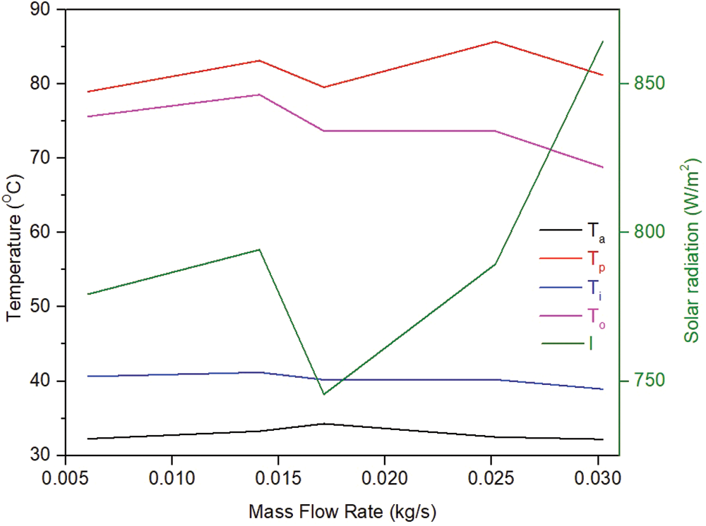
Figure 6: Average temperatures and solar radiations vs. mass flow rate
Fig. 7 shows the time vs. temperature gain (

Figure 7: Temperature gain (
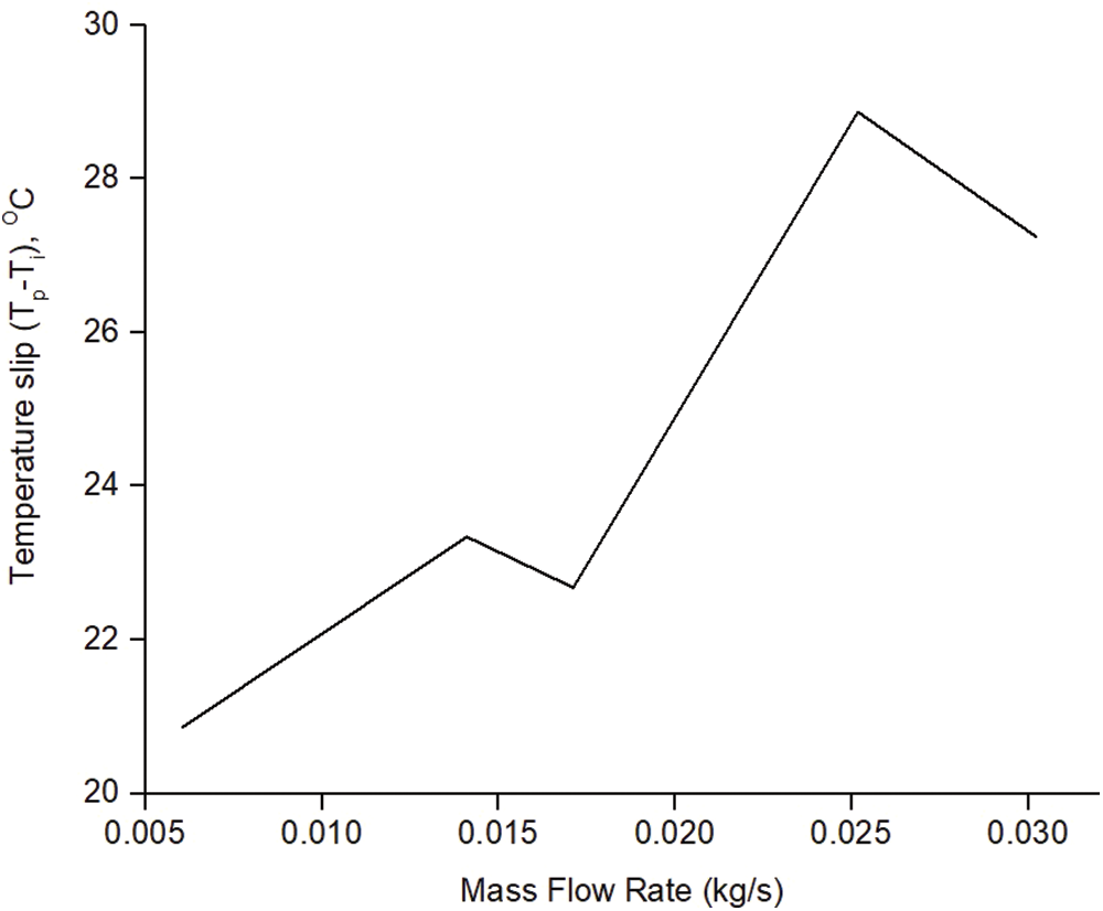
Figure 8: Temperature gain (
The above graph shows a similar behavioural pattern of temperature gain throughout the experimental time duration for different mass flow rates. This shows that the temperature readings are directly proportional to the solar irradiance readings of that particular day. The graphs of temperature gain are also justified by Fig. 8 where average temperature slip has been calculated and plotted against different mass flow rates. The relation between temperature gain and temperature slip is that they are directly proportional to each other.
The above graph is drawn by computing the average temperature slip and is plotted against the mass flow rates. It also follows the solar irradiance readings of that particular day which shows the nature of the decline in the temperature slips for M3. As the absorber plate temperature for M5 was found to be comparatively lesser despite the solar irradiance being higher, the consequence is seen on the graph as a decline at M5. However, the nature of the graph clearly shows that the average temperature slip has increased as the mass flow rates have escalated with the slip temperature reaching 29°C for speed M5. This also means that the temperature gain has increased as the mass flow rates escalated.
Fig. 9 shows the convective heat transfer coefficient and average heat gain for different mass flow rates. From the graph, it is well understood that they are directly proportional. The increment in the convective heat transfer coefficient is due to the higher heat transfer, promoted turbulence, and higher efficiency. This leads to an increment in useful heat collected by the absorber plate. Additionally, heat loss from the collector also decreases.
The pumping power and the friction factor are calculated from the measured pressure drop using formulas (4) and (5) and plotted as the graph shown above. Fig. 10 shows the friction factor vs. Reynolds number. As per the plot, the friction factor seems to be reduced for higher mass flow rates. This shows that as the heat transfer coefficient and the useful heat gain increase, the heat loss and frictional loss significantly decrease.

Figure 9: Convective heat transfer coefficient and average heat gain vs. mass flow rate

Figure 10: Friction factor vs. Reynolds number
The efficiency of the solar air heater is calculated using the heat gained, pumping, and the incident solar radiation and is plotted against different mass flow rates and is shown in Fig. 11. The linear graph has a positive inclination throughout the different mass flow rates, which means the gain in useful heat trapped inside the absorber plate and the increment in convective heat transfer, in turn, increases the effective efficiency of the solar air heater. The effective efficiencies for M1, M2, M3, M4, and M5 are 16%, 39%, 46%, 64%, and 61%, respectively. The efficiency for M5 has shown a decline due to the decrement in the absorber plate and the air outlet temperatures.

Figure 11: Efficiency vs. mass flow rate
The outlet fluid temperature of the v-corrugated solar heater developed by Kabeel et al. is in the range of 20%–50% [11] and by El-Sebaii et al. is in the range of 52%–65% [12], which is comparatively similar in the range of this paper.
5 Efficiency Curves
The effective efficiencies are calculated and,

Figure 12:
Regression lines are shaped by using the line of best fit of least squares. The generated lines have negative slopes for the absorber plates as shown in Table 2 below. Optical efficiency

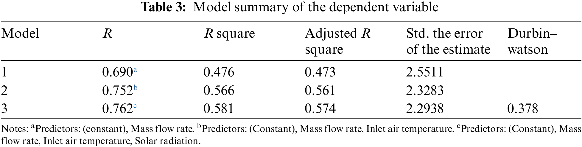
In this study, the outlet air temperature is the dependent variable, and mass flow rate, inlet air temperature & solar radiation are independent variables. Analysis of Variance (ANOVA) is done to understand the quality of prediction of the dependent variable, which can be determined from the R-value from multiple regression analysis.
From Table 3 above, it can be seen that the 0.690, 0.752, and 0.762 give a good level of prediction of mass flow rate, mass flow rate–inlet air temperature, and mass flow rate–inlet air temperature–solar radiation, respectively.
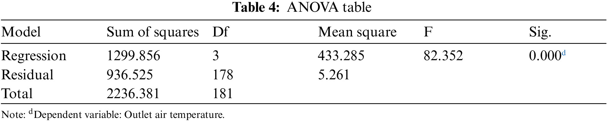
The F ratio in Table 4 shows that the overall regression model is good for the data. The significant value of the dependent variable shows that it can be predicted statistically using the independent variables.
The performance of a simple CTSAH is evaluated using the experimental method for different mass flow rates, which shows the following results for the SAH:
• The graphs show that the temperature readings are directly proportional to the solar irradiance for that particular day. Also, the absorber plate and outlet temperatures show an average of 80°C and 75°C respectively and tend to decline for higher mass flow rates. This is because, as the air velocity increases, the air output temperature decreases due to lesser time interaction within the system.
• It is also observed that the temperature readings directly rely on the solar irradiance of that day. The decline in solar irradiance has shown decrement in the absorber plate and the air output temperatures. Apart from speed M5 showing a decrement in both the absorber plate and air outlet temperature despite solar irradiance hitting the peak mark of 900 Wm−2, the rest of the temperature graph is directly proportional to that of the solar irradiance with the temperature gain (
• Another observation is that temperature gain is directly proportional to the average temperature slip which is the arithmetic difference between the absorber plate temperature and the air inlet temperature. Fig. 8 shows the graph plotted between the temperature slip and the mass flow rates. The inclined linear graph of temperature slip against the increasing mass flow rate shows that there is a gain in temperature as the mass flow rate increases. The decline in the graph at M3 is due to the decrement of solar irradiance.
• The experiment also shows that an increment in convective heat transfer coefficient and the useful heat gain in the SAHs are directly proportional to the increment in mass flow rates. The increment in the convective heat transfer coefficient is due to the higher heat transfer, promoted turbulence, and higher efficiency and reaches a maximum value of 19.5 Wm−2 °C−1. This leads to an increment in useful heat collected by the absorber plate which has a maximum value of 925 W. In addition to this, there is a decrement in heat loss as the convective heat transfer coefficient increases.
• The experiment is proof of decrement in the heat losses and the frictional losses as well. As per the plot, the friction factor seems to be inversely proportional to Reynolds number associated. The values of friction factor for 375 and 1700 Reynolds numbers are 0.0185 and 0.0135, respectively.
• It was found that effective efficiency increases as the mass flow rate increases which mean the gain in useful heat trapped inside the absorber plate and the increment in convective heat transfer, in turn, increases the effective efficiency of the solar air heater with the values being 16%, 39%, 46%, 64% and 61% for M1, M2, M3, M4, and M5, respectively.
• It was seen that optical efficiency is obtained at the intersection of the lines of best fit with the vertical axis. The negative slopes shown in Table 2 corresponds to the absorber plate’s overall heat transfer coefficient.
Considering the experiment, it is understood that higher turbulence, higher heat transfer, and higher efficiencies are received as the mass flow rate is increased. The design and construction of these types of solar air heater are simple and has very less maintenance. It can be easily constructed with easily available manufacturing materials and therefore can be utilized for drying applications. However, the operational conditions may be optimized as required for the drying product.
Funding Statement:Authors thank the Department of Science and Technology, Government of India (https://www.dst.gov.in) for the Grant No. SR/FTP/ETA-0064/2014 granted to Sreekumar, A.
Conflicts of Interest: The authors declare that they have no conflicts of interest to report regarding the present study.
1. Khalil, A. (2016). Investigation of the thermal performances of flat, finned, and v-corrugated plate solar air heaters. Journal of Solar Energy Engineering, 138(5), 1–7. DOI 10.1115/1.4034027. [Google Scholar] [CrossRef]
2. Kabeel A. E., Arunkumar T., Denkenberger D. C., Sathyamurthy R. (2017). Performance enhancement of solar still through efficient heat exchange mechanism—A review. Application Thermal Engineering, 114, 815–836. DOI 10.1016/j.applthermaleng.2016.12.044. [Google Scholar] [CrossRef]
3. Singh, N. K., Kumar, J. (2019). Solar air heater duct with wavy delta winglets: Correlation development and parametric optimization: A review. International Journal of Advanced Computer Technology, VIII(12), 9–12. DOI 10.1007/s00231-019-02651-9. [Google Scholar] [CrossRef]
4. Saxena, A., El-Sebaii, A. A. (2015). A thermodynamic review of solar air heaters. Renewable and Sustainable Energy Reviews, 43(1), 863–890. DOI 10.1016/j.rser.2014.11.059. [Google Scholar] [CrossRef]
5. Garg, H. P., Prakash, J. (2000). Solar energy: Fundamentals and applications. New Delhi: Tata McGraw-Hill. [Google Scholar]
6. Wilhelm, L. R., Suter, D. A., Brusewitz, G. H. (2004). Food & process engineering technology, St. Joseph, MI: American Society of Agricultural Engineers. https://www.asabe.org/media/184966/chapter_10_in_wilhelm_food_proc._eng._tech.pdf. [Google Scholar]
7. Saini, R. P., Singal, S. K. (2007). A review on roughness geometry used in solar air heaters. Solar Energy, 81(11), 1340–1350. DOI 10.1016/j.solener.2007.01.017. [Google Scholar] [CrossRef]
8. Aravindh, M. A., Sreekumar, A. (2016). Efficiency enhancement in solar air heaters by modification of absorber plate: A review. International Journal of Green Energy, 13(12), 1209–1223. DOI 10.1080/15435075.2016.1183207. [Google Scholar] [CrossRef]
9. Tyagi, V. V., Panwar, N. L., Rahim, N. A., Kothari, R. (2012). Review on solar air heating system with and without thermal energy storage system. Renewable and Sustainable Energy Reviews, 16(4), 2289–2303. DOI 10.1016/j.rser.2011.12.005. [Google Scholar] [CrossRef]
10. Yadav, A. S., Bhagoria, J. L. (2013). Heat transfer and fluid flow analysis of solar air heater: A review of CFD approach. Renewable and Sustainable Energy Reviews, 23(2), 60–79. DOI 10.1016/j.rser.2013.02.035. [Google Scholar] [CrossRef]
11. Kabeel, A. E., Khalil, A., Shalaby, S. M., Zayed, M. E. (2016). Experimental investigation of thermal performance of flat and v-corrugated plate solar air heaters with and without PCM as thermal energy storage. Energy Conversion and Management, 11(4), 264–272. DOI 10.1016/j.enconman.2016.01.068. [Google Scholar] [CrossRef]
12. El-Sebaii, A. A., Aboul-Enein, S., Ramadan, M. R. I., Shalaby, S. M., Moharram, B. M. (2011). Investigation of thermal performance of double pass-flat and v-corrugated plate solar air heaters. Energy, 36(2), 1076–1086. DOI 10.1016/j.energy.2010.11.042. [Google Scholar] [CrossRef]
13. Acharya, D., Gautam, K., Prasath, A. (2017). Feasibility study of solar power plant for Pondicherry University. International Journal of Science and Research, 6, 406–411. DOI 10.21275/1081702. [Google Scholar] [CrossRef]
14. Rajarajeswari, K., Alok, P., Sreekumar, A. (2018). Simulation and experimental investigation of fluid flow in porous and non-porous solar air heaters. Solar Energy, 171(7), 258–270. DOI 10.1016/j.solener.2018.06.079. [Google Scholar] [CrossRef]
15. Bharadwaj, S. S., Singh, D., Bansal, N. K. (1981). Design and thermal performance of a matrix solar air heater. Energy Conversion Management, 21(4), 253–256. DOI 10.1016/0196-8904(81)90021-2. [Google Scholar] [CrossRef]
16. Cortés, A., Piacentini, R. (1990). Improvement of the efficiency of a bare solar collector using turbulence promoters. Applied Energy, 36(4), 253–261. DOI 10.1016/0306-2619(90)90001-T. [Google Scholar] [CrossRef]
17. Mittal, M. K. K., Varshney, L. (2006). Optimal thermohydraulic performance of a wire mesh packed solar air heater. Solar Energy, 80(9), 1112–1120. DOI 10.1016/j.solener.2005.10.004. [Google Scholar] [CrossRef]
18. Darici, S., Kilic, A. (2020). Comparative study on the performances of solar air collectors with trapezoidal corrugated and flat absorber plates. Heat and Mass Transfer, 56(6), 1833–1843. DOI 10.1007/s00231-020-02815-y. [Google Scholar] [CrossRef]
19. Zhai, X. Q., Dai, Y. J., Wang, R. Z. (2005). Comparison of heating and natural ventilation in a solar house induced by two roof solar collectors. Applied Thermal Engineering, 25(5–6), 741–757. DOI 10.1016/j.applthermaleng.2004.08.001. [Google Scholar] [CrossRef]
20. Swinbank, W. C. (1963). Long-wave radiation from clear skies. Quarterly Journal of the Royal Meteorological Society, 89, 339–348. DOI 10.1002/(ISSN)1477-870X. [Google Scholar] [CrossRef]
21. Kays, W. M., Crawford, M. E. (1980). Convective heat and mass transfer. New York: McGraw-Hill. [Google Scholar]
22. Hollands, K. G. T., Shewen, E. C. (1981). Optimization of flow passage geometry for air-heating, plate-type solar collectors. Journal of Solar Energy Engineering, 103(4), 323–330. DOI 10.1115/1.3266260. [Google Scholar] [CrossRef]
23. Liu, T., Lin, W., Gao, W., Luo, C., Zheng, M. Li et al. (2007). A parametric study on the thermal performance of a solar air collector with a v-groove absorber. International Journal of Green Energy, 4(6), 601–622. DOI 10.1080/15435070701665370. [Google Scholar] [CrossRef]
24. Ong, K. S. (1995). Thermal performance of solar air heaters: Mathematical model and solution procedure. Solar Energy, 55(2), 93–109. DOI 10.1016/0038-092X(95)00021-I. [Google Scholar] [CrossRef]
25. Bolz, R. E. (2019). CRC handbook of tables for applied engineering science. CRC Press. DOI 10.1201/9781315214092. [Google Scholar] [CrossRef]
26. ANSI/ASHRAE 93-1986 (R1991)-Standard 93-1986 (R1991). Methods of testing to determine the thermal performance of solar collectors. American Society of Heating, Refrigerating, and Air-Conditioning Engineers. [Google Scholar]
 | This work is licensed under a Creative Commons Attribution 4.0 International License, which permits unrestricted use, distribution, and reproduction in any medium, provided the original work is properly cited. |