| Energy Engineering |
DOI: 10.32604/ee.2022.018913
ARTICLE
Development of Vehicle-to-Grid System to Regulate the System Parameters of Microgrid
1Power System Planning Division, Rajasthan Rajya Vidyut Prasaran Nigam, Ltd., Vidyut Bhawan, Japur, India
2Department of Electrical and Computer Engineering, Hawassa University, Hawassa, Ethiopia
3Electrical Engineering Department, School of Engineering, University of Petroleum and Energy Studies, Dehradun, India
*Corresponding Author: Baseem Khan. Email: baseem.khan04@ieee.org
Received: 24 August 2021; Accepted: 11 November 2021
Abstract: This paper proposes a vehicle-to-grid (V2G) system interfaced with a microgrid that is effective at regulating frequency on a microgrid over a 24-h cycle. A microgrid is designed and divided into four components. The first component is a diesel generator, which is used to act as the base power generator. The second component consists of renewable energy (RE) power plants, which include solar photovoltaic (PV) and wind plants. The third component is a V2G system. The last component is the load connected to the microgrid. A microgrid is designed to be of sufficient size to represent a community of one thousand households during the day period of low consumption in the spring or fall seasons. A hundred electric vehicles (EVs) are modeled as base models to realize a 1:10 ratio for cars to households, which indicates a possible scenario in the near future. Detailed analysis of the active power, reactive power, voltage, frequency, and current is carried out. It is established that the proposed design of the V2G and microgrid effectively maintains system parameters such as frequency and voltage within permissible limits with an error of less than 1%. Further, transient deviations in these parameters are limited to within 5%. A microgrid with V2G devices regulates the system frequency by mitigating load demand through coordinated control of conventional generation, solar PV plant generation, wind plant generation, power exchange with the microgrid network, and electric vehicles. The proposed microgrid and V2G are efficient for energy management and mitigation of intermittency and variability of RE power with improved performance. Variations in system parameters have been investigated by changing the operating scenario, and it has been determined that the error is limited to less than 5%. The study is effectively realized in the MATLAB/Simulink environment.
Keywords: Microgrid; electric vehicles; vehicle-to-grid; renewable energy; PV; wind
Nomenclature
| AP | Access point |
| AS | Ancillary service |
| ASM | Asynchronous machine |
| BESS | Battery energy storage systems |
| BEV | Battery electric vehicle |
| BMS | Battery management system |
| CAC | Channel access control |
| CAN | Controller area network |
| DER | Distributed RE resources |
| DG | Distributed generators |
| DGR | Diesel generator |
| DLC | Direct load control |
| DMPC | Distributed model predictive control |
| DR | Demand response |
| DRX | Delay response cross layer |
| EDRX | Equal and delay response cross layer |
| EV | Electric vehicle |
| FCR | Frequency containment reserve |
| G2V | Grid to vehicle |
| HAN | Home area network |
| HEV | Hybrid electric vehicle |
| ICV | Internal combustion vehicle |
| IEEE | Institute of Electrical and Electronics Engineers |
| PEM | Proton exchange membrane |
| PEV | Plug-in electric vehicle |
| PHEV | Plug-in hybrid electric vehicle |
| PHS | Pumped hydro storage |
| PV | Photovoltaic |
| QCEV | Quality of service scheme to charge EVs |
| QoS | Quality of service |
| RE | Renewable energy |
| SOC | State of charge |
| V2B | Vehicle-to-building |
| V2G | Vehicle-to-grid |
| VPP | Virtual power plant |
| WAVE | Wireless access in vehicular environment |
| WECS | Wind energy conversion system |
| WSANs | Wireless sensor and actor networks |
A microgrid is an electricity network that intelligently combines the activities of all linked generators, including conventional and distributed generators (DG), users, and consumers, to efficiently deliver a reliable, cost-effective, and stable electricity supply to consumers. This smart micro-grid combines innovative devices and services with intelligent monitoring, control, communication, and self-healing technologies to (i) enable integration and operation of the generators of all sizes and technologies; (ii) enable consumers to actively participate in the system operation; and (iii) significantly reduce the system's environmental impact [1]. Hybrid energy systems have recently been described as an effective solution for mitigating the power supply issues and challenges due to the intermittency and unpredictability of solar and wind energy. This results in the requirement for backup energy resources. Hence, energy storage systems are often needed when utilizing RE resources. During the period of non-availability of RE, the backup energy resource is used to provide energy. This also helps to solve the problems of activities related to demand-side management of the power system. Electric vehicle to grid (V2G) is a term related to an energy storage technology that allows bidirectional power transfer between a V2G battery and the power grid. With V2G capability, the state of charge of a V2G battery will go up or down depending on revenues and grid demands. As a result, charging and discharging of V2Gs has the power to make a V2G parking lot a controllable load [2]. Various aspects of electric vehicles are the subject of investigations. In [3], Noel et al. presented 227 reviews of transportation and electricity from 200 institutions across the Nordic region and summarized the extensive range of benefits for both EVs and V2G. This study also presents 29 and 25 types of benefits for EVs and V2G, respectively, which have various benefits, including cost savings, reduced emissions, and the introduction of renewable energy. The most common EV gain is noise reduction, which has been proven. A comparative and mixed evaluation framework for various dimensions of electric mobility and specified preferences for electric vehicles in the Nordic zone are detailed in [4]. This involves the possibility of configuring the existing vehicles into V2G vehicles, which can store energy and provide grid services, generating revenue and hastening decarbonization. Sovacool et al. [5] presented a study to explore the possibility of mobilizing large flows of investment and finance, as well as private sector commitment, to decarbonize passenger transportation in Europe. The types of actors and stakeholder groups, business models, and resulting innovation activity structures that help to build or accelerate V2G technology are discussed. This study assesses stakeholder perceptions of primary and secondary business models for V2G. This was achieved using qualitative research interviews and focus groups in five countries—Denmark, Finland, Iceland, Norway, and Sweden—as well as a systematic literature review.
Research activities reported in the fields of microgrid and vehicular technologies are discussed in this section. A detailed review of literature related to the V2G technology is included in this section.
1.1.1 Review of Literature Related to Microgrids
Grid-connected RE sources such as wind and solar power, as well as new loads (electric vehicles and heat pumps), are expected to pose significant challenges to electric power networks around the world [6]. The most effective approach is to convert the current power system infrastructure into a microgrid, which is an intelligent energy grid. It has been described as a novel power grid that includes smart metering infrastructure capable of sensing and measuring power consumption by users using advanced information and communication technologies, with the goal of completely upgrading energy generation, transmission, and distribution [7,8]. Demand response (DR), RE sources, V2G capacity, microgrid, advanced metering, two-way communications, and other smart grid features are important features of the micro-grid [9]. The smart grid has also been recognized as a new field and incorporates new analysis, control, instrumentation, and security functions. Its key goals are to improve the efficiency of the power grid to reduce carbon emissions, as well as restrict the expansion of the power network to achieve improved stability, reliability, and market exploration [10,11]. Real et al. [12] introduced an expanded distributed model predictive control (DMPC) paradigm and its applications to the smart grid. A case study is presented which focuses on solving a combination of environmental and economic dispatch dilemmas. Hu et al. [13] describe a smart home test bed for bridging the gap between conventional power systems and modernized smart grids. Chanda et al. [14] suggested an optimization model to optimize social welfare by standardizing operating conditions with an overall improvement in the dynamic stability of power markets using smart grid connectivity technologies. Goulden et al. [15] discussed the role of users in demand-side management of smart grids with the aid of a smart design. Evora et al. [16] described a direct load control (DLC) approach based on a multi-objective particle swarm optimization algorithm for load control in smart grids. Karimi et al. [17] investigated the issue of efficiently concatenating several small smart metering messages arriving at data concentrator units in order to minimize protocol overhead and increase network efficiency. Liang et al. [18] proposed a large-area measurement-based dynamic stochastic optimal power flow control algorithm based on adaptive critical designs to achieve a high penetration level of intermittent RE into smart grids. Milioudis et al. [19] proposed a method for locating high impedance faults in smart grids with pinpoint accuracy. Claessen et al. [20] presented a comparative study of tertiary control systems for micro grids using the flex-street model.
A large amount of work has been published on the different aspects of the smart grid. In [21], Cecati et al. provided an overview of smart grid principles. Tenti et al. [22] proposed a conservative power theory for microgrid regulation that meets our characterization requirements. This also serves as a testing ground for cooperative control strategies for distributed switching power processors and static reactive power compensators. In [23], Gamage et al. presented protection properties for information flow using a confidentiality model, minimizing the event of confidentiality violations in smart grids. This algorithm has been put through its paces on a variety of physical devices, including the IEEE-118 bus test system. Tuballa et al. [24] provided a systematic analysis of developments in the area of smart grid technologies. Al-Anbagi et al. [25] proposed two protocols for wireless sensor and actor networks (WSANs) used in smart grid communication to solve data prioritization and delay-sensitive data transmission. The delay response cross layer (DRX) and equal and delay response cross layer (EDRX) data transmission schemes are used in these protocols. Huang et al. [26] described a priority-based traffic scheduling method for a cognitive radio communication infrastructure-based smart grid system that takes into account heterogeneous characteristics such as control commands, multimedia sensing data, and meter readings. Li et al. [27] suggested an efficient power allocation scheme for downlink capability in a heterogeneous home area network (HAN) with an application to the smart grid. This is achieved by the application of a beam-forming technique to the smart meters. Ancillotti et al. [28] provided a comprehensive description of routing protocols for smart grid applications, as well as a critical review of their benefits and drawbacks. Pang et al. [29] detailed the advantages of battery electric vehicles (BEVs) and plug-in hybrid electric vehicles (PHEVs) as dynamically configurable distributed energy storage in a vehicle-to-building (V2B) operating mode. Deng et al. [30] suggested an online load scheduling solution to mitigate the effect of price prediction errors and temporally coupled constraints in smart grids. Liu et al. [31] proposed a queuing-based energy consumption control scheme for heterogeneous demands in smart grids.
1.1.2 Review of Literature on Vehicular Technology
A brief review of vehicular technology is discussed in this section. Kumano et al. [32] introduced an online load scheduling solution to mitigate the impact of price prediction errors and temporally coupled constraints in smart grids. Krueger et al. [33] proposed a queuing-based energy consumption control scheme for heterogeneous demands in smart grids. Meesenburg et al. [34] defined a delivery of frequency containment reserve (FCR) that is carried out by a fleet of electric vehicles. Further, a large heat pump to take advantage of synergies between fast-regulating batteries and large-capacity heat storage in a thermal device has also been introduced. The feasibility of this approach is evaluated using an EV state of charge model that provides FCR as well as device frequency measurements over a one-year cycle that accounts for charge conversion losses. A dynamic heat pump system model is also used. Experimental data is used to validate these two models. The EVs’ operations are checked in an experimental environment. Al-Anbagi et al. [35] detailed the state-of-the-art for Wireless Access in Vehicular Environments (WAVE) for V2G applications and elaborated on the key challenges associated with WAVE implementation in V2G applications. The QoS scheme to charge EVs (QCEV) in a smart grid scenario and the channel access control (CAC) system are two IEEE 802.11p-based Quality of Service (QoS) methods for enabling interaction between the smart grid and EVs. The IEEE 802.11p MAC protocol is used in traditional distributed QoS techniques. In situations where fast EV battery charging is needed, the QCEV and CAC approaches implement centralized QoS, which distinguishes them. Does the access point (AP) use a central principle to decide whether an EV should be given top priority for accessing a channel that uses individual levels of EV battery or not? This is also supported by the availability of electricity and its cost in different locations. Bamisile et al. [36] presented a report on the use of solar PV plants and onshore wind turbines to produce electricity in an area of the Republic of China. A complex combination of hydrogen production and electric vehicles for the energy mix is modeled. I investigated three types of energy storage mechanisms, including V2G, V2G + battery, and V2G + pumped hydro storage (PHS). Energy-efficient computer codes are created to perform complex simulations in order to conduct research on carbon emissions reduction. PV and on-shore wind power plants with a capacity of 1 TWh/yr are estimated to meet demand of 0.02 TW/yr and EV charging demand of 750 MW, respectively. V2G has a storage capacity of 30 GWh, V2G + Battery has a capacity of 55 GWh, and V2G + PHS has a capacity of 60 GWh, depending on various charge/discharge profiles based on hours. The solution proposed in this study would help to reduce coal consumption by 495.3 kton per year. In [37], Roman et al. proposed a pairing-based authentication protocol that ensures contact confidentiality, protects EV users’ identities, and prevents attackers from monitoring the car. In contrast to other protocols, the results of computing and communications efficiency analyses were higher, resolving signaling congestion and reducing bandwidth usage. A comprehensive security review showed that the protocol protects electric vehicles (EVs) from a variety of known threats and that it meets the security objectives. A comprehensive review of public perceptions of electric vehicles and V2G, taking into account [38], describes the findings of a Nordic focus group report. The authors of [39] presented a study to model and simulate a V2G system in a microgrid network after taking into account the specifications for various components of the microgrid network, such as distributed RE resources (DERs), plug-in electric vehicles (PEVs), and non-PEV loads. The system model is created using an agent-based approach, in which microgrid components are treated as agents. The use of PEV car batteries has been referred to as a “virtual power plant” (VPP), which allows PEVs to function as loads. Wind and solar power plants have been used as energy sources in conjunction with DERs. For continuous integration of a large number of PEVs into a microgrid network, efficient control and scheduling of PEV charging and discharging via charging station applications is used. This analysis also includes a simulation of a microgrid service to show how agents’ behavior changes as a result of factors such as RE penetration, PEVs, PEV driver travel patterns, and energy generation pricing.
Increased concern for the atmosphere and energy protection is aiding in e-mobility research around the world. The main policies in the areas of health, the environment, energy, transportation, and economics are all geared toward promoting continuous mobility [40,41]. RE power-supported e-mobility can assist in achieving zero-emission standards. PEVs rely on fossil fuel-fueled power plants in their early stages. Separating CO2 from these plants’ emissions would aid in the reduction of dispersed emissions from internal combustion vehicles (ICV). Bilgin et al. [42] described the technologies that allow e-mobility. PEVs are useful in supporting the grid on a temporary distributed storage system, and ancillary service (AS) can help to incorporate RE plants by acting as a “shock absorber” [43,44]. There is a proposal in the Balearic touristic islands of Spain to reduce pollution and to replace a large portion of electricity production with renewable energy plants. The use of solar photovoltaic power plants and battery energy storage systems (BESS) is the main priority [45]. Furthermore, when connected to the power grid, PEVs may play an important role. The best use of PEVs for temporary storage devices will reduce the amount of BESS needed and the overall investment costs [46]. In [47], Mohamed et al. proposed a fuzzy cloud stochastic framework for energy management of microgrids with a high RE share, considering the maximum deployment of electric vehicles. This has devised a policy for control of the charging demand in three different schemes, which include the smart scheme, coordinated scheme, and uncoordinated scheme. This technique is effective to capture the influence of uncertainties due to RE generation and to initiate suitable control actions to mitigate these uncertainties. A stochastic scheduling approach for a hybrid microgrid integrating PHEVs to manage charging demands has been designed in [48]. Three charging patterns are introduced, including coordinated, uncoordinated, and smart charging models, with separate characteristics for type of charger, capacity, and market share. RE generation from wind energy conversion systems (WECS), solar PV system panels and fuel cells is taken into consideration for the scheduling process of energy management in the hybrid microgrid. To mitigate the charging effects of EVs on the operation of hybrid microgrids, remote switches are designed for the system, which changes the topology and power flow. A data-driven framework using the point estimate technique and SVM is used to design a scheme for minimizing the effects of uncertainty. The developed approach is stable; the role of switching reduces the operational cost, and it assesses the role of PHEV in the operation of a microgrid. In [49], Gong et al. designed a holistic model for the proton exchange membrane fuel cell that is effective for retrieving the excess thermal energy generated during operational time. This model uses the unutilized capacity of the fuel cell for generating and storing hydrogen, which can be used at a later stage with increased efficiency. Further, a stochastic framework is formulated utilizing the point estimate method for minimizing the effect of uncertainties in solar PV, WECS, forecast error, prices of power utilities, operating temperature of proton exchange membrane (PEM) fuel cells, price for natural gas, price for selling hydrogen, and pressure of H2 and O2 in stacks of fuel cells. The developed approach has the advantages of high accuracy and minimum running time. In [50], Avatefipour et al. suggested an effective method for the detection of anomalies in the EV's controller area network (CAN) bus using modified SVM. This method is independent of the messages and data fields and makes the model adaptable to various CAN datasets. In [51], Lan et al. proposed an approach based on machine learning techniques for the management of energy in microgrids with a high share of RE considering a reconfigurable structure using remote switching of ties and sectionalizing. The charging demand of hybrid electric vehicles (HEVs) has been estimated using advanced SVM. The technique achieved a low charging error of 0.978.
1.2 Research Gaps and Contribution
This section details the research gaps considered for this study and the contribution of the manuscript. Detailed analysis of the techniques reported in the literature and discussed in the preceding section indicates that detailed research is required to use vehicle batteries to feed power to loads in microgrid operations when high load and low generation are available. This will help with energy management and mitigation of intermittency and variability of RE power. Hence, detailed research is required for improvement in the performance of the V2G technology, efficient and suitable design of V2G, and the philosophy of energy utilization. Furthermore, optimal coordination of various types of generations, loads, G2V, and V2G concepts will help to meet the future energy demand using pollution-free energy sources. This is comprehensively investigated in this work.
Considering the above-discussed research gaps, this work is aimed at focusing on the design of microgrids with V2G devices to regulate the frequency by mitigating load demand with coordinated control of the conventional generation, generation by solar PV plants and wind plants, and power exchange with the microgrid network and electric vehicles. The main contribution of this manuscript could be summarized as follows:
• The design of a vehicle-to-grid system interfaced with the microgrid to regulate the frequency of the microgrid for a period of a 24 h cycle.
• A microgrid is designed to be large enough to represent a community of 1,000 households during a day of low consumption in the spring or fall seasons.
• Effective design of the V2G and microgrid to effectively maintain the system parameters such as frequency and voltage within permissible limits.
• A microgrid with V2G devices regulates system frequency by mitigating load demand through coordinated control of conventional generation, solar PV and wind generation, and power exchange with the microgrid network and electric vehicles.
• The proposed microgrid and V2G are efficient for energy management and mitigation of intermittency and variability of RE power with improved performance.
• The proposed study was effectively realized in the MATLAB/Simulink environment.
2 Development of Microgrid and Electric Vehicle to Grid System
This section includes a detailed description of the proposed microgrid interfaced with a V2G system.
2.1 Description of Proposed Microgrid with V2G Interfacing
A V2G arrangement is designed to regulate various parameters of the microgrid when different events take place during a full day time period. A phasor model of a power system network in MATLAB permits fast simulation of a period of 24 h. A microgrid is designed into four segments, which include a diesel generator, which is used as a base power generator, a solar PV farm hybridized with a wind farm used for producing RE, and a V2G arrangement, which is installed after the last segment of the system, which is also considered the load of the grid. The size of a microgrid indicates a community that consists of one thousand households for the period of low energy consumption days in the spring or fall season. A total of 100 electric vehicles are considered in the base model, which indicates that there is a ratio of 1:10 between the cars and households. This is an effective scenario for the future. A schematic diagram of the designed microgrid is shown in Fig. 1. The diesel generator (DGR) is integrated into bus B-1. A transformer, DGT, is connected between the buses B-1 and B-2, which is rated at 20 MVA and has a voltage ratio of 25 kV/25 kV. Hence, it is used as an isolation transformer. A wind power plant with a capacity of 4.5 MW is connected to bus B-4. A transformer, WPPT, is connected between the buses B-3 and B-4, which are rated at 12 MVA and 0.575/25 kV. A transformer, V2G, is connected between the buses B-5 and B-6, which are rated at 20 MVA and 25 kV/0.6 kV. On bus B-9, which operates at 600 V, residential loads with a capacity of 10 MW and an asynchronous machine (ASM) with a capacity of 0.15 MW are connected. The A V2G is rated at 4 MW and is incorporated with the grid regulation and charge power generation units that are connected to bus B-8 of the test system. Loads L1 and L2 connected to buses B1 and B7 are rated at 1 kW each. Different components of the microgrid are described below.
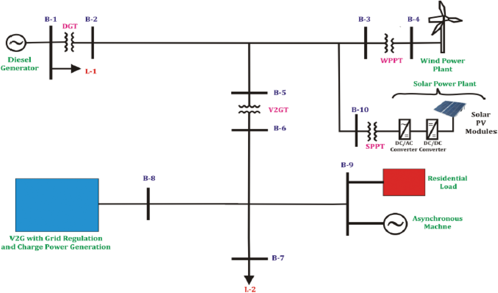
Figure 1: Schematic diagram of the designed microgrid with V2G interfacing
The diesel generator maintains a balance between the amount of energy consumed and the amount of energy generated. The rotor speed of its synchronous unit can be used to calculate grid frequency deviation. It is planned to build a diesel generator with a rated capacity of 15 MW, a 60 Hz frequency, and a 25 kV output voltage stage. A 3-phase synchronous machine modeled on the dq rotor reference frame is used to build a diesel generator. The windings of the stator are bound to an internal neutral point in a star configuration. The transfer feature (Hc) of the diesel engine governor system is planned using the following relationship:
Actuator transfer function (Ha) is given by the following relation:
Here, regulator time constants T1, T2, and T3 are considered, respectively, as 0.01, 0.02, and 0.2. Actuator time constants T4, T5, and T6 are taken to be equal to 0.25, 0.009, and 0.0384, respectively. Engine time delay (Td) equals 0.024. The initial value of mechanical power is taken as 0.1361. An IEEE type-1 synchronous machine voltage regulator is combined with an exciter to realize the excitation system of the diesel generator.
The architecture of the microgrid takes into account two RE power plants. The first is a solar PV farm, which generates energy proportional to three factors, one of which is the scale of the solar PV farm's coverage area. These solar PV panels’ efficiency and solar irradiance data are used. Second, to generate electricity, a basic model design of a wind power plant is used. This is made to follow a straight line with wind speed. When the wind speed reaches a nominal magnitude, the wind power plant produces nominal power. When the wind speed reaches the maximum allowable value, the wind farm effectively trips the grid. This will be turned off before the wind returns to its normal strength. The wind farm and PV plant are described in more detail below.
a. Solar PV Plant
A solar photovoltaic plant with an output power of 8 MW is designed to produce energy proportional to three factors: the size of the PV farm's coverage area, solar panel performance, and irradiance data. Irradiance is simulated to mimic real-time fluctuations of solar insolation. At 12 h, partial shading is also simulated for a time period of 300 s. PV plates with a total area of 80,000 m2 are considered. For this analysis, a PV plate efficiency of 10% is taken into account. PV farms produce power at 60 Hz at 25 kV and are connected to the grid directly.
b. Wind Power Plant
The simplified wind farm model is shown here, which generates power using a linear relationship between nominal wind speed and nominal power and trips from the grid when the wind speed exceeds its maximum value. The power is set to 1 p.u. when the wind speed is between the nominal and maximum values. The wind farm has a 4.5 MW power rating. The overall wind speed is 15 m/s2 and the nominal wind speed is 13.5 m/s2. The wind generator produces electricity at a voltage of 575 volts and a frequency of 60 Hz.
A generic aggregation of electric vehicles is modeled by V2G. The model has five different profiles, each of which can be changed under the mask by adjusting the plug and state of charge lookup tables. The number of vehicles that will follow each type of profile may be set by the user. The user can also choose the rated volume, rated power, and efficiency of the power converter. Each car has a power output of 40 kW. As a result, the total power rating of V2G is 4 MW. The V2G serves two purposes. During the day, it regulates the charge of the battery integrated with it and uses available power to regulate grid parameters. This arrangement implements five different types of car-user profiles:
Profile #1: People going to work with a possibility to and charges cars at work (Total number of cars: 35).
Profile #2: People going to work and charge cars at work but has longer ride period (Total number of cars: 25).
Profile #3: People going to work and do not charge cars at work (Total number of cars: 10).
Profile #4: People staying at home (Total number of cars: 20).
Profile #5: People working on a night shift (Total number of cars: 10).
It provides the minimum and maximum, charging and discharging rate of BEV.
Discharging mode:
Charging mode:
where
where,
A brief description of V2G technology used for the study illustrating the operational framework is shown in Fig. 2. An aggregator is used to control the frequency of the PHEVs. The fleet of vehicles is being continuously monitored by the V2G aggregator monitors integrated into the network of the power grid. The aggregate profile depends on the number of vehicles with V2G capability. The power includes the available power and energy which can be fed to the fleet of vehicles. The aggregator is capable of receiving signals/commands from the operator, which are forwarded to the fleet of vehicles, and accordingly, the regulation capability of the PHEV fleet is estimated and decided upon an optimal bidding strategy. The aggregator will decide and direct a particular PHEV for participation in the frequency control using the bidirectional energy exchange. Real-time frequency and battery state of charge are used by the V2G controller to take decisions for the battery management system (BMS). The V2G controller also controls the charger/discharger block/sequence. The BMS also monitors the battery's healthy state of charge (SOC). Detailed expressions of the controls used for the study are available in [52].
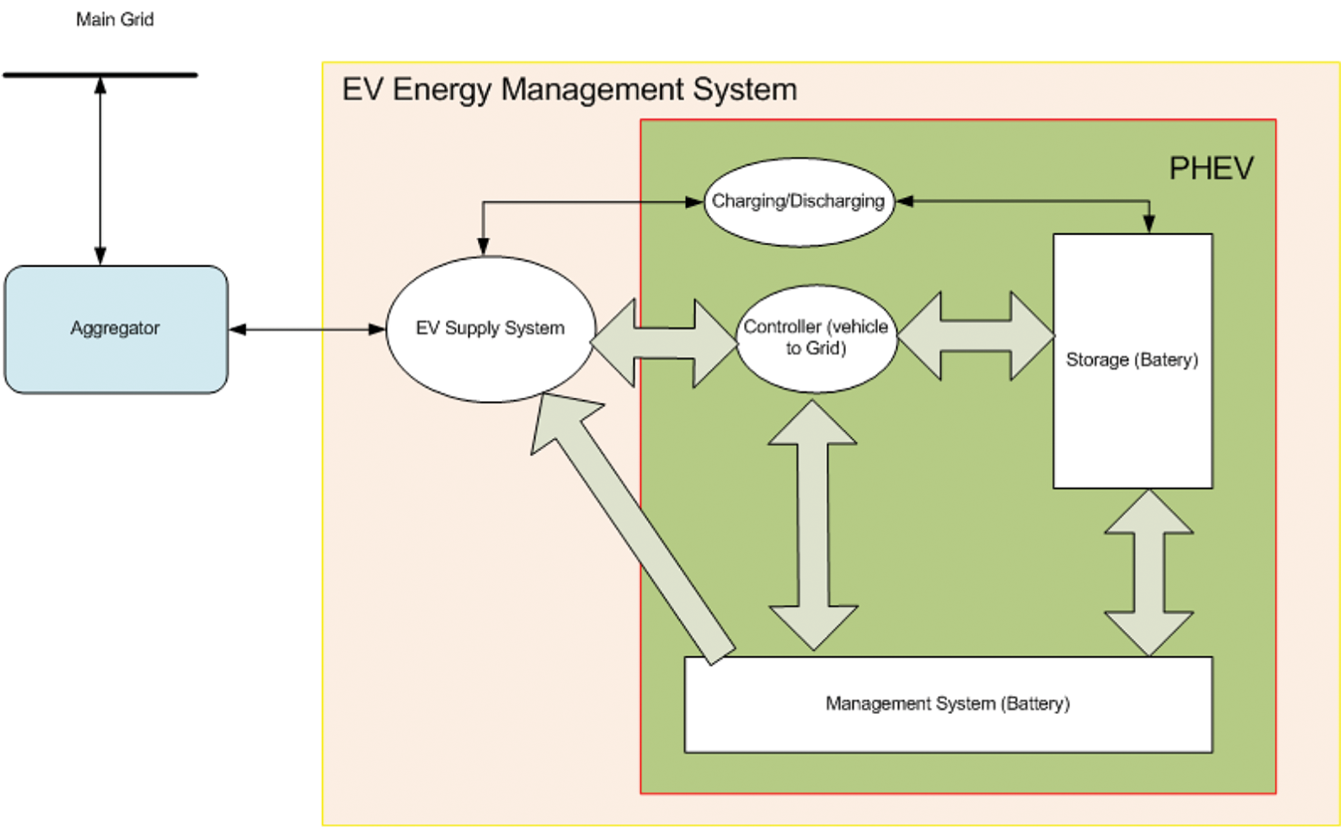
Figure 2: Framework of vehicle to grid (V2G) operation
A load is made up of residential loads and an asynchronous machine, which is used to simulate the effects of an industrial inductive load on a microgrid. These loads may have their own nature, such as ventilation systems. Residential loads adopt the consumption profile at a power factor of 0.95. The total capacity of the load considered is 10 MW. The ASM is controlled by a square relationship between the rotor speed and the mechanical torque. ASM is switched on at the moment of 3 h after the start of the simulation. The ASM is rated at 0.15 MW with a frequency of 60 Hz. Furthermore, loads L1 and L2 used in the network are rated at 1 kW each.
For a total of 24 h, the model will be simulated. Solar radiation intensity follows a normal distribution range, with maximum intensity occurring in the middle of the day. Wind intensity varies greatly during the day, with various peaks and small amplitude bursts. Residential load is simulated to follow a typical pattern that is close to a typical household load consumption pattern. Consumption is low during the day and rises to a peak during the evening hours. During the night hours, this gradually decreases. The following three conditions would have an effect on grid parameters during the day:
• The kick-off of ASM was early in the third hour.
• You will notice partial shading at noon, which affects the generation of solar power.
• A wind farm trips every 22 h when the wind exceeds the maximum allowed wind speed.
The main objective of the study is to balance the power in the system to minimize the variations in the system parameters such as frequency and voltage and keep the power import from the utility network to a minimum. The power balance requirement is assessed by the difference between generation by the RE generators, asynchronous machines, and demand by the non-EV loads and the EV load as described by Eq. (9). On bus B1 of the test system, it is decided to import or export power from/to the main utility grid depending on whether the power balance is positive or negative.
where, Pwind, Ppv, Pgrid, PV2G, Pbattc and Pasm represent the power from wind, solar, main grid, PHEV discharge, battery energy storage system and asynchronous machine respectively. Pres, PG2V and Pbattd represents residential, commercial, PEV charging demand and the BESS demand.
Considering the main objective is to minimize the power exchange with the utility grid and variations in the system parameters, it is focused on minimizing the cost and simultaneously providing high quality power to the customers. The objective function in terms of the cost is defined below:
where, TC is the summation of PV panel (TCPV), diesel generator (TCD), asynchronous machine (TASM), inverter (TCinv), and battery storage (TCB) and installation of HPEV (ICHPEV) costs. Following constraints are considered for present study [2,53]:
• SOC limits
• Charging/discharging rate limits
• Duration of presence in the parking lot
• The number of switching between charging and discharging
The V2G battery life period is used to determine the maximum number of switching between charging and discharging.
• The battery energy limit
The following are advantages of the use of proposed V2G and microgrid concepts:
• Designed V2G and microgrid concepts improve the performance of the electricity grid in terms of increased efficiency, stability, and reliability.
• A V2G-capable vehicle offers reactive power support, active power regulation, tracking of variable RE sources, load balancing, and current harmonic filtering.
• The designed V2G and microgrid effectively control the voltage and frequency. It also provides the spinning reserve, which helps to maintain an uninterrupted power supply.
• The Energy V2G batteries are effectively utilized to mitigate the variations due to the intermittent nature of RE power and variations in demand.
• It effectively handles the uncertainties of the RE generation. During a sudden increase in RE generation, power is absorbed by the battery of V2G, and conversely, when RE generation suddenly decreases, power is supplied by the battery of V2G. Similarly, a sudden change in demand for electrical power will be compensated for by the bidirectional exchange of power between the grid and the battery of V2G.
A designed model of the microgrid with V2G is simulated for analysis of the power profile, including the profile of both generation and consumption, for a whole day of 24 h. The contribution of every generation plant and the effect of the V2G system are regulated considering the peak demands and generation.
This section details the simulation results of variations in the system's parameters such as frequency, current, voltage, active power and reactive power associated with the conventional diesel generator, solar PV plant, wind power plant, and battery charging stations. Further, the results of the state of charge of all the five car pools are also discussed in this section. Analysis of the results is achieved with the aim of showing the effectiveness of the proposed design of the micro grid interfaced with V2G. Results of parameters associated with phase-A are discussed in this section. Similar results were also obtained for phases-B and C.
3.1 Parameters Associated to Diesel Generator
This section details the results of parameters pertaining to the conventional diesel generator. A diesel generator produces power according to the rotor speed because the governor rotor is directly coupled with the generator shaft. The normal rotor speed is kept at 1 m/s whereas the rotor is changed between 2.65 and 2.7 h, 11 to 11.4 h, and 21.8 to 22.4 h to regulate the power in the grid due to variations in the operating conditions due to the different profiles considered in the study. Hence, a diesel generator will be utilized to mitigate the variability of the generation load balance by variations in the rotor speed as shown in Fig. 3.
Voltage associated with phase-A recorded on Bus B1 of the test system is described in Fig. 4a. There are variations in the voltage for five time durations. Fig. 4 shows the high time resolution plots of voltage at which high variations are observed.
Fig. 4b details that the maximum voltage deviation of 2.5% is observed between the time intervals of 2.65 and 2.7 h. Fig. 4c details that the voltage sag of magnitude 0.024% is observed between the time intervals of 7 and 7.6 h. Fig. 4d details that transient components with magnitude amplitude deviations of 0.245% and 0.392% are observed in the time intervals of 11.05 to 11.15 h and 11.25 to 11.35 h, respectively. Fig. 4e illustrates that the voltage sags of magnitude 0.098% and 0.061% are observed between the time intervals of 17.6 to 18.2 h and 18.8 to 19.5 h, respectively. Fig. 4f details that transient components with amplitude deviations of 0.735% and 0.245% are observed in the time intervals of 21.7 to 22 h and 22.25 to 22.40 h, respectively.
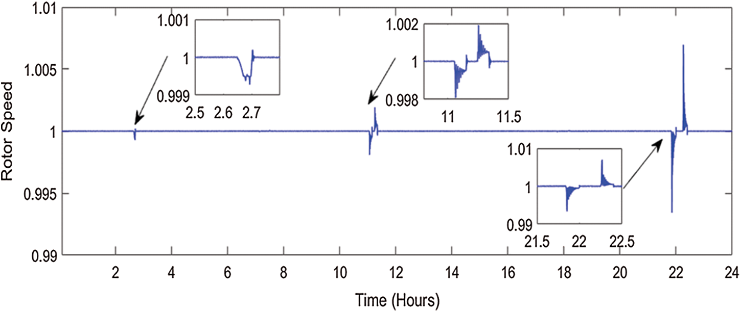
Figure 3: Rotor speed of diesel generator governor
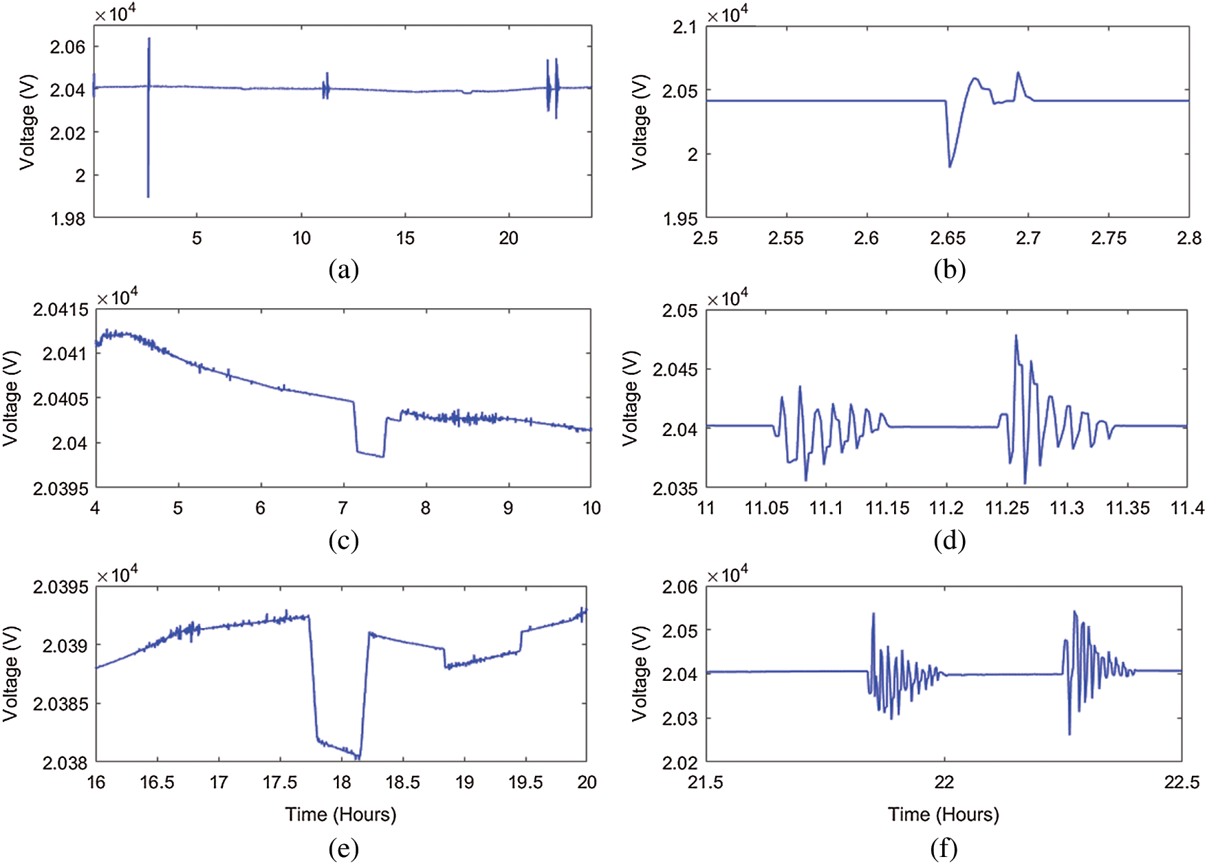
Figure 4: Voltage measured on the bus of source (diesel generator) (a) voltage profile for 24 h (b) high time resolution plot between 2.5 to 2.8 h (c) high time resolution plot between 3 to 10 h (d) high time resolution plot between 11 to 11.4 h (e) high time resolution plot between 16 to 20 h (f) high time resolution plot between 21.5 to 22.5 h
Current supplied by the diesel generator to the grid network is shown in Fig. 5. The magnitude of current is increased and decreased according to the generation of power from the wind and solar power plants as well as power exchange with the V2G system. Hence, different spikes and a reduced magnitude of the current are observed in this plot.
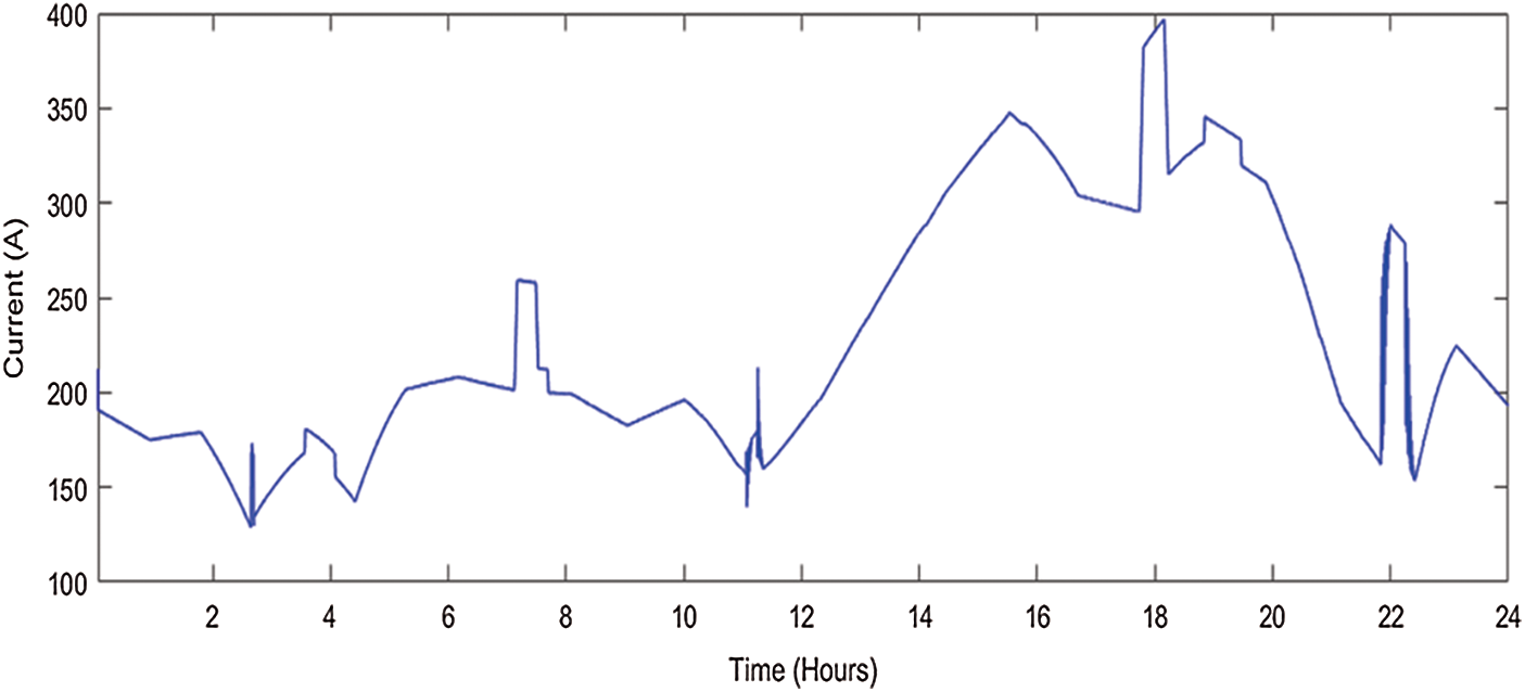
Figure 5: Profile of current measured on the bus of source (diesel generator) for 24 h
The active power supplied by the diesel generator to the grid network is shown in Fig. 6. The magnitude of power is increased and decreased according to the generation of power from the wind and solar power plants as well as power exchange with the V2G system. Hence, different spikes and a reduced magnitude of the power are observed in this plot.
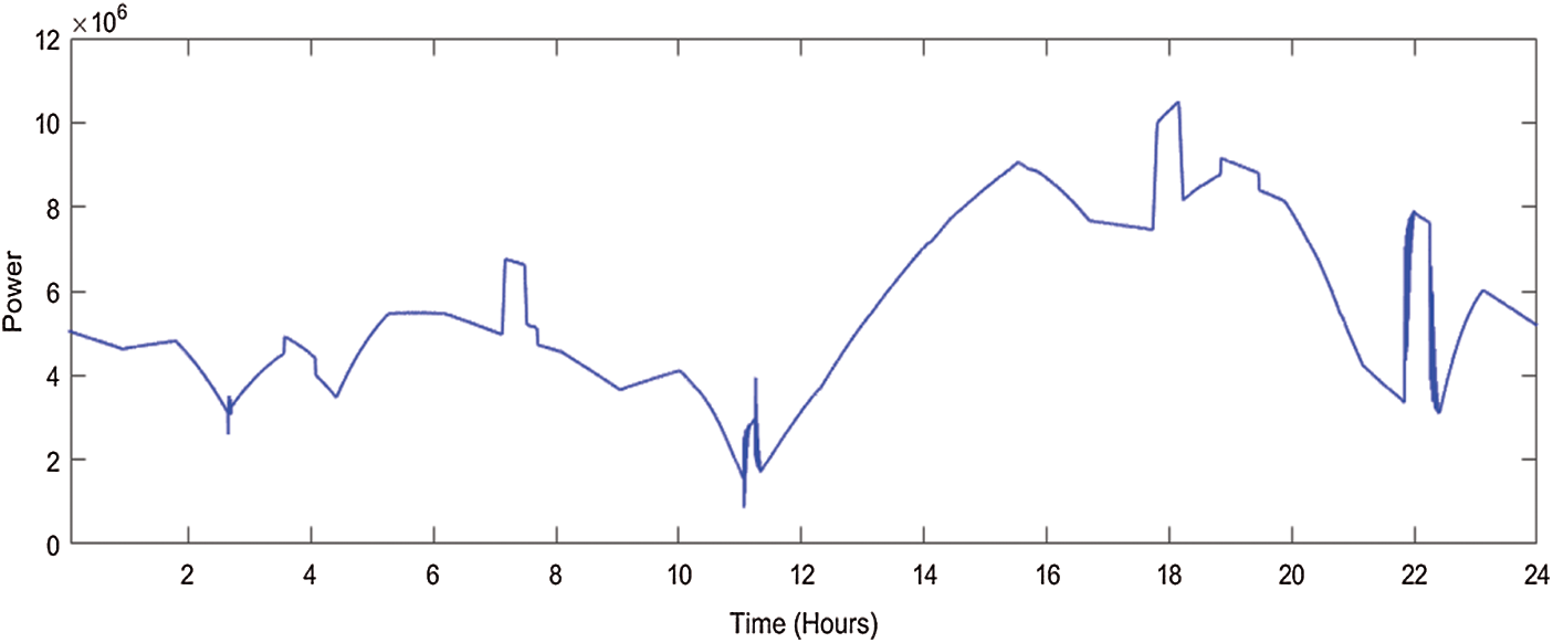
Figure 6: Profile of power measured on the bus of source (diesel generator) for 24 h
The reactive power supplied by the diesel generator to the grid network is shown in Fig. 7. The magnitude of reactive power is increased and decreased according to the generation of reactive power from the wind and solar power plants as well as reactive power exchange with the V2G system. Hence, different spikes and a reduced magnitude of the reactive power are observed in this plot. Sharp magnitude peaks indicate the reactive power exchange with the generator and microgrid.
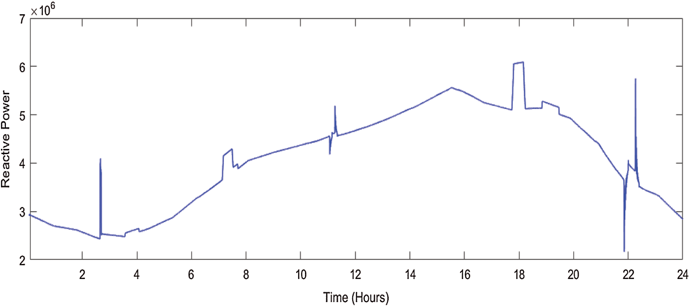
Figure 7: Profile of reactive power measured on the bus of source (diesel generator) for 24 h
3.2 Parameters Associated to Wind Power Plant
This section details the results of parameters recorded on the bus B4 of the test system and variations in the input wind speed to the wind turbine. Variations in the wind speed for a period of 24 h are considered inputs to the wind turbine for the generation of power from the wind power plant. This is illustrated in Fig. 8. From this figure, it is observed that the nominal wind speed is 9 m/s2 and that wind speeds vary between 7 and 15 m/s2 at different moments of time. This variable wind speed will generate variable power, which simulates a real-time scenario of wind power generation variations.
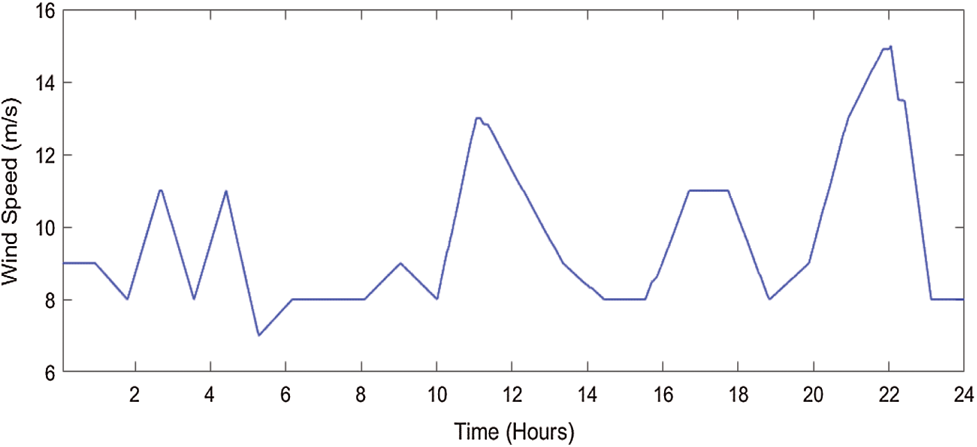
Figure 8: Wind speed variations for 24 h
Voltage associated with phase-A recorded on Bus B4 of the test system is described in Fig. 9a. There are variations in the voltage for seven time durations. Fig. 9 shows the high time resolution plots of voltage at which variations are observed.
Fig. 9b details that the maximum voltage deviation of 4.78% is observed between the time intervals of 2.65 and 2.7 h. Fig. 9c details that the voltage sag of magnitude 0.217% is observed between the time intervals of 3.5 and 4.1 h. Fig. 9c details that the voltage sag of magnitude 1.087% is observed between the time intervals of 7.1 and 7.8 h. Fig. 9d details those transient components with magnitude amplitude deviations of 0.783% and 0.652% are observed in the time intervals of 11.05 to 11.15 h and 11.25 to 11.35 h, respectively. Fig. 9e illustrates that voltage sags of magnitudes of 0.761% and 0.217% are observed between the time intervals of 17.6 to 18.2 h and 18.8 to 19.5 h, respectively. Fig. 9f details those transient components with amplitude deviations of 1.52% and 1.304% are observed in the time intervals of 21.7 to 22 h and 22.25 to 22.40 h, respectively.
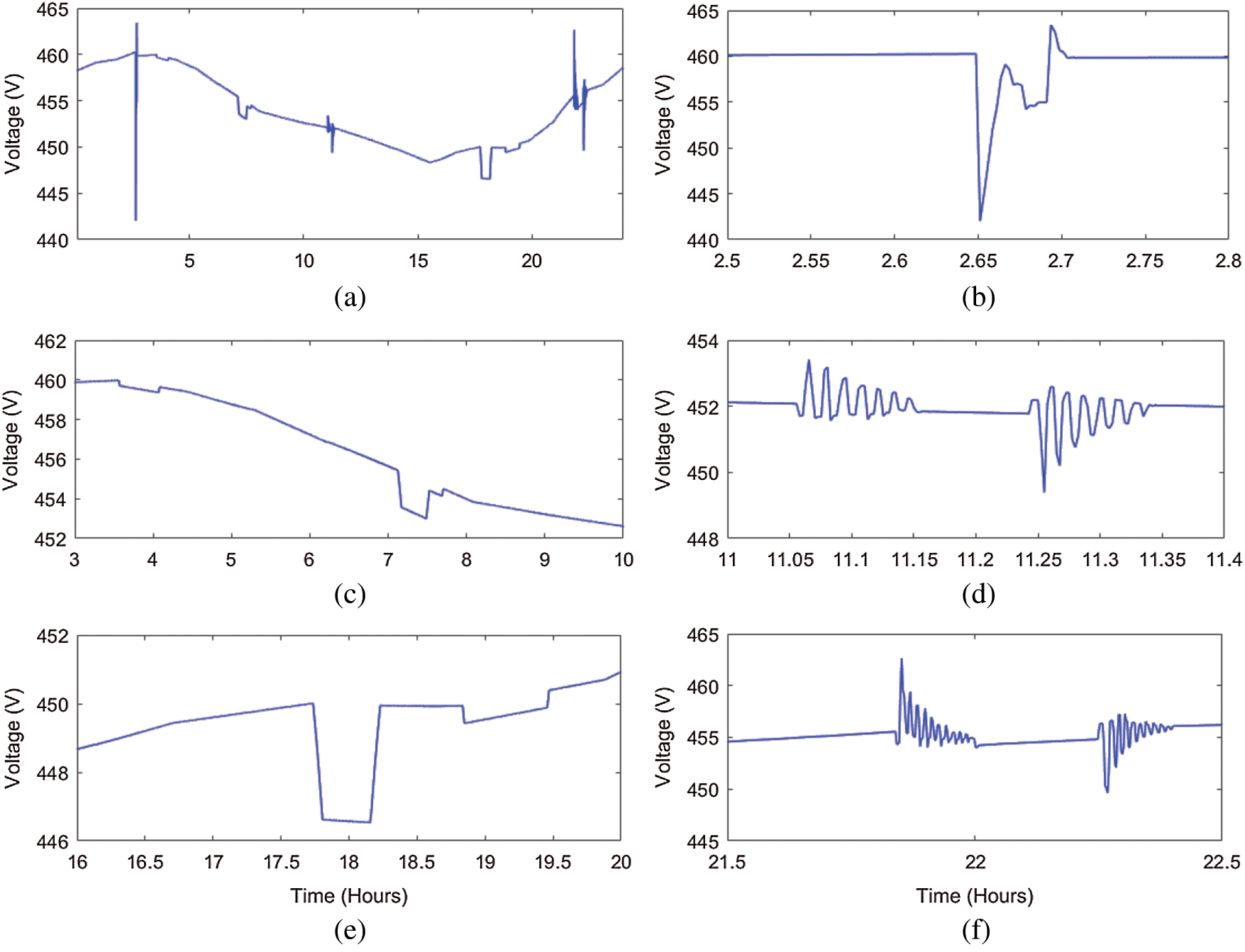
Figure 9: Voltage measured on the bus of wind power plant (a) voltage profile for 24 h (b) high time resolution plot between 2.5 to 2.8 h (c) high time resolution plot between 3 to 10 h (d) high time resolution plot between 11 to 11.4 h (e) high time resolution plot between 16 to 20 h (f) high time resolution plot between 21.5 to 22.5 h
The current supplied by the wind generator to the grid network is shown in Fig. 10. The magnitude of the current is increased and decreased according to the wind speed variations. If the wind speed increases, the current supplied by the wind generator to the utility grid also increases. Further, if the wind speed decreases, the current supplied by the wind generator to the utility grid also decreases. Hence, the current supplied by the wind generator will depend on variations in wind speed.
The power supplied by the wind generator to the grid network is shown in Fig. 11. The magnitude of power is increased and decreased according to the wind speed variations. If the wind speed increases, the power supplied by the wind generator to the utility grid will also increase. Further, if the wind speed decreases, the power supplied by the wind generator to the utility grid also decreases. Hence, the power supplied by the wind generator will depend on the wind speed variations.
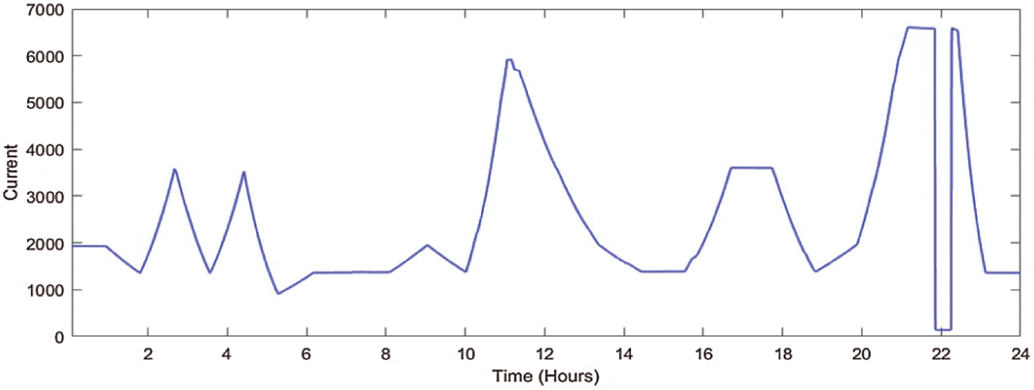
Figure 10: Profile of current measured on the bus of wind power plant for 24 h
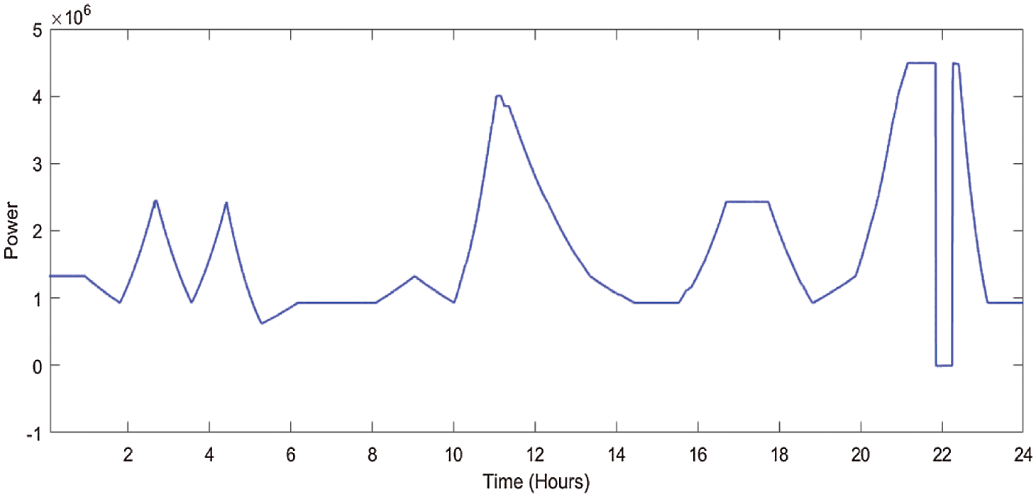
Figure 11: Profile of power measured on the bus of wind power plant for 24 h
The reactive power exchange by the wind generator to the grid network is shown in Fig. 12. Magnitude of reactive power is changed at three time intervals between 2.6 to 2.75 h, 11 to 11.4 h and 21.8 to 22.4 h. This helps is regulating the variations in the system parameters specifically the voltage of microgrid.
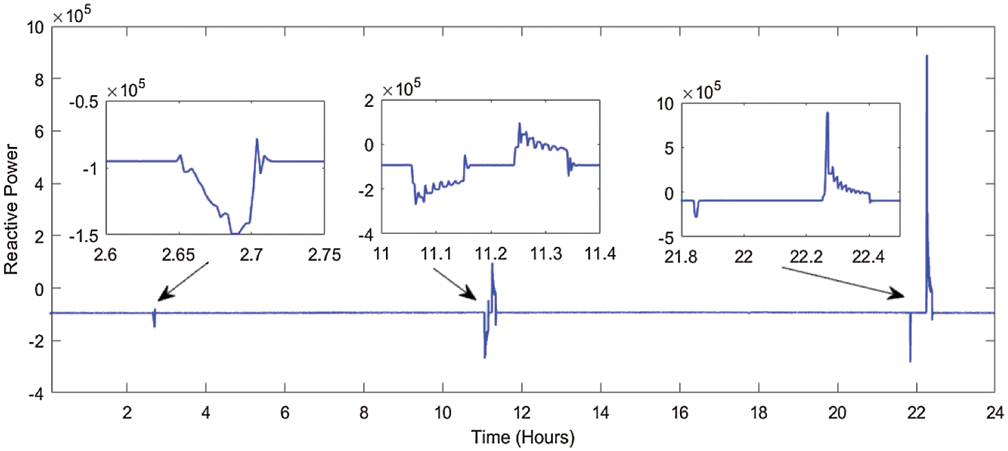
Figure 12: Profile of reactive power measured on the bus of wind power plant for 24 h
3.3 Parameters Associated to Solar PV Power Plant
This section details the results of parameters recorded on the bus B10 of the test system and variations in the input solar insolation. Variations in the solar irradiance for a period of 24 h considered as input to the solar PV plates for generating power from the solar PV plant are illustrated in Fig. 13. It is observed that the maximum irradiance is 500 (w/m2). Partial shading is also simulated for a period of 300 s at 12 h, which is indicated by a decreased value of the solar irradiance. This variable solar irradiance will generate variable power, which simulates the real-time scenario of solar power generation variations. Solar irradiance starts rising at 6 h and decreases to zero after 18 h.
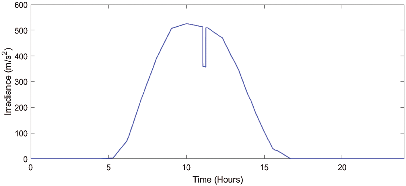
Figure 13: Variations of solar irradiance for a period of 24 h
Voltage associated with phase-A recorded on Bus B10 of the test system is shown in Fig. 14a. There are variations in the voltage for seven time durations. Fig. 14 shows the high time resolution plots of voltage at which variations are observed.
Fig. 14b details that the maximum voltage deviation of 4.0% is observed between the time intervals of 2.65 and 2.7 h. As shown in Fig. 14c, voltage sag of magnitude 0.04% is observed between the time intervals of 3.5 and 4.1 h. Fig. 14c details that the voltage sag of magnitude 0.5% is observed between the time intervals of 7.1 and 7.8 h. Fig. 14d details those transient components with magnitude amplitude deviations of 0.45% and 1.30% are observed in the time intervals of 11.05 to 11.15 h and 11.25 to 11.35 h, respectively. Fig. 14e shows that the voltage sags of magnitude 0.90% and 0.50% are observed between the time intervals of 17.6 to 18.2 h and 18.8 to 19.5 h, respectively. Fig. 14f details those transient components with amplitude deviations of 1.50% and 1.75% are observed in the time intervals of 21.7 to 22 h and 22.25 to 22.40 h, respectively.
The current supplied by the solar PV generator to the grid network is shown in Fig. 15. The magnitude of the current is increased and decreased according to the irradiance variations. If the irradiance level increases, then the current supplied by the solar PV generator to the utility grid will also increase. Further, if the irradiance decreases, then the current supplied by the solar PV generator to the utility grid also decreases. Hence, the current supplied by the solar PV generator will depend on the variations in the irradiance. Also, the current decreases after the partial shading on the solar PV plates. In general, the nature of the current curve is similar to that of irradiance.
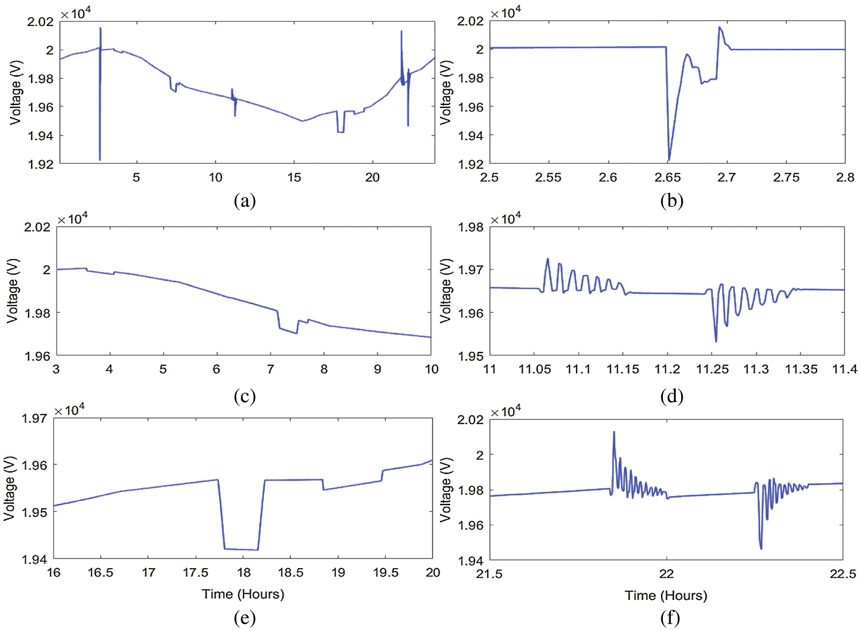
Figure 14: Voltage measured on the bus of solar PV power plant (a) voltage profile for 24 h (b) high time resolution plot between 2.5 to 2.8 h (c) high time resolution plot between 3 to 10 h (d) high time resolution plot between 11 to 11.4 h (e) high time resolution plot between 16 to 20 h (f) high time resolution plot between 21.5 to 22.5 h
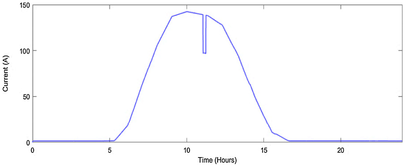
Figure 15: Profile of current measured on the bus of solar PV power plant for 24 h
The power supplied by the solar PV generator to the grid network is shown in Fig. 16. The magnitude of power generated is increased and decreased according to the irradiance variations. If the irradiance level increases, the power supplied by the solar PV generator to the utility grid also increases. Further, if the irradiance decreases, then the power supplied by the solar PV generator to the utility grid also decreases. Hence, the power supplied by the solar PV generator will depend on variations in the irradiance. Power output also decreases after the partial shading on the solar PV plates. In general, the nature of the power curve is similar to that of irradiance.
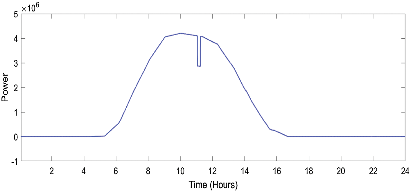
Figure 16: Profile of power measured on the bus of solar PV power plant for 24 h
The reactive power exchanged between the solar PV generator and the grid network is shown in Fig. 17. The magnitude of reactive power exchange between the solar PV generator and the microgrid network depends on the grid conditions. If there is excessive reactive power on the bus to which the solar PV generator is connected, then reactive power is absorbed by the PV plant. If there is a low level of reactive power at the bus of the solar PV generator, then the reactive power will be supplied by the solar PV generator. Reactive power exchange between the solar PV generator and the microgrid network takes place between 7 and 8 h, 10.8 to 11.4 h, and 21.5 to 22.8 h.
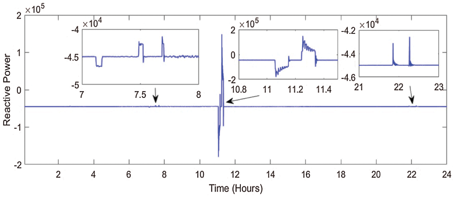
Figure 17: Profile of reactive power measured on the bus of solar PV power plant for 24 h
3.4 Parameters Associated to Consumer Load
This section details the results of parameters recorded on bus B9 of the test system associated with the consumer loads. Voltage associated with phase-A recorded on Bus B9 of the test system illustrated in Fig. 1 is shown in Fig. 18a. There are variations in the voltage for seven time durations. Fig. 18 shows the high time resolution plots of voltage at which variations are observed. Fig. 18b details that a maximum voltage deviation of 5.74% is observed between the time intervals of 2.65 and 2.7 h. Fig. 18c details that the voltage sag of magnitude 0.425% is observed between the time intervals of 3.5 and 4.1 h. Fig. 18c details that a voltage sag of magnitude 0.813% is observed between the time intervals of 7.1 and 7.8 h. Fig. 18d details transient components with magnitude amplitude deviations of 0.42% and 1.27%, which are observed in the time intervals of 11.05 to 11.15 h and 11.25 to 11.35 h, respectively. Voltage sags of 1.06% and 0.425%, respectively, are observed between the time intervals of 17.6 h to 18.2 h and 18.8 to 19.5 h, as shown in Fig. 18e. Fig. 18f details the transient components with amplitude deviations of 3.19% and 3.83%, which are observed in the time intervals of 21.7 to 22 h and 22.25 to 22.40 h, respectively.
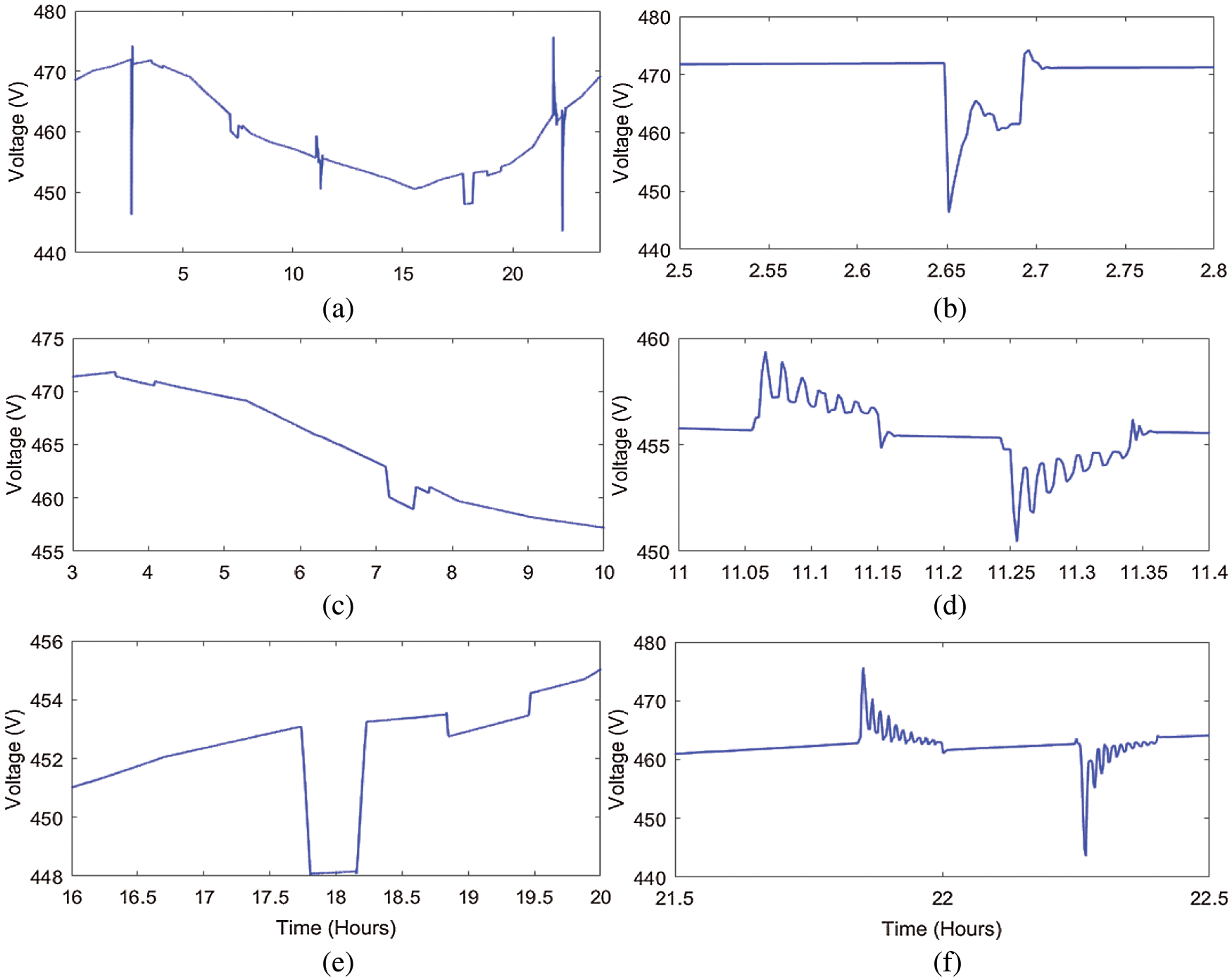
Figure 18: Voltage measured on the bus of consumer load (a) voltage profile for 24 h (b) high time resolution plot between 2.5 to 2.8 h (c) high time resolution plot between 3 to 10 h (d) high time resolution plot between 11 to 11.4 h (e) high time resolution plot between 16 to 20 h (f) high time resolution plot between 21.5 to 22.5 h
The current drawn by the load from the microgrid network is shown in Fig. 19. The magnitude of current is increased and decreased according to variations in the load demand. A minimum current of 8000 A and a maximum current of 16000 A are drawn from the grid. Further, local variations are observed when load demand varies. Sudden changes in load demand are observed at 2.6 to 2.7 h, 10.4 to 10.5 h, 17.5 to 18.2 h, and 20 to 22.5 h. Variations in the load demand are mitigated by the current balance using the V2G.
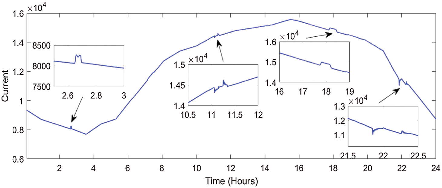
Figure 19: Profile of current measured on the bus of consumer load for 24 h
The power drawn by the load from the microgrid network is shown in Fig. 20. The magnitude of power is increased and decreased according to the variations in the load demand. Power drawn from the microgrid by the load varies from 107 W to 5.5 × 10⁶ W. Sudden changes in load demand are observed at 2.6 to 2.7 h, 10.4 to 10.5 h, 17.5 to 18.2 h, and 20 to 22.5 h. Variations in the load demand have been mitigated by the current balance using the V2G.
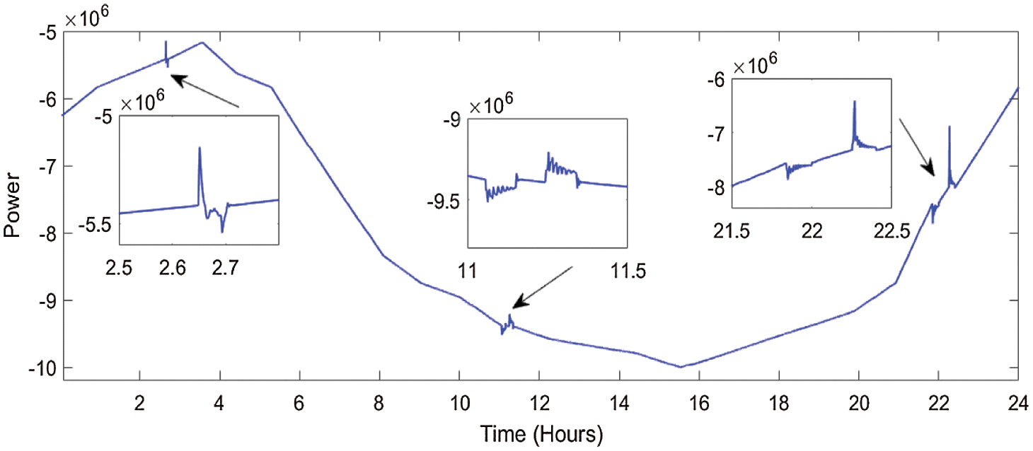
Figure 20: Profile of power measured on the bus of consumer load for 24 h
The reactive power drawn by the load from the microgrid network is shown in Fig. 21. The magnitude of reactive power is increased and decreased according to the variations in the reactive power demand of the load. Reactive power drawn from the microgrid by the load varies from 4 × 10⁶ W to 0.5 × 10⁶ W. Sudden changes in reactive power demand load are observed at 2.6 to 2.7 h, 11 to 11.4 h, and 21.5 to 22.8 h.
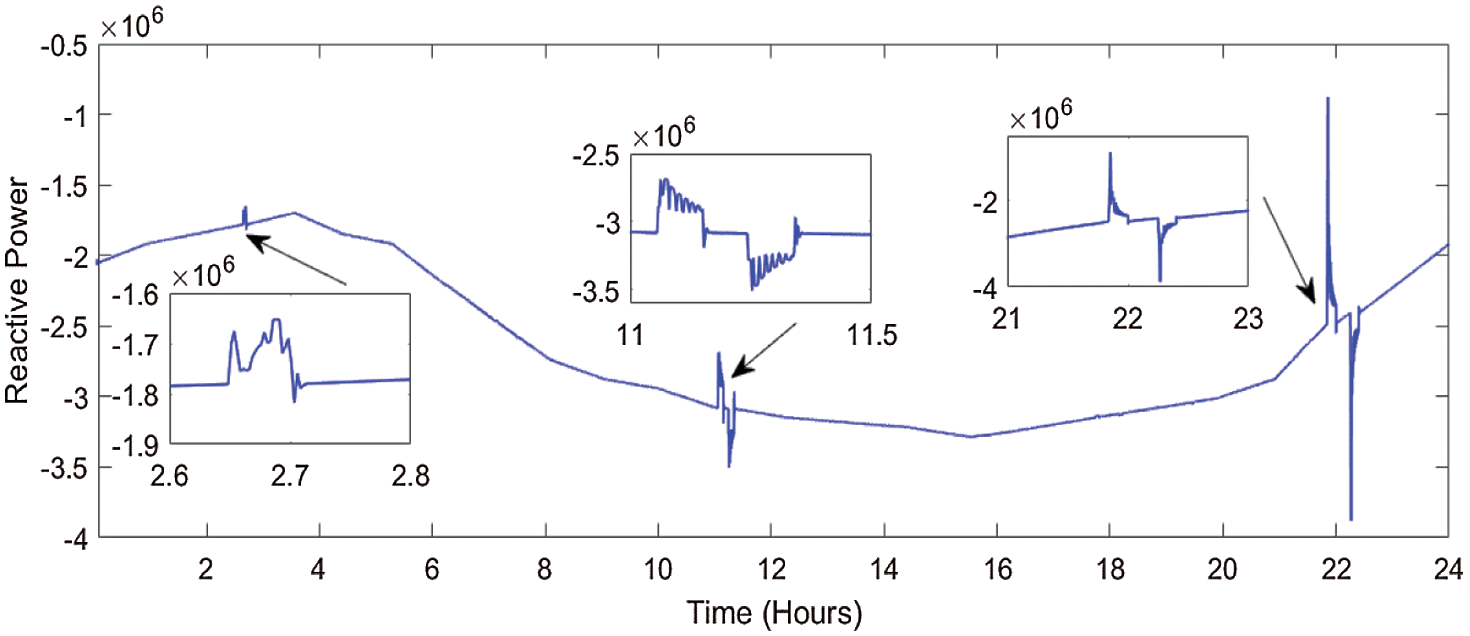
Figure 21: Profile of reactive power measured on the bus of consumer load for 24 h
3.5 Parameters for Asynchronous Machine
This section details the results of parameters associated with the asynchronous machine and recorded on bus B9 of the test system. Fig. 22a depicts the voltage associated with phase-A recorded on the test's bus B9. There are variations in the voltage for seven time durations. Fig. 22 shows the high time resolution plots of voltage at which variations are observed.
Fig. 22b details that a maximum voltage deviation of 5.72% is observed between the time intervals of 2.65 and 2.7 h. Fig. 22c details that the voltage sag of magnitude 0.212% is observed between the time intervals of 3.5 and 4.1 h. Fig. 22c details that the voltage sag of magnitude 1.063% is observed between time intervals of 7.1 and 7.8 h. Fig. 22d details those transient components with magnitude amplitude deviations of 1.48% and 0.638% are observed in the time intervals of 11.05 to 11.15 h and 11.25 to 11.35 h, respectively. Fig. 22e illustrates that the voltage sags of magnitude 0.638% and 0.425% are observed between time intervals of 17.6 to 18.2 h and 18.8 to 19.5 h, respectively. Fig. 22f details the transient components with amplitude deviations of 3.21% and 3.82%, which are observed in the time intervals of 21.7 to 22 h and 22.25 to 22.40 h, respectively.
An asynchronous machine load of 0.16 MVA is switched on every 3 h. The current drawn by the ASM from the grid is described in Fig. 23. From this figure, it is observed that the heavy current equals 2400 A is drawn at the moment of switching on the ASM, which indicates the inrush current. Subsequently, a constant current of 250 A is drawn. Further, variations in the current are also observed at 11 to 11:40 h and 21.8 to 22.4 h. These variations are observed according to power exchange with V2G.
An ASM load of 0.16 MVA is switched on for 3 h. Active power drawn by the ASM from the grid is shown in Fig. 24. From this figure, it is observed that heavy active power is drawn at the moment of switching on the ASM, which is due to inrush current. Subsequently, the constant active power of 0.15 MW is consumed by the ASM. Further, variations in the active power are also observed at 11 to 11:40 h and 21.8 to 22.4 h. These variations are observed according to power exchange with V2G.
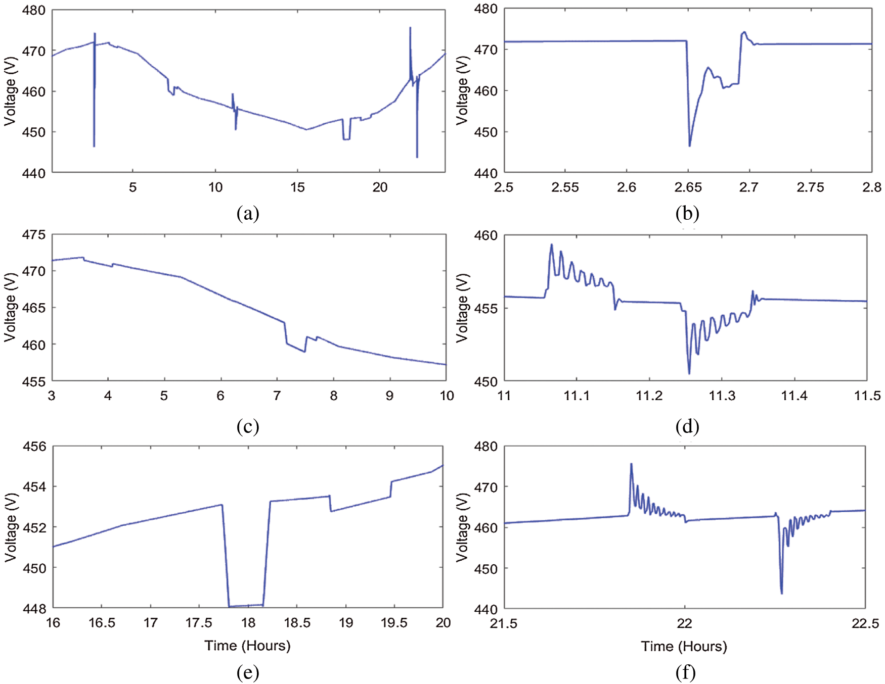
Figure 22: Voltage measured on the bus of asynchronous machine (a) voltage profile for 24 h (b) high time resolution plot between 2.5 to 2.8 h (c) high time resolution plot between 3 to 10 h (d) high time resolution plot between 11 to 11.4 h (e) high time resolution plot between 16 to 20 h (f) high time resolution plot between 21.5 to 22.5 h
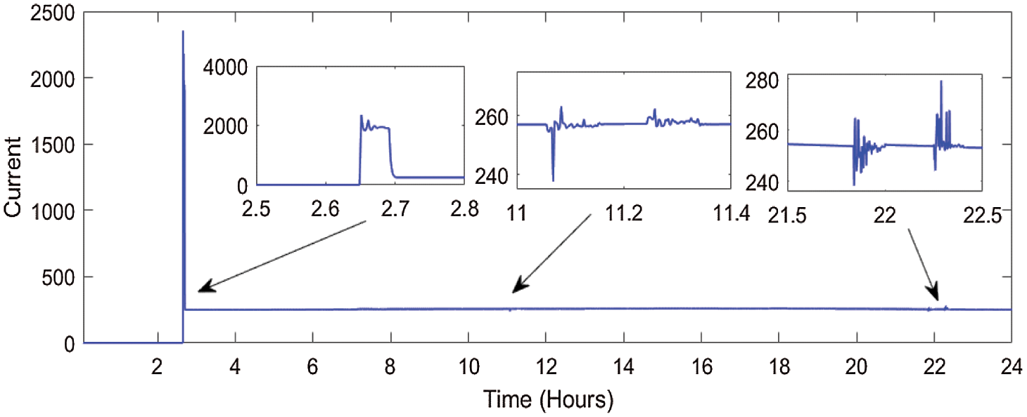
Figure 23: Profile of current measured on the bus of asynchronous machine for 24 h
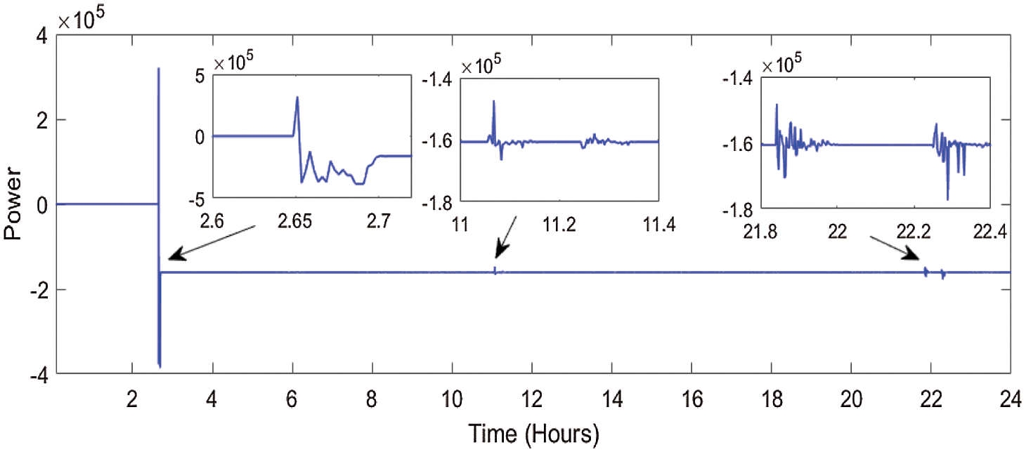
Figure 24: Profile of power measured on the bus of asynchronous machine for 24 h
An ASM load of 0.16 MVA is switched on for 3 h. Reactive power drawn by the ASM from the grid is shown in Fig. 25. It is observed that heavy reactive power is drawn at the moment of switching on the ASM, which is due to inrush current. Subsequently, constant reactive power of 0.2 MVAR is consumed by the ASM. Further, variations in the reactive power are also observed from 11 a.m. to 11:40 a.m. and from 21.8 a.m. to 22.4 a.m. These variations are observed according to reactive power exchange with V2G.
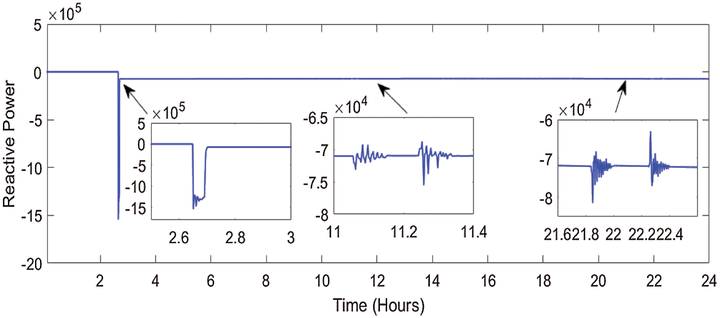
Figure 25: Profile of reactive power measured on the bus of asynchronous machine for 24 h
This section details the results of the parameters for V2G for regulation. Voltage associated with phase-A recorded on the voltage regulation unit of V2G connected to the test system's Bus B8 is depicted in Fig. 26a. There are variations in the voltage for seven time durations. Fig. 26 shows the high time resolution plots of voltage at which variations are observed.
Fig. 26b details that the maximum voltage deviation of 5.74% is observed between the time intervals of 2.65 and 2.7 h. Fig. 26c details that a voltage sag of magnitude 0.212% is observed between the time intervals of 3.5 and 4.1 h. As illustrated in Fig. 26c, voltage sag of magnitude 0.957% is observed between the time intervals of 7.1 and 7.8 h. Fig. 26d shows the transient components with magnitude amplitude deviations of 0.425% and 1.276% observed in the time intervals 11.05 to 11.15 h and 11.25 to 11.35 h. Voltage sags of 1.17% and 0.425% are observed between the time intervals of 17.6 to 18.2 h and 18.8 to 19.5 h, respectively, as shown in Fig. 26e. Fig. 26f shows the transient components with amplitude deviations of 3.82% and 2.55% observed in the time intervals of 21.7 to 22 h and 22.25 to 22.40 h, respectively.
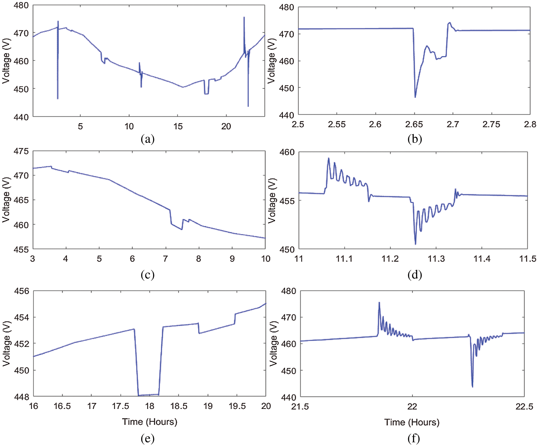
Figure 26: Voltage measured on the bus of voltage regulation unit of V2G (a) voltage profile for 24 h (b) high time resolution plot between 2.5 to 2.8 h (c) high time resolution plot between 3 to 10 h (d) high time resolution plot between 11 to 11.4 h (e) high time resolution plot between 16 to 20 h (f) high time resolution plot between 21.5 to 22.5 h
The current taken for regulation of the variations by the V2G is shown in Fig. 27. It is observed that the current is taken between 2.68 and 2.7 h. Further, current is also taken for a duration of between 11 and 11.4 h, with two high-magnitude peaks. Further, current is taken between the time durations of 21.8 to 22 h and 22.2 to 22.4 h with ripple magnitudes. Hence, currents used for the regulation of voltage variations are indicated by their high magnitude, while at all other times the magnitude of current is zero.
The power exchange for regulation of the variations by the V2G is shown in Fig. 28. It is observed that power is taken between 2.68 and 2.7 h. Further, the power is exchanged for the duration between 11 and 11.4 h with two high-magnitude peaks, where the first high-magnitude peak indicates that the power is taken by the V2G and the second magnitude indicates that the power is supplied by the V2G to mitigate the variations. Further, power is also exchanged between the time durations of 21.8 to 22 h and 22.2 to 22.4 h with ripple magnitudes. First, magnitude indicates the power taken by the V2G, and second, peak indicates the power supplied by the V2G to mitigate the variations in power. Hence, power used for the regulation of variations is shown to have a high magnitude, and at all other times, the magnitude of power is zero.
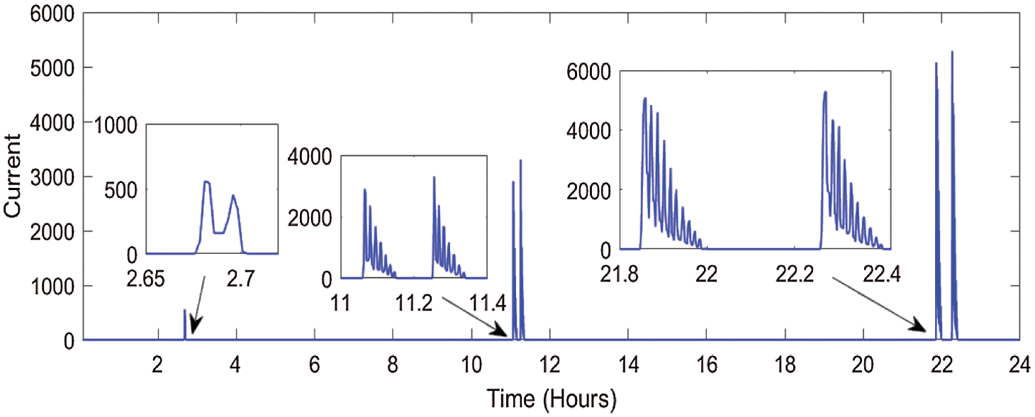
Figure 27: Profile of current measured on the bus of regulation for 24 h
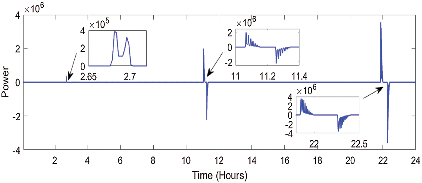
Figure 28: Profile of power measured on the bus of voltage regulation unit for V2G for 24 h
Reactive power exchange for regulation of variations by the V2G is shown in Fig. 29. It is observed that reactive power is exchanged between 2.68 and 2.7 h. Further, the reactive power is also exchanged for the duration between 11 and 11.4 h with two high-magnitude peaks. Further, reactive power is also exchanged between the time durations of 21.8 to 22 h and 22.2 to 22.4 h with ripple magnitudes. Hence, reactive power is used to improve the variations of voltage. At all other times, the magnitude of reactive power is zero.
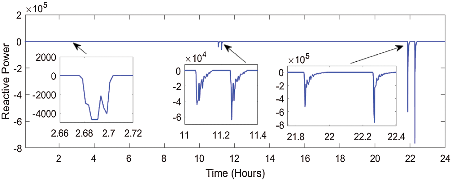
Figure 29: Profile of reactive power measured on the bus of voltage regulation unit for V2G for 24 h
3.7 Parameters for Charging the Batteries of Cars for V2G System
This section details the results of the parameters for V2G for the charging of car batteries. Voltage associated with phase-A recorded on the battery charging unit of V2G connected to Bus B8 of the test system is shown in Fig. 30a. There are variations in the voltage for seven time durations. High time resolution plots of voltage at which variations are observed are included in Figs. 30b–30f. Fig. 30b details that a maximum voltage deviation of 5.74% is observed between the time intervals of 2.65 and 2.7 h. Fig. 30c details that the voltage sag of magnitude 0.212% is observed between the time intervals of 3.5 and 4.1 h. Fig. 30c details that the voltage sag of magnitude 0.957% is observed between the time intervals of 7.1 and 7.8 h. The transient components with magnitude amplitude deviations of 0.425% and 1.276% observed in the time intervals 11.05 to 11.15 h and 11.25 to 11.35 h are detailed in Fig. 30d. Voltage sags of 1.17% and 0.425% are shown in Fig. 30e between the time intervals of 17.6 to 18.2 h and 18.8 to 19.5 h, in that order. Fig. 30f details those transient components with amplitude deviations of 3.82% and 2.55% are observed in the time intervals of 21.7 to 22 h and 22.25 to 22.40 h, respectively.
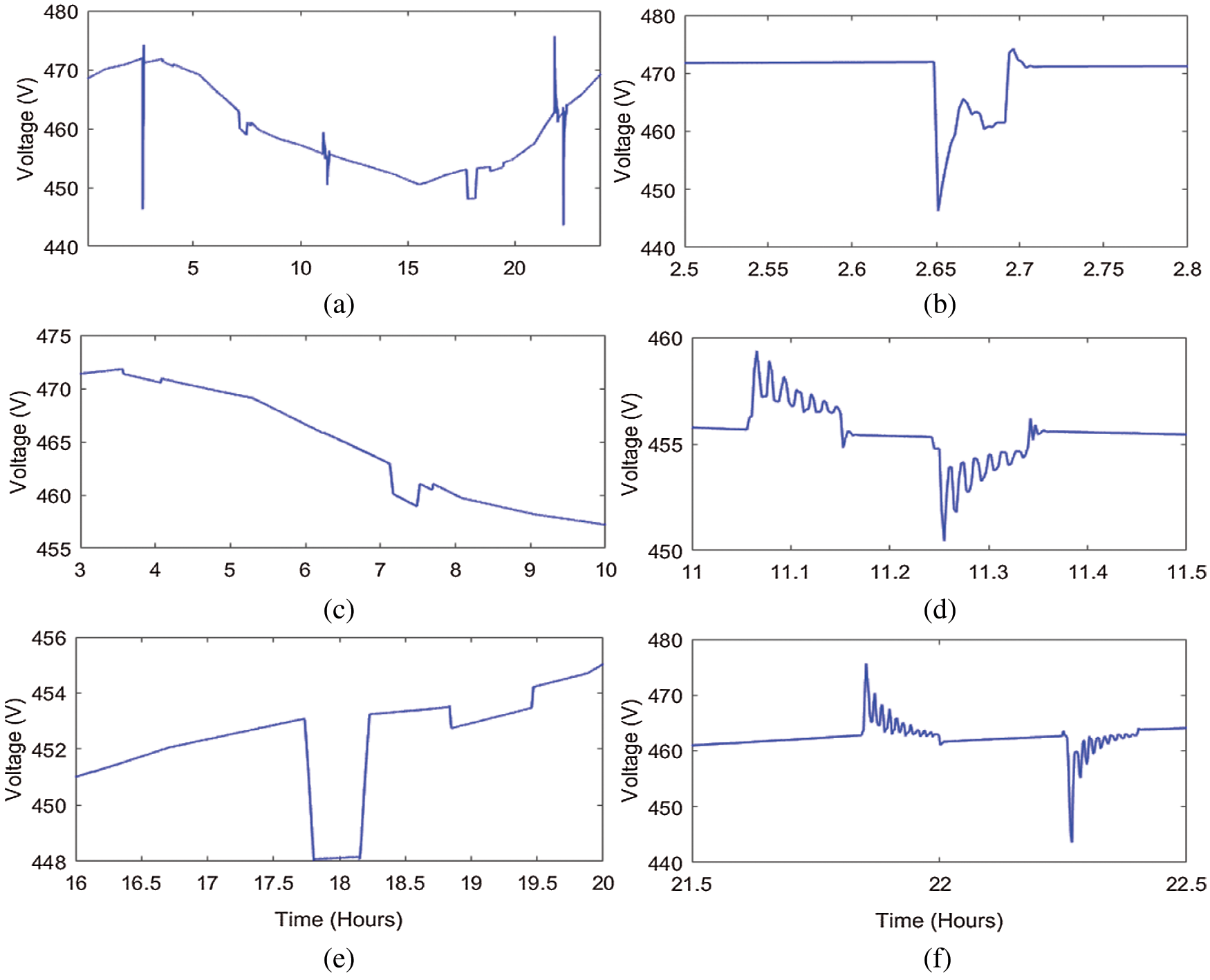
Figure 30: Voltage measured on the bus of battery charging unit of V2G (a) voltage profile for 24 h (b) high time resolution plot between 2.5 to 2.8 h (c) high time resolution plot between 3 to 10 h (d) high time resolution plot between 11 to 11.4 h (e) high time resolution plot between 16 to 20 h (f) high time resolution plot between 21.5 to 22.5 h
The following five profiles are considered for the study, where a possible period for charging the cars is also mentioned:
Profile #1: People going to work with a possibility to charge their cars at work (Total number of cars: 35). Cars are charged after reaching the office between 7 to 7:30 h.
Profile #2: People going to work and charges their cars at work and a longer ride period (Total number of cars: 25). Cars are charged after reaching the office between 7 to 7:45 h.
Profile #3: People going to work and do not charge their cars at work (Total number of cars: 10). Cars are charged at home either between 3:30 to 4 h or 19 to 19:30 h after reaching back to home.
Profile #4: People staying at home (Total number of cars: 20).
Profile #5: People working on a night shift (Total number of cars: 10). Cars are charged at home between 17:30 to 18:30 h.
The current profile measured on the bus for charging the cars of V2G is shown in Fig. 31. It is observed that there are four time durations where the car batteries draw power from the grid for charging purposes. Cars are charged between 3:30 and 4 h, 7 to 7:30 h, 17.6 to 18:20 h, and 19 to 19:30 h, which are indicated in Fig. 31 by the increased current draw from the grid.
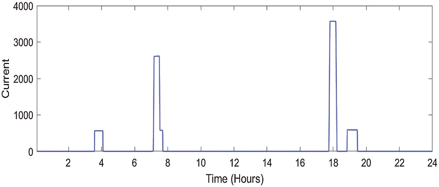
Figure 31: Profile of current measured on the bus of battery charging unit of V2G for 24 h
The power profile measured on the bus for charging the cars of V2G cars is shown in Fig. 32. It is observed that there are four time durations where car batteries draw power from the grid for charging purposes. Cars are charged between 3:30 and 4 h, 7 to 7:30 h, 17.6 to 18:20 h, and 19 to 19:30 h, which are shown in Fig. 32 by the decreased power. The power drawn from the grid is indicated as “negative”. Hence, batteries draw power from the grid for four time intervals as indicated above.
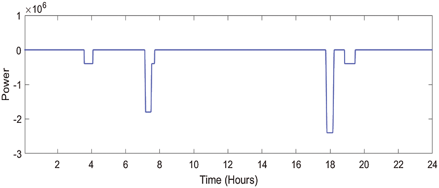
Figure 32: Profile of power measured on the bus of battery charging unit of V2G for 24 h
The reactive power profile measured on the bus for charging the cars of V2G cars is shown in Fig. 33. It is observed that there are four time durations where car batteries draw power from the grid for charging purposes. Cars are charged between 3:30 and 4 h, 7 to 7:30 h, 17.6 to 18:20 h, and 19 to 19:30 h. For these charging intervals, the reactive power exchange is indicated in Fig. 33. It is observed that at the moment of the start of charging batteries, the reactive power is supplied by the batteries, and at the moment of disconnecting the batteries from the charging station, the reactive power is drawn from the grid. Hence, reactive power exchange takes place only at the start and end of charging the batteries of cars.
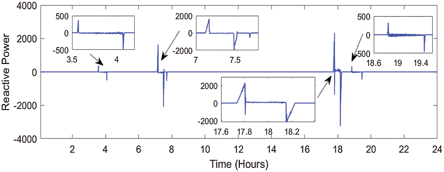
Figure 33: Profile of reactive power measured on the bus of battery charging unit of V2G for 24 h
The study was carried out for different scenarios of the five profiles used for the study, and maximum deviations in the various parameters are tabulated in Table 1. Time periods for all changes have been kept the same for all profiles. It is observed that the error in the measurement of voltage and frequency for the test grid for different scenarios of V2G vehicles is less than 5%. Hence, the proposed model of V2G and microgrid is not very sensitive to the change in the operating conditions and effectively operates in different operating scenarios.

3.8 Parameters for State of Charge of Batteries of V2G System
This section details the results of parameters for V2G for the state of charge of batteries in cars for all the five profiles considered for the study. The state of charge (SOC) of batteries for Profile #1 when people go to work with the possibility to charge their cars at work (Total number of cars: 35) over a period of 24 h is described in Fig. 34. It is observed that the SOC of the batteries decreases at the times when people go from their home to their work place in the morning hours. Similarly, the SOC also decreases when people return home from the workplace in the evening hours between 15:30 and 18 h. SOC increases during the period of the workplace when batteries are charged at the work place and become high above 90.
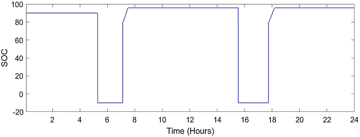
Figure 34: State of charge of batteries for Profile #1 when people going to work with a possibility to charge their car at work (Total number of cars: 35) over period of 24 h
The SOC of batteries for Profile #2 when people go to work with the option of charging their cars at work (Total number of cars: 25) over a 24 h period is depicted in Fig. 35. It is observed that the SOC of the batteries decreases at the times when people are on a long drive period between 4:30 and 7:30 a.m. while going from home to their workplace in the morning hours. Similarly, the SOC also decreases when people return home from the workplace in the evening hours between 15:30 and 19:00. SOC increases during the period of the workplace when batteries are charged at the workplace and becomes high above 90.
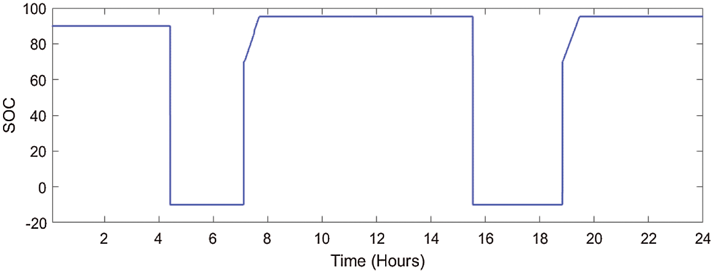
Figure 35: State of charge of batteries for Profile #2 when people going to work with a possibility to charge their car at work but with a longer ride (Total number of cars: 25) for 24 h period
The SOC of batteries for Profile #3 when people go to work without being able to charge their cars at work (Total number of cars: 10) over a 24 h period is depicted in Fig. 36. It is observed that the SOC of the batteries decreases between 5:30 and 18 h while going from home to the workplace in the morning hours, staying at the workplace and returning back to home in the evening hours. Similarly, the SOC also decreases when people return home from the workplace in the evening hours between 15:30 and 19 h. SOC increases during the period of the workplace when batteries are charged at the workplace and becomes high above 90. Since batteries are not charged at work, the SOC is retained at low values for this period. Since the batteries are not charged at work, they are charged in the night hours at home, and for this period, SOC is high.
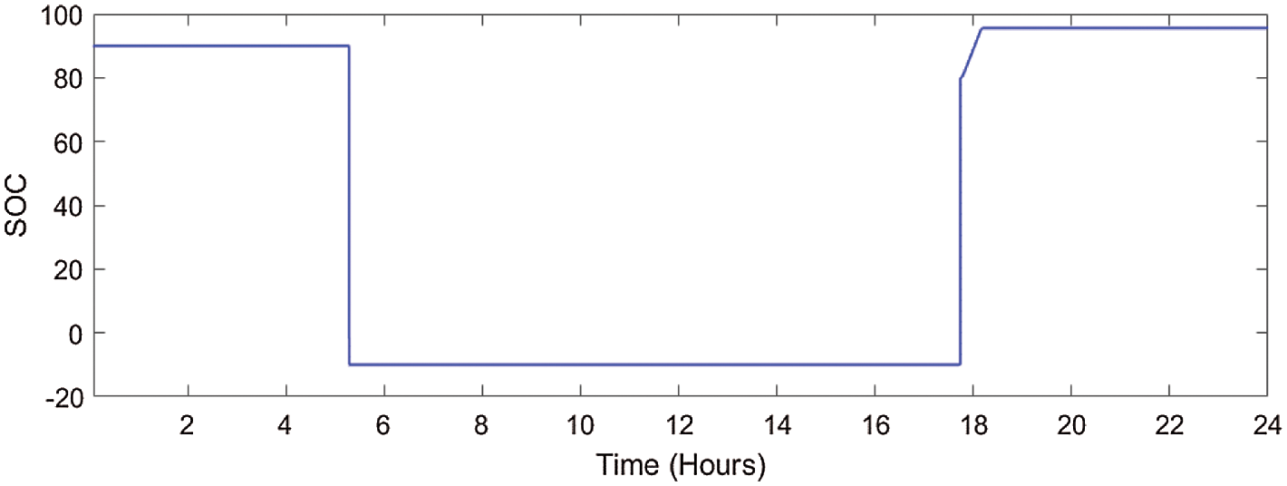
Figure 36: State of charge of batteries for Profile #3 when people going to work with no possibility to charge their car at work (Total number of cars: 10) for 24 h period
The SOC of batteries for Profile #4 when the people stay at home (Total number of cars: 20) over a period of 24 h is described in Fig. 37. It is observed that the SOC of the batteries remains almost constant for the entire period. However, slight variations are observed when cars are used for local, domestic purposes.
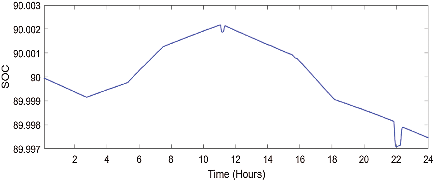
Figure 37: State of charge of batteries for Profile #4 when people staying at home (Total number of cars: 20) for 24 h
The SOC of batteries for Profile #5 when the people are working the night shift and the possibility to charge their cars at home (Total number of cars: 10) over a period of 24 h is described in Fig. 38.
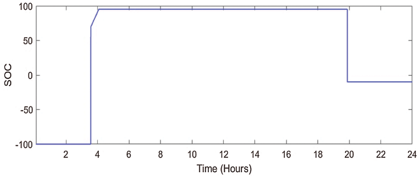
Figure 38: State of charge of batteries for Profile #5 when people working on a night shift (Total number of cars: 10) for 24 h period
It is observed that the SOC of the batteries decreases between 20 h of a day and 4 h of the next day when people are going from home to the workplace in the evening hours, staying at the workplace during the night hours, and returning back to home in the morning hours. SOC increases during the period of daylight hours when people stay at home and there is the possibility to charge cars. Since the batteries are not charged at the workplace, the SOC is retained at low values for the night period.
A vehicle-to-grid system interfaced with a microgrid to meet the load demand and regulate the parameters of the microgrid has been proposed. This design has been achieved for a period of a 24 h cycle. A microgrid has been designed and divided into four components: a diesel generator, PV and wind plants, a V2G system, and the load demand. A microgrid is designed with a suitable size to represent a community of a thousand households during a low-consumption day in spring or fall. A total of 100 EVs have been modelled as base models to realize a 1:10 ratio between cars and households, which indicates a possible scenario in the near future. It is concluded that the proposed design of the microgrid and V2G effectively operates and meets the load demand. All the parameters of the microgrid, such as voltage, current, frequency, and power variations, have been maintained within the permissible limits. V2G has been utilized to regulate variations in the parameters of the system by supplying power from the batteries of the vehicles to the grid. All the results, such as voltage, active power, reactive power, current, wind speed variations, variations in the irradiance, and state of charge of the batteries, have been analyzed, and it is established that the proposed design of the V2G and microgrid effectively regulates all these parameters. The parameters of the microgrid and V2G have been managed by the hit and trial method. It is concluded that the error in the measurement of voltage and frequency for the test grid for different scenarios of V2G vehicles is less than 5%, indicating that the proposed model of V2G and microgrid is not very sensitive to the change in the operating conditions and effectively operates in different operating scenarios. In the future, optimization techniques could be used to improve the performance and efficiency of the energy sources with the aim of effectively managing the loads connected to the grid. The proposed approach will be tested on larger test grids with a large number of nodes in future research.
Funding Statement: The authors received no specific funding for this study.
Conflicts of Interest: The authors declare that they have no conflicts of interest to report regarding the present study.
1. Santis, E. D., Livi, L., Sadeghian, A., Rizzi, A. (2015). Modeling and recognition of smart grid faults by a combined approach of dissimilarity learning and one-class classification. Neurocomputing, 170, 368–383. DOI 10.1016/j.neucom.2015.05.112. [Google Scholar] [CrossRef]
2. Ghazvini, A. M., Olamaei, J. (2019). Optimal sizing of autonomous hybrid PV system with considerations for V2G parking lot as controllable load based on a heuristic optimization algorithm. Solar Energy, 184, 30–39. DOI 10.1016/j.solener.2019.03.087. [Google Scholar] [CrossRef]
3. Noel, L., Rubens, G. Z., Kester, J., Sovacool, B. K. (2018). Beyond emissions and economics: Rethinking the co-benefits of electric vehicles (EVs) and vehicle-to-grid (V2G). Transport Policy, 71, 130–137. DOI 10.1016/j.tranpol.2018.08.004. [Google Scholar] [CrossRef]
4. Sovacool, B. K., Kester, J., Noel, L., Rubens, G. Z. (2019). Are electric vehicles masculinized? Gender, identity, and environmental values in nordic transport practices and vehicle-to grid (V2G) preferences. Transportation Research Part D: Transport and Environment, 72, 187–202. DOI 10.1016/j.trd.2019.04.013. [Google Scholar] [CrossRef]
5. Sovacool, B. K., Kester, J., Noel, L., Rubens, G. Z. (2020). Actors, business models, and innovation activity systems for vehicle-to-grid (V2G) technology: A comprehensive review. Renewable and Sustainable Energy Reviews, 131, 109963. DOI 10.1016/j.rser.2020.109963. [Google Scholar] [CrossRef]
6. Verbong, G. P. J., Beemsterboer, S., Sengers, F. (2013). Smart grids or smart users involving users in developing a low carbon electricity economy. Energy Policy, 52, 117–125. DOI 10.1016/j.enpol.2012.05.003. [Google Scholar] [CrossRef]
7. Yu, M., Hong, S. H. (2016). A real-time demand-response algorithm for smart grids: A stackelberg game approach. IEEE Transactions on Smart Grid, 7(2), 879–888. DOI 10.1109/TSG.2015.2413813. [Google Scholar] [CrossRef]
8. Gungor, V. C., Sahin, D., Kocak, T., Ergut, S., Buccella, C. et al. (2013). A survey on smart grid potential applications and communication requirements. IEEE Transactions on Industrial Informatics, 9(1), 28–42. DOI 10.1109/TII.2012.2218253. [Google Scholar] [CrossRef]
9. Deng, R., Xiao, G., Lu, R., Chen, J. (2015). Fast distributed demand response with spatially and temporally coupled constraints in smart grid. IEEE Transactions on Industrial Informatics, 11(6), 1597–1606. DOI 10.1109/TII.2015.2408455. [Google Scholar] [CrossRef]
10. Le, T. T. M., Retiere, N. (2014). Exploring the scale-invariant structure of smart grids. IEEE Systems Journal, 99, 1–10. DOI 10.1109/JSYST.2014.2359052. [Google Scholar] [CrossRef]
11. Amin, S. M., Wollenberg, B. F. (2005). Toward a smart grid: Power delivery for the 21st century. IEEE Power and Energy Magazine, 3(5), 35–41. DOI 10.1109/MPAE.2005.1507024. [Google Scholar] [CrossRef]
12. Real, A. J. D., Arce, A., Bordons, C. (2014). Combined environmental and economic dispatch of smart grids using distributed model predictive control. International Journal of Electrical Power Energy Systems, 54, 65–76. DOI 10.1016/j.ijepes.2013.06.035. [Google Scholar] [CrossRef]
13. Hu, Q., Li, F., Chen, C. F. (2015). A smart home test bed for undergraduate education to bridge the curriculum gap from traditional power systems to modernized smart grids. IEEE Transactions on Education, 58(1), 32–38. DOI 10.1109/TE.2014.2321529.0. [Google Scholar] [CrossRef]
14. Chanda, S., De, A. (2014). A Multi-objective solution algorithm for optimum utilization of smart grid infrastructure towards social welfare. International Journal of Electrical Power Energy Systems, 58, 307–318. DOI 10.1016/j.ijepes.2014.01.029. [Google Scholar] [CrossRef]
15. Goulden, M., Bedwell, B., Rennick-Egglestone, S., Rodden, T., Spence, A. (2014). Smart grids, smart users, the role of the user in demand side management. Energy Research Social Science, 2, 21–29. DOI 10.1016/j.erss.2014.04.008. [Google Scholar] [CrossRef]
16. Evora, J., Hernandez, J. J., Hernandez, M. (2015). A MOPSO method for direct load control in smart grid. Expert Systems with Applications, 42(21), 7456–7465. DOI 10.1016/j.eswa.2015.05.056. [Google Scholar] [CrossRef]
17. Karimi, B., Namboodiri, V., Jadliwala, M. (2015). Scalable meter data collection in smart grids through message concatenation. IEEE Transactions on Smart Grid, 6(4), 1697–1706. DOI 10.1109/TSG.2015.2426020. [Google Scholar] [CrossRef]
18. Liang, J., Venayaga moorthy, G. K., Harley, R. G. (2012). Wide-area measurement based dynamic stochastic optimal power flow control for smart grids with high variability and uncertainty. IEEE Transactions on Smart Grid, 3(1), 59–69. DOI 10.1109/TSG.2011.2174068. [Google Scholar] [CrossRef]
19. Milioudis, A. N., Andreou, G. T., Labridis, D. P. (2012). Enhanced protection scheme for smart grids using power line communications techniques. IEEE Transactions on Smart Grid, 3(4), 1631–1640. DOI 10.1109/TSG.2012.2208987. [Google Scholar] [CrossRef]
20. Claessen, F. N., Claessens, B., Hommelberg, M. P. F., Molderink, A., Bakker, V. et al. (2014). Comparative analysis of tertiary control systems for smart grids using the flex street model. Renewable Energy, 69, 260–270. DOI 10.1016/j.renene.2014.03.037. [Google Scholar] [CrossRef]
21. Cecati, C., Mokryani, G., Piccolo, A., Siano, P. (2010). An overview on the smart grid concept. 36th Annual Conference on IEEE Industrial Electronics Society, pp. 3322–3327. Glendale, AZ, USA. DOI 10.1109/IECON.2010.5675310. [Google Scholar] [CrossRef]
22. Tenti, P., Paredes, H. K. M., Mattavelli, P. (2011). Conservative power theory, a framework to approach control and accountability issues in smart microgrids. IEEE Transactions on Power Electronics, 26(3), 664–673. DOI 10.1109/TPEL.2010.2093153. [Google Scholar] [CrossRef]
23. Gamage, T. T., Roth, T. P., Mc Millin, B. M., Crow, M. L. (2013). Mitigating event confidentiality violations in smart grids: An information flow security based approach. IEEE Transactions on Smart Grid, 4(3), 1227–1234. DOI 10.1109/TSG.2013.2243924. [Google Scholar] [CrossRef]
24. Tuballa, M. L., Abundo, M. L. (2016). A review of the development of smart grid technologies. Renewable and Sustainable Energy Reviews, 59, 710–725. DOI 10.1016/j.rser.2016.01.011. [Google Scholar] [CrossRef]
25. Al-Anbagi, I., Erol-Kantarci, M., Mouftah, H. T. (2014). Priority- and delay aware medium access for wireless sensor networks in the smart grid. IEEE Systems Journal, 8(2), 608–618. DOI 10.1109/JSYST.2013.2260939. [Google Scholar] [CrossRef]
26. Huang, J., Wang, H., Qian, Y., Wang, C. (2013). Priority based traffic scheduling and utility optimization for cognitive radio communication infrastructure-based smart grid. IEEE Transactions on Smart Grid, 4(1), 78–86. DOI 10.1109/TSG.2012.2227282. [Google Scholar] [CrossRef]
27. Li, Z., Liang, Q. (2015). Capacity optimization in heterogeneous home area networks with application to smart grid. IEEE Transactions on Vehicular Technology, 99, 1–11. DOI 10.1109/TVT.2015.2402219. [Google Scholar] [CrossRef]
28. Ancillotti, E., Bruno, R., Conti, M. (2013). The role of the RPL routing protocol for smart grid communications. IEEE Communications Magazine, 51(1), 75–83. DOI 10.1109/MCOM.2013.6400442. [Google Scholar] [CrossRef]
29. Pang, C., Dutta, P., Kezunovic, M. (2012). BEVs/PHEVs as dispersed energy storage for V2B uses in the smart grid. IEEE Transactions on Smart Grid, 3(1), 473–482. DOI 10.1109/TSG.2011.2172228. [Google Scholar] [CrossRef]
30. Deng, R., Yang, Z., Chen, J., Chow, M. Y. (2014). Load scheduling with price uncertainty and temporally-coupled constraints in smart grids. IEEE Transactions on Power Systems, 29(6), 2823–2834. DOI 10.1109/TPWRS.2014.2311127. [Google Scholar] [CrossRef]
31. Liu, Y., Yuen, C., Yu, R., Zhang, Y., Xie, S. (2015). Queuing-based energy consumption management for heterogeneous residential demands in smart grid. IEEE Transactions on Smart Grid, 7(3), 1650–1659. DOI 10.1109/TSG.2015.2432571. [Google Scholar] [CrossRef]
32. Kumano, T., Horita, M., Shinada, M., Li, X. (2019). A study onV2G based frequency control in power grid with renewable energy. IFAC Papers on Line, 52(4), 99–104. DOI 10.1016/j.ifacol.2019.08.162. [Google Scholar] [CrossRef]
33. Krueger, H., Cruden, A. (2020). Integration of electric vehicle user charging preferences into vehicle-to-grid aggregator controls. In: Energy reports, vol. 6, pp. 86–95. 4th Annual CDT Conference in Energy Storage and Its Applications, University of Southampton, UK. [Google Scholar]
34. Meesenburg, W., Thingvad, A., Elmegaard, B., Marinelli, M. (2020). Combined provision of primary frequency regulation from vehicle-to-grid (V2G) capable electric vehicles and community-scale heat pump. Sustainable Energy, Grids and Networks, 23, 100382. DOI 10.1016/j.segan.2020.100382. [Google Scholar] [CrossRef]
35. Al-Anbagi, I., Mouftah, H. T. (2016). WAVE 4 V2G: Wireless access in vehicular environments for vehicle-to-grid applications. Vehicular Communications, 3, 31–42. DOI 10.1016/j.vehcom.2015.12.002. [Google Scholar] [CrossRef]
36. Bamisile, O., Obiora, S., Huang, Q., Okonkwo, E. C., Olagoke, O. et al. (2020). Towards a sustainable and cleaner environment in China: Dynamic analysis of vehicle-to-grid, batteries and hydro storage for optimal RE integration. Sustainable Energy Technologies and Assessments, 42, 100872. DOI 10.1016/j.seta.2020.100872. [Google Scholar] [CrossRef]
37. Roman, L. F. A., Gondim, P. R. L., Lloret, J. (2019). Pairing-based authentication protocol for V2G networks in smart grid. Ad Hoc Networks, 90, 101745. DOI 10.1016/j.adhoc.2018.08.015. [Google Scholar] [CrossRef]
38. Kestera, J., Rubens, G. Z., Sovacoolb, B. K., Noel, L. (2019). Public perceptions of electric vehicles and vehicle-to-grid (V2GInsights from a nordic focus group study. Transportation Research, 74, 277–293. DOI 10.1016/j.trd.2019.08.006. [Google Scholar] [CrossRef]
39. Egbue, O., Uko, C. (2020). Multi-agent approach to modeling and simulation of microgrid operation with vehicle-to-grid system. The Electricity Journal, 33, 106714. DOI 10.1016/j.tej.2020.106714. [Google Scholar] [CrossRef]
40. Biresselioglu, M. E., Kaplan, M. D., Yilmaz, B. K. (2018). Electric mobility in Europe: A comprehensive review of motivators and barriers in decision making processes. Transportation Research Part A: Policy and Practice, 109, 1–13. DOI 10.1016/j.tra.2018.01.017. [Google Scholar] [CrossRef]
41. Yu, R., Zhong, W., Xie, S., Yuen, C., Gjessing, S. et al. (2016). Balancing power demand through EV mobility in vehicle-to-grid mobile energy networks. IEEE Transactions on Industrial Informatics, 12, 79–90. DOI 10.1109/TII.2015.2494884. [Google Scholar] [CrossRef]
42. Bilgin, B., Magne, P., Malysz, P., Yang, Y., Pantelic, V. et al. (2015). Making the case for electrified transportation. IEEE Transactions on Transportation Electrification, 1, 4–17. DOI 10.1109/TTE.2015.2437338. [Google Scholar] [CrossRef]
43. Dallinger, D., Gerda, S., Wietschel, M. (2013). Integration of intermittent renewable power supply using grid-connected vehicles: A 2030 case study for california and Germany. Applied Energy, 104, 666–682. DOI 10.1016/j.apenergy.2012.10.065. [Google Scholar] [CrossRef]
44. Schuller, A., Flath, C. M., Gottwalt, S. (2015). Quantifying load flexibility of electric vehicles for renewable energy integration. Applied Energy, 151, 335–344. DOI 10.1016/j.apenergy.2015.04.004. [Google Scholar] [CrossRef]
45. Shyam, B., Kanakasabapathy, P. (2018). Large scale electrical energy storage systems in India-current status and future prospects. Journal of Energy Storage, 18, 112–120. DOI 10.1016/j.est.2018.04.018. [Google Scholar] [CrossRef]
46. Aldik, A., Al-Awami, A. T., Sortomme, E., Muqbel, A. M., Shahidehpour, M. (2018). A planning model for electric vehicle aggregators providing ancillary services. IEEE Access, 6, 70685–70697. DOI 10.1109/Access.6287639. [Google Scholar] [CrossRef]
47. Mohamed, M. A., Abdullah, H. M., El-Meligy, M. A., Sharaf, M., Soliman, A. T. et al. (2021). A novel fuzzy cloud stochastic framework for energy management of renewable microgrids based on maximum deployment of electric vehicles. Electrical Power and Energy Systems, 129, 106845. DOI 10.1016/j.ijepes.2021.106845. [Google Scholar] [CrossRef]
48. Wang, P., Wang, D., Zhu, C., Yang, Y., Abdullah, H. M. et al. (2020). Stochastic management of hybrid AC/DC microgrids considering electric vehicles charging demands. Energy Reports, 6, 1338–1352. DOI 10.1016/j.egyr.2020.05.019. [Google Scholar] [CrossRef]
49. Gong, X., Dong, F., Mohamed, M. A., Abdalla, O. M., Ali, Z. M. (2020). A secured energy management architecture for smart hybrid microgrids considering PEM-fuel cell and electric vehicles. IEEE Access, 8, 47807–47823. DOI 10.1109/Access.6287639. [Google Scholar] [CrossRef]
50. Avatefipour, O., Al-Sumaiti, A. S., El-Sherbeeny, A. M., Awwad, E. M., Elmeligy, M. A. et al. (2019). An intelligent secured framework for cyberattack detection in electric vehicles’ CAN bus using machine learning. IEEE Access, 7, 127580–127592. DOI 10.1109/Access.6287639. [Google Scholar] [CrossRef]
51. Lan, T., Jermsittiparsert, K., Alrashood, S. T., Rezaei, M., Al-Ghussain, L. et al. (2021). An advanced machine learning based energy management of renewable microgrids considering hybrid electric vehicles’ charging demand. Energies, 14, 569. DOI 10.3390/en14030569. [Google Scholar] [CrossRef]
52. Neofytou, N., Blazakis, K., Katsigiannis, Y., Stavrakakis, G. (2019). Modeling vehicles to grid as a source of distributed frequency regulation in isolated grids with significant RES penetration. Energies, 12, 720. DOI 10.3390/en12040720. [Google Scholar] [CrossRef]
53. Honarmand, M., Zakariazadeh, A., Jadid, S. (2014). Optimal scheduling of electric vehicles in an intelligent parking lot considering vehicle-to-grid concept and battery condition. Energy, 65, 572–579. DOI 10.1016/j.energy.2013.11.045. [Google Scholar] [CrossRef]
 | This work is licensed under a Creative Commons Attribution 4.0 International License, which permits unrestricted use, distribution, and reproduction in any medium, provided the original work is properly cited. |