| Energy Engineering |
DOI: 10.32604/ee.2022.020283
ARTICLE
Short-Term Prediction of Photovoltaic Power Based on Fusion Device Feature-Transfer
1College of Electrical Engineering, Liaoning University of Technology, Jinzhou, 121001, China
2School of Electrical Engineering, Shandong University, Jinan, 250012, China
*Corresponding Author: Zhongyao Du. Email: druid_y@live.com
Received: 15 November 2021; Accepted: 18 February 2022
Abstract: To attain the goal of carbon peaking and carbon neutralization, the inevitable choice is the open sharing of power data and connection to the grid of high-permeability renewable energy. However, this approach is hindered by the lack of training data for predicting new grid-connected PV power stations. To overcome this problem, this work uses open and shared power data as input for a short-term PV-power-prediction model based on feature transfer learning to facilitate the generalization of the PV-power-prediction model to multiple PV-power stations. The proposed model integrates a structure model, heat-dissipation conditions, and the loss coefficients of PV modules. Clear-Sky entropy, characterizes seasonal and weather data features, describes the main meteorological characteristics at the PV power station. Taking gate recurrent unit neural networks as the framework, the open and shared PV-power data as the source-domain training label, and a small quantity of power data from a new grid-connected PV power station as the target-domain training label, the neural network hidden layer is shared between the target domain and the source domain. The fully connected layer is established in the target domain, and the regularization constraint is introduced to fine-tune and suppress the overfitting in feature transfer. The prediction of PV power is completed by using the actual power data of PV power stations. The average measures of the normalized root mean square error (NRMSE), the normalized mean absolute percentage error (NMAPE), and the normalized maximum absolute percentage error (NLAE) for the model decrease by 15%, 12%, and 35%, respectively, which reflects a much greater adaptability than is possible with other methods. These results show that the proposed method is highly generalizable to different types of PV devices and operating environments that offer insufficient training data.
Keywords: Solar power generation; transfer learning; PV module; UMAP; GRU; overfitting
Nomenclature
| DS | Source domain dataset |
| DT | Target domain dataset |
| IE | Effective irradiance (W/m2) |
| ID | Direct irradiance (W/m2) |
| IDIF | Diffuse irradiance (W/m2) |
| IG | Global irradiance (W/m2) |
| θ | Solar declination angle on PV array (°) |
| β | PV array inclination (°) |
| γ | PV array azimuth (°) |
| μ | Ground reflection coefficient |
| α | Solar altitude angle (°) |
| γs | Solar altitude azimuth (°) |
| ε | Solar altitude declination angle (°) |
| ω | Hour angle (°) |
| φ | Local latitude (°) |
| t | Time (minutes) |
| Tm | Module temperature (°C) |
| Tamb | Ambient temperature (°C) |
| v | Actual wind speed (m/s) |
| vw | Wind speed in weather dataset (m/s) |
| h | Device height (m) |
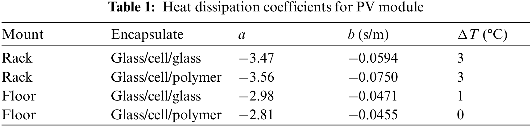
| a, b | heat dissipation coefficient |
| LP | System losses (%) |
| LLID | Light-induced degradation losses (%) |
| LN | Nominal losses (%) |
| LS | Shadow Losses (%) |
| IC | Clear-Sky irradiance (W/m2) |
| d | Euclidean distance |
| M | Fuzzy function |
| σ | Standard deviation |
| EC | Clear-Sky entropy |
| SC | Seasonal characteristic coefficient |
| SG | Seasonal grade |
| Idmax | Daily maximum effective irradiance (W/m2) |
| Iimax | Maximum effective irradiance of ideal value in current season (W/m2) |
| Gij | Joint probability distribution of any two origin-data points |
| Qij | Joint probability distribution of any two features |
| k, p, q | UMAP hyperparameter |
| CE | Cross entropy |
| U | Weather feature dataset |
| Zt | Update gate |
| Rt | Reset gate |
| xt | Input state |
| ht | Hidden state |
| W | Weight matrix |
| δ | Neural network parameter |
| l | Dataset of label |
| F | Dataset of feature |
| λ | L2 regularization penalty coefficient |
To attain the goal of carbon peaking and carbon neutrality, estimates indicate that the fraction of power generation from renewable energy in China must increase from the current 8% to over 60% by 2060 [1]. Unfortunately, power generation from renewable energy is intermittent, with random and volatile fluctuations in power output [2]. In particular, modern photovoltaic (PV) power stations lack power data labels, and their power output is difficult to predict with accuracy. Connecting such power stations to the large-scale power grid makes it challenging to maintain the stable operation of the power grid [3]. Accurate short-term forecasting of PV power generation is thus urgently needed for the day-ahead forecasting of PV power input into the power grid [4,5] and would significantly improve PV penetration into the power grid, thereby making a major step toward the goal of net-zero carbon dioxide emissions.
Short-term prediction of PV power generation essentially combines a physical model with a statistical model. Given the limited knowledge of the mechanism and the lack of corrective feedback, the physical model is rarely used alone [6]. Statistical models include the time series analysis method [7] and the machine learning method [8]. The literature widely discusses the machine learning method [9], which is highly generalizable for nonlinear mapping. For example, Chu et al. [10] developed the reforecasting method, which is based on artificial neural network optimization schemes and improves the performance of physical deterministic models based on cloud-tracking techniques. Nie et al. [11] proposed a framework that classifies input images of the sky into various sky conditions and then sends the classified images to specific convolutional neural network models to predict PV power output. These artificial neural network models can approximate the nonlinear relationship between the input features and the prediction target.
Moreover, the time series analysis and physical models in question are based on proven mathematical theories that can rapidly map features, which promotes the emergence of hybrid prediction models that offer multiple advantages [12]. Wang et al. [13] used time correlation modification in an integrated long-short-term memory (LSTM) recurrent neural network algorithm to calculate solar irradiance and PV power generation, which provided more accurate predictions than traditional machine learning models. In other work, Gao et al. [14] divided the daily weather conditions into ideal and non-ideal weather and developed a prediction model based on a LSTM neural network to efficiently map dynamic characteristics of both ideal and non-ideal weather. Adar et al. [15] used principal component analysis (PCA) to extract two principal components from 11 input variables for three technical types of PV modules to conveniently calculate the performance of each PV module.
Despite these advances, the application of machine learning algorithms in the power-generation industry remains challenging due to the lack of training data, especially for new PV power plants. To address this issue, Lee et al. [16] applied an online learning algorithm to gradually improve the adaptability of an algorithm for predicting PV power. Compared with the fixed model, the online algorithm predicts PV power with significantly greater accuracy. In addition, Wang et al. [17] studied the use of the generative adversarial network to expand a extreme weather training dataset.
Another solution to this problem originates from the open- and shared-power dataset, which is a new production factor [18]. Using this dataset, we develop in the present work a short-term PV-power-prediction model based on fusion device feature-transfer (FFT). Specifically, Section 2 proposes applying a feature-fusion method to PV modules and adopts as parameters for the PV module its effective irradiance, temperature (considering heat dissipation), and system losses. The physical characteristics of the different technical types of PV modules are integrated. We then propose a local meteorological model for predicting PV power. The model extract the Clear-Sky entropy, seasonal and weather features to characterize the main meteorological (Section 3). Section 4 introduces a transfer learning (TL) neural network based on a gated recurrent unit (GRU) and a fully connected (FC) layer with fine-tuning and regularization constraints in feature-transfer to localize the prediction model. Section 5 evaluates the ability of the uniform manifold approximation and projection dimension reduction (UMAP) algorithm to extract a weather dataset given the global structure, redundancy, projection time, and feature-set fitting efficiency. Finally, we compare the PV-power predictions and errors produced by the local model, no-TL model, TL-PV model, and FFT-PV model and analyze the operation of the proposed model when localized to a specific environment.
2 Characteristics of Photovoltaic Modules
The TL training set can be divided into source domain DS and target domain DT, where DS is the historical power data of PV plants that have long operated while connected to the grid, and DT is the power data from new PV plants. In TL, the effective irradiance, PV module temperature, and PV system loss are used to model the characteristics of PV modules so that the different types of PV modules can be mapped to a single feature space, thereby reducing differences between distributions to the different domains.
To account for PV devices with different tracker systems, the effective solar irradiance on the PV array must be accurately modeled [19]. This section calculates the irradiance for a fixed PV array or a PV array with a single-axis tracker or a dual-axis tracker. To begin, the effective irradiance IE of a PV array is calculated by using
where ID is the direct irradiance (W/m2), IDIF is the diffuse irradiance (W/m2), IG is the global irradiance (W/m2), θ is the solar declination angle with respect to the PV array (degrees), β is the inclination of the PV array (degrees), and μ is the ground reflection coefficient. When the system is fixed or has a single-axis tracker, β is the installed angle.
The solar declination angle θ is
where α is the solar altitude angle (degrees), γ is the PV array azimuth (degrees), and γs is the solar azimuth (degrees). When the PV array is fixed, γ is the installed value.
The solar azimuth γs and solar altitude angle α are given by
where ε is the solar declination angle (degrees), ω is the hour angle (degrees), φ is the local latitude (degrees), n is the number of days since January 01 [20], and t is the time of day in 24-hour format.
The temperature of the PV module strongly affects the power generation, so accurately calculating the temperature is vital to improve the PV-power-prediction accuracy [21]. The heat dissipation of the PV module is affected by its mounting [22] and encapsulating materials [23]. This section quantifies how the installation orientation of PV modules and the module materials affect the heat dissipation. The temperature of the PV module is given by
where Tamb is the ambient air temperature (°C), a and b are the heat dissipation coefficients (given in Table 1 [24]), v is the actual wind speed (m/s), vw is the wind speed from the weather dataset (m/s), and h is the height of the PV module (m).
The PV power is affected by its local geographical environment, the degradation of facilities, and other factors [25]. The system losses LP are expressed in the form of a percentage:
where Li is the set of LLID, LN, and LS [LLID is the light-induced degradation (LID) losses (%), LN is the nominal loss (%), and LS is the shadow loss (%)]. Initially LLID = 1.5% for a PV array, and it increases by 0.5% per year [26]. The default shading loss for an “unshaded” PV module is 3% [27], which increases if the shadow area in the all-sky imager is calculated.
3 Main Meteorological Characteristics
To account for the influence of meteorological conditions, the solar irradiance is calculated based on the effective irradiance IE and the ideal irradiance IC, where IC is the maximum irradiance not affected by atmospheric conditions (i.e., the Clear-Sky irradiance [28]). We use fuzzy entropy [29] to calculate the self-similarity of the difference x(t) between IC and IE, and the Clear-Sky entropy EC serves to quantify the uncertainty of the weather conditions. The calculation is done in the following steps:
(1) Reconstruct the phase space of the time series x(t) and set the dimension to m:
(2) The distance dij separates the sequence x(i) from the sequence x(j):
(3) Calculate the similarity Mijm between sequences by using the fuzzy function:
where σ is the standard deviation of the time series x(t).
(4) Calculate the similarity of each j and take the average, then repeat Steps 1–3 to calculate the average of each i, which is given as
(5) The Clear-Sky entropy EC of this time series is
During effective power generation, the short-term power prediction calculates the Clear-Sky entropy EC in intervals of four hours.
The ideal solar irradiance varies seasonally with a strong time correlation. However, the effective irradiance is random, which is not conducive to extracting time-series features. Fig. 1 shows the annual irradiance.
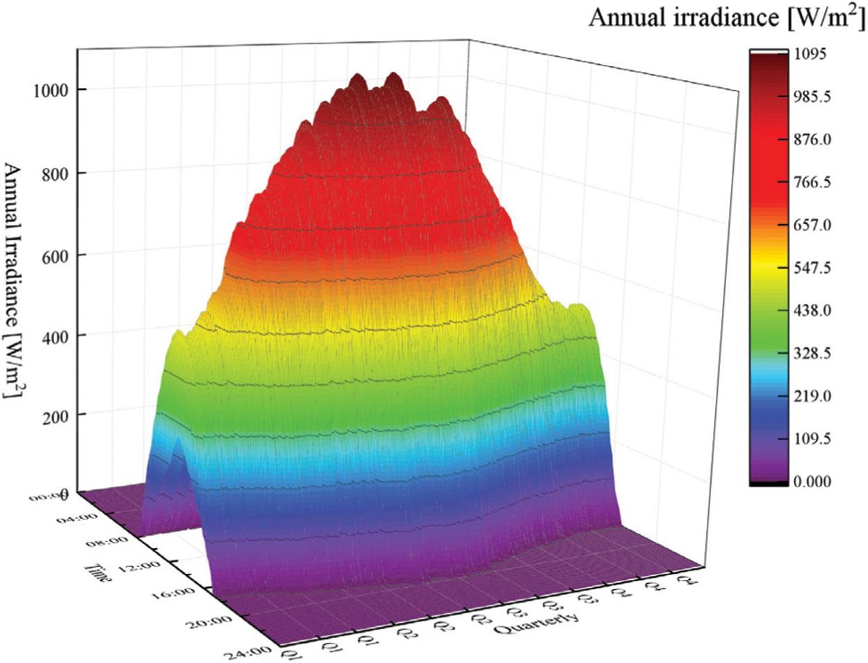
Figure 1: Annual irradiance as a function of time of day and month of year
To improve the efficiency with which the irradiance time series characteristics are recognized, we divide the irradiance into four levels and construct the seasonal characteristic coefficient SC to quantify the irradiance time series, as follows:
where SG is the seasonal grade (i.e., the average irradiance of each of the four seasons from small to large are denoted grades 1 to 4, respectively), Idmax/Iimax is the uncertainty coefficient (the closer it approaches to unity, the closer the irradiance approaches that of the next season), Idmax is the maximum effective daily irradiance (W/m2), and Iimax is the maximum ideal irradiance in the current season (W/m2).
3.3 Weather Feature Based on Uniform Manifold Approximation
The weather dataset is characterized by numerous features, which ensure a large amount of data and little distinction between features. The feature extraction based on t-distributed stochastic neighbor embedding (t-SNE) affects how the relationship between the original data and the prediction algorithm are recognized due to the loss of global structure. This section uses the UMAP algorithm [30] to construct as follows the features of the weather dataset:
(1) Consider a dataset
(2) The parameter k controls the number of neighbors in the cluster and satisfies
(3) Using ρi, a locally similar data cluster is formed, and the joint probability distribution Gij of any two origin-data points in the space is symmetrically calculated as
(4) Let the feature set U be the probability map modeled by D in low-dimensional space using 1/(1+py2q) rather than the t distribution in t-SNE. The joint probability distribution Qij of any two features of N is then given as
(5) The cross-entropy CE is the loss function and balances the local structure and the total structure. It is calculated as follows:
(6) The graph Laplace initializes the low-dimensional coordinates and uses a spectral embedding projection to a low-dimensional space. Stochastic gradient descent [31] is used to optimize, to calculate the gradient with a random subset, to improve the iterative minimum cross-entropy speed, and to calculate the optimal feature set U. The cross-entropy of the stochastic gradient descent optimization is
where uij is the distance between characteristic data points.
4 Prediction Model of Photovoltaic Power
4.1 Gated Recurrent Unit Framework for Feature Transfer
Compared with the commonly used LSTM, the GRU framework offers the advantages of simple structure and fast calculations [32]. Nevertheless, the prediction model constructed from a traditional GRU neural network cannot predict the output of new PV power plants with sufficient accuracy. Therefore, this section constructs a GRU neural network based on TL (TL-GRU) with one input layer, one output layer, two hidden layers, and one FC layer. The hidden layer is initialized by using the source domain dataset and is shared with the target domain. Fig. 2 shows the structure.
The information transmission through a GRU cell is described by Eqs. (24)–(27):
Gate control. Let Zt be the update gate of the GRU at time t, and let Rt be the reset gate:
where S is the stimulus function sigmoid, xt and ht−1 are the input at the current moment and the hidden state at the previous moment, respectively, and Wx and Wh are the weighting matrix of the input and loop connections, respectively.
State retention. Let ht be the current hidden state of the GRU at time t, and let ht′ be the hidden state at the previous time:
where ⊙ is the Hadamard product.
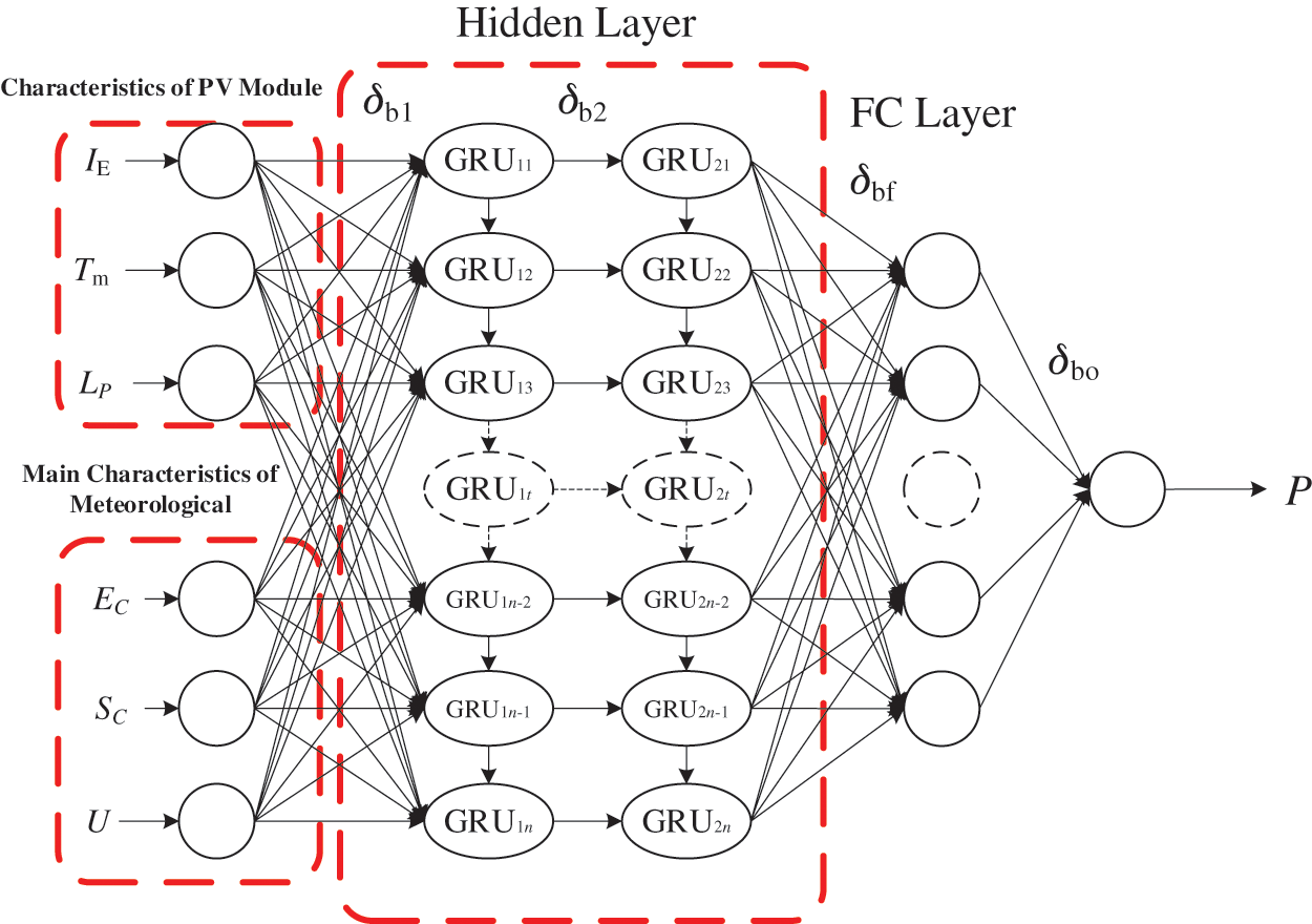
Figure 2: TL-GRU neural network
If the input layer of the neural network is F, then the hidden layers and the output P of the FC layer are
where P is the normalized PV-power prediction (dimensionless), W1, W2, Wf, and Wo are the weighting matrices to transform the input layer to the first hidden layer, the first hidden layer to the second layer, the second hidden layer to the FC layer, and the FC layer to the output layer, respectively, and δb1, δb2, δbf, and δbo are the biases of the two hidden layers, the FC layer, and the output layer, respectively.
4.2 Regularized Transfer Learning
When the prediction model learns the target domain, “catastrophic forgetting” is triggered, which leads to overfitting [33]. The FC layer serves as a “firewall” for TL in this section and is fine-tuned according to the target domain [34].
Let the source domain dataset
where δH is the shared hidden layer parameter, and δSF is the FC layer parameter of the source domain.
Fine-tuning the FC layer over the target domain is problematic because the model becomes excessively complex, and the training process leads to overfitting. We thus introduce a structural penalty on L′ to constrain the model complexity:
where nS is the number of source domain labels, λ is the L2 regularization-penalty coefficient, and W is the regular structural term of the weighting matrix.
Fig. 3 summarizes the steps of the model for short-term prediction of PV power based on the fusion device feature-transfer (FFT-PV) model.
(1) Normalization. To ensure that different features have the same gain as the mapping in the domain, we normalize the data to (0, 1):
(2) Construction of transfer characteristics. We use Eqs. (1)–(9) to calculate the characteristics of the PV modules, then calculate the Clear-Sky entropy EC for 4-hour intervals, and finally construct the main meteorological characteristics together with the Clear-Sky entropy EC, the seasonal characteristic coefficient SC, and the weather feature set U. To summarize, we construct the following transfer characteristics F of the FFT-PV model:
(3) Model pre-training. To establish the TL-GR U framework, we use the source domain
(4) Model localization. We use the source domain
5 Short-Term Prediction of Photovoltaic Power
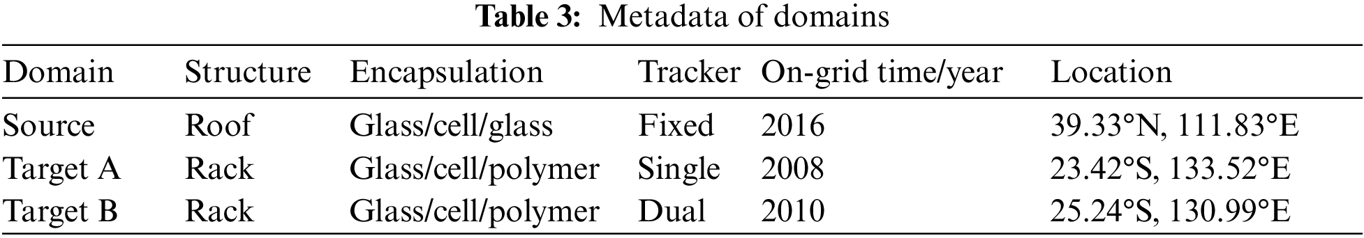
To verify the performance of the FFT-PV model, we use the PV-power data from Pianguan, China [2014/07/26 to 2019/07/26] as the source domain to label lS for 1826 days. The target domain dataset comes from the Desert Knowledge Australia Solar Centre, the power data of [2021/03/09 to 2021/04/09] is target domain A (labeled lTA), and the power data of [2021/02/26 to 2021/03/26] is target domain B (labeled lTB), and both are labeled lT for 30 days. The weather dataset contains ten independent variables: GHI, POA irradiance, DNI, surface pressure, wind direction, wind speed, vertical wind speed, temperature, relative humidity, and rainfall. The time resolution of the power prediction is 15 min, which satisfies the requirements of the grid dispatching agency for short-term renewable-energy forecasting [36].
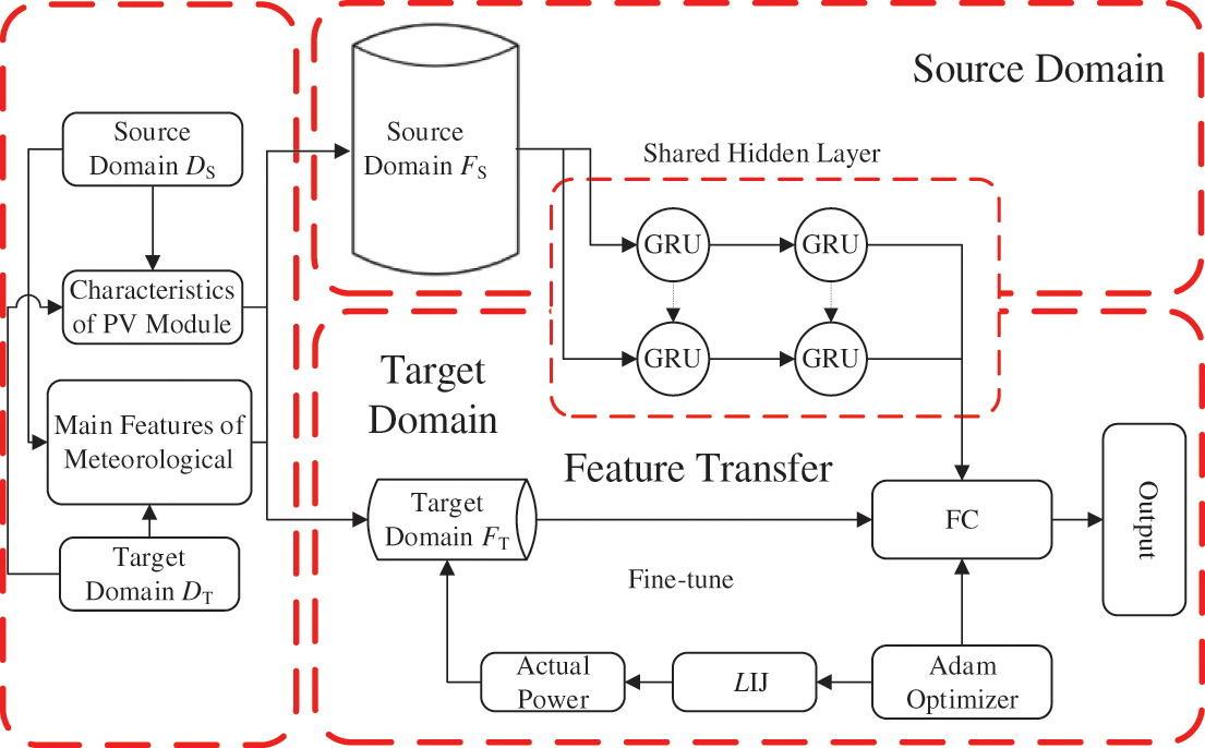
Figure 3: Model for predicting power of PV power plants
5.1 Evaluation of Model Performance
The Spearman correlation coefficient CS represents the correlation between variables, the adjusted correlation coefficient RA2 represents how input affects the model and offsets the contribution to the model of additional variables. The normalized root mean square error (NRMSE) gives the degree of dispersion in the normalized error, the normalized mean absolute percentage error (NMAPE) gives the average normalized percentage error, the normalized maximum absolute percentage error (NLAE) gives the maximum value of the normalized percentage error, and the qualified rate QR is the percent of predicted qualified points with respect to the total number of points in the evaluation period. These quantities are expressed as follows:
where Δi is the difference in grade of a variable (dimensionless), yi, pi, Pmax, and PN are the actual value, predicted value, actual maximum power in the interval, and operating capacity (kW), respectively, and B is the qualified threshold, which is 6.5% in this section.
5.2 Evaluation of Model Feature
The ability of UMAP to extract features from the weather dataset is accurately evaluated and compared with the original dataset D and with the PCA and the t-SNE algorithms.
The global structure is evaluated by the coefficient CS of the distance between the D data points and the distance between the feature set data points (CSD). The average value of the coefficient CS between variables (CSV) evaluates the redundancy between features (see Table 2). The feature set PC exhibits a high redundancy between features, so the global structure is difficult to maintain. CSD = 0.86 for feature set U and CSV = 0.36, which is significantly better than the feature set T. Therefore, UMAP offers the most balance in preserving the global structure.
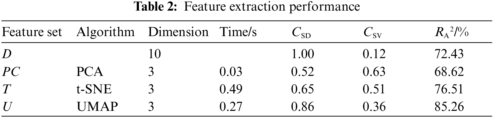
The feature set iteratively trains the neural network, as shown in Fig. 4. The feature sets PC, T, and U can accelerate the iteration speed, but the loss of PC information reduces the accuracy. Comparing the fitting degree of each feature set to the PV power by calculating RA2 shows that feature sets T and U improve the fitting accuracy of features. For U, RA2 = 85.26%, and the calculation time of UMAP decreases by 8.75% with respect to t-SNE.
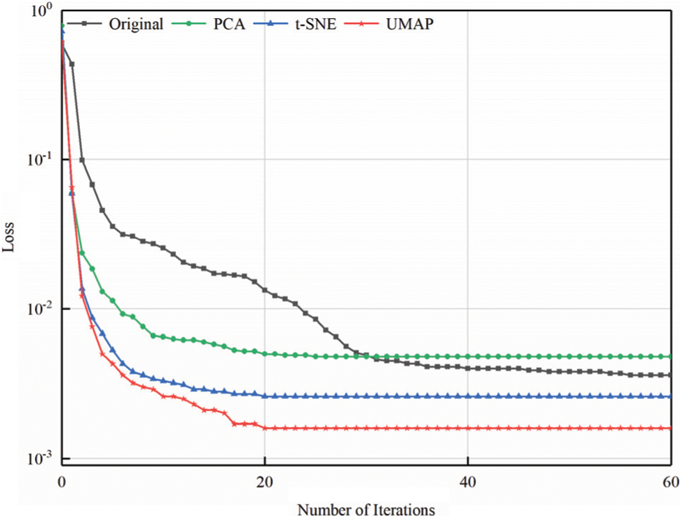
Figure 4: Iteration process for calculating loss
To summarize, the UMAP algorithm rapidly and accurately constructs the weather feature set to replace the original meteorological data.
To test that the FFT-PV model can be easily generalized for use with different PV power stations, Section 5.3.1 evaluates the data mining ability of the prediction model trained by the source domain feature set FS, and Section 5.3.2 transfers learning from the source domain model to target domains A and B and tests the adaptability of the FTL-PV model to different domains. Table 3 lists part of the metadata of each domain.
The source domain model is trained with FS and is based on a GRU neural network. Fig. 5 compares the PV power predicted by the source domain feature set FS with that predicted by the Elman network, the echo state network (ESN), and the LSTM network. Fig. 6 shows QR for the source domain.
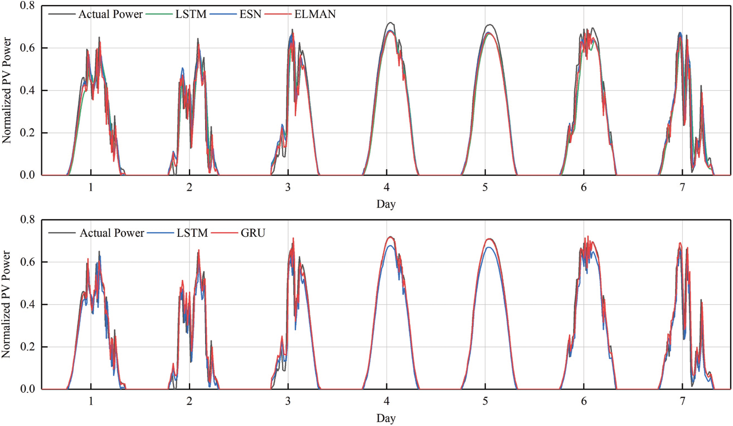
Figure 5: Comparison of source domain predictions
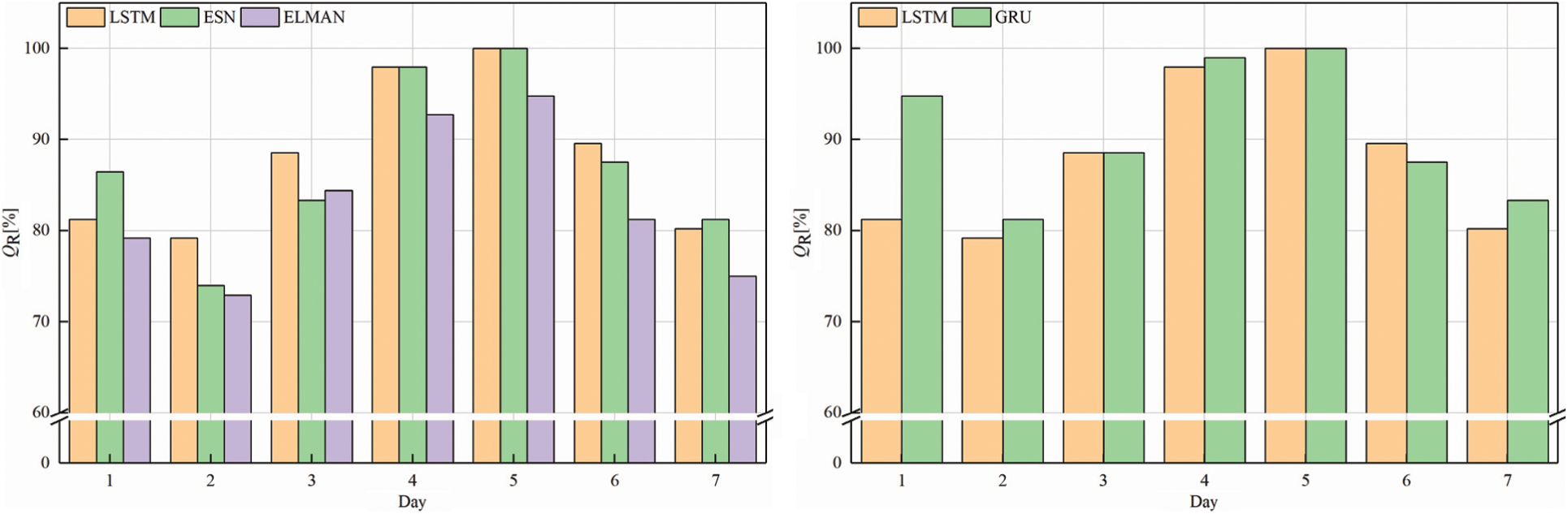
Figure 6: QR of source domain
Fig. 6 shows that the time series-based LSTM and GRU framework produce a greater QR, with the simpler structure of the GRU producing the highest QR. Table 4 lists the prediction indicators of the source domain.
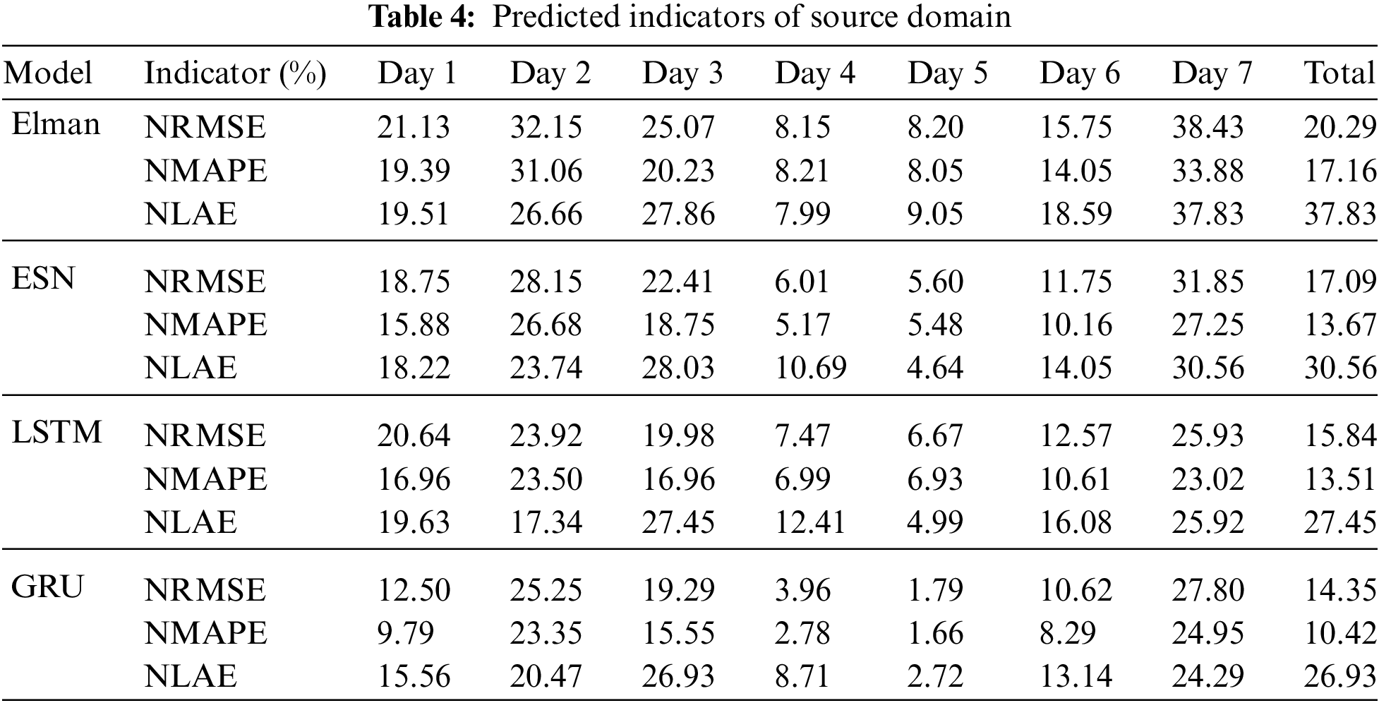
Overall, the indicators of the GRU framework in the source domain are significantly better than those of the other frameworks. On average, the indicators of the GRU framework are reduced by 3% for NRMSE, 4% for NMAPE, and 5% for NLAE. Therefore, the GRU network based on time series produces the most accurate PV-power forecasts of all frameworks studies herein.
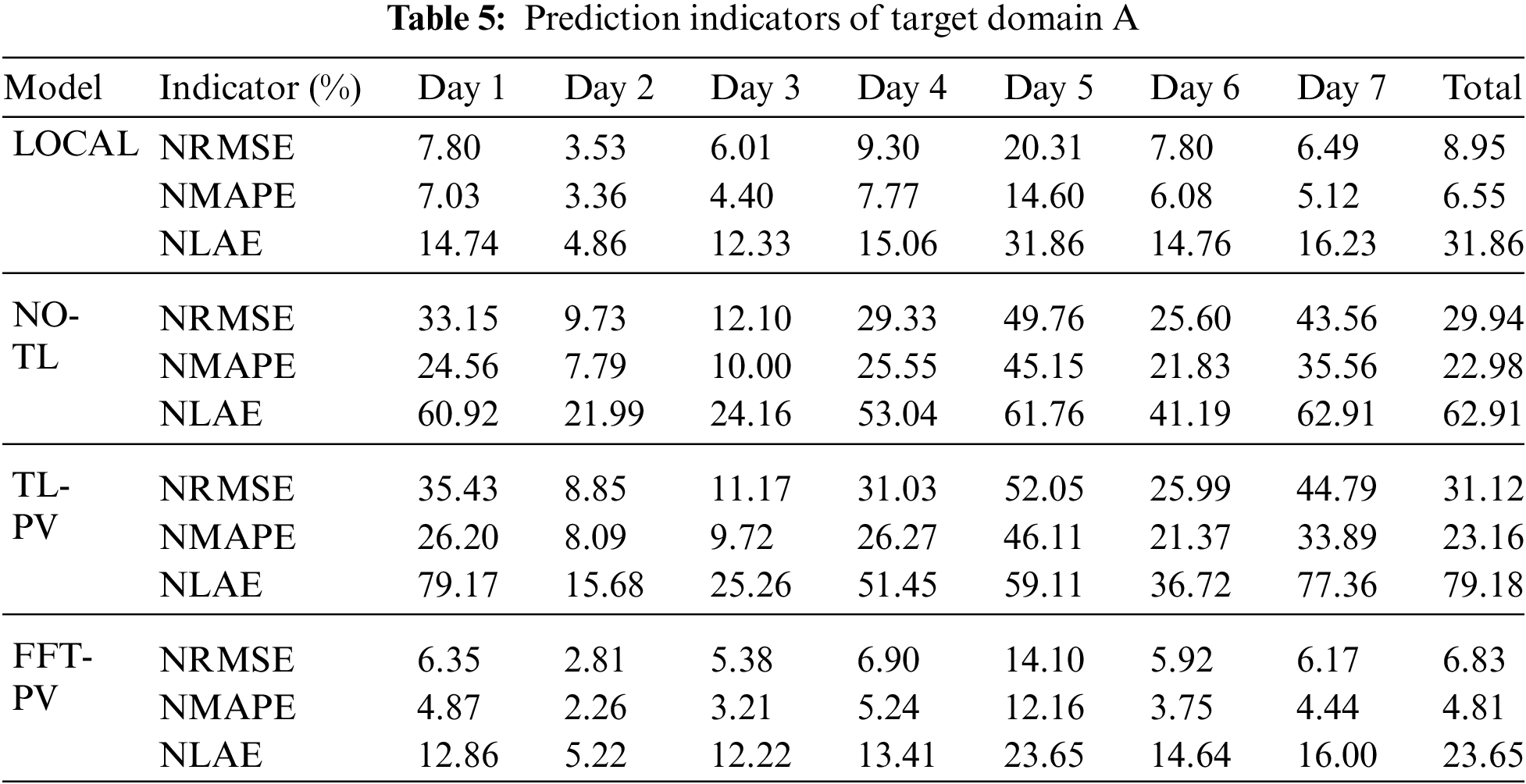
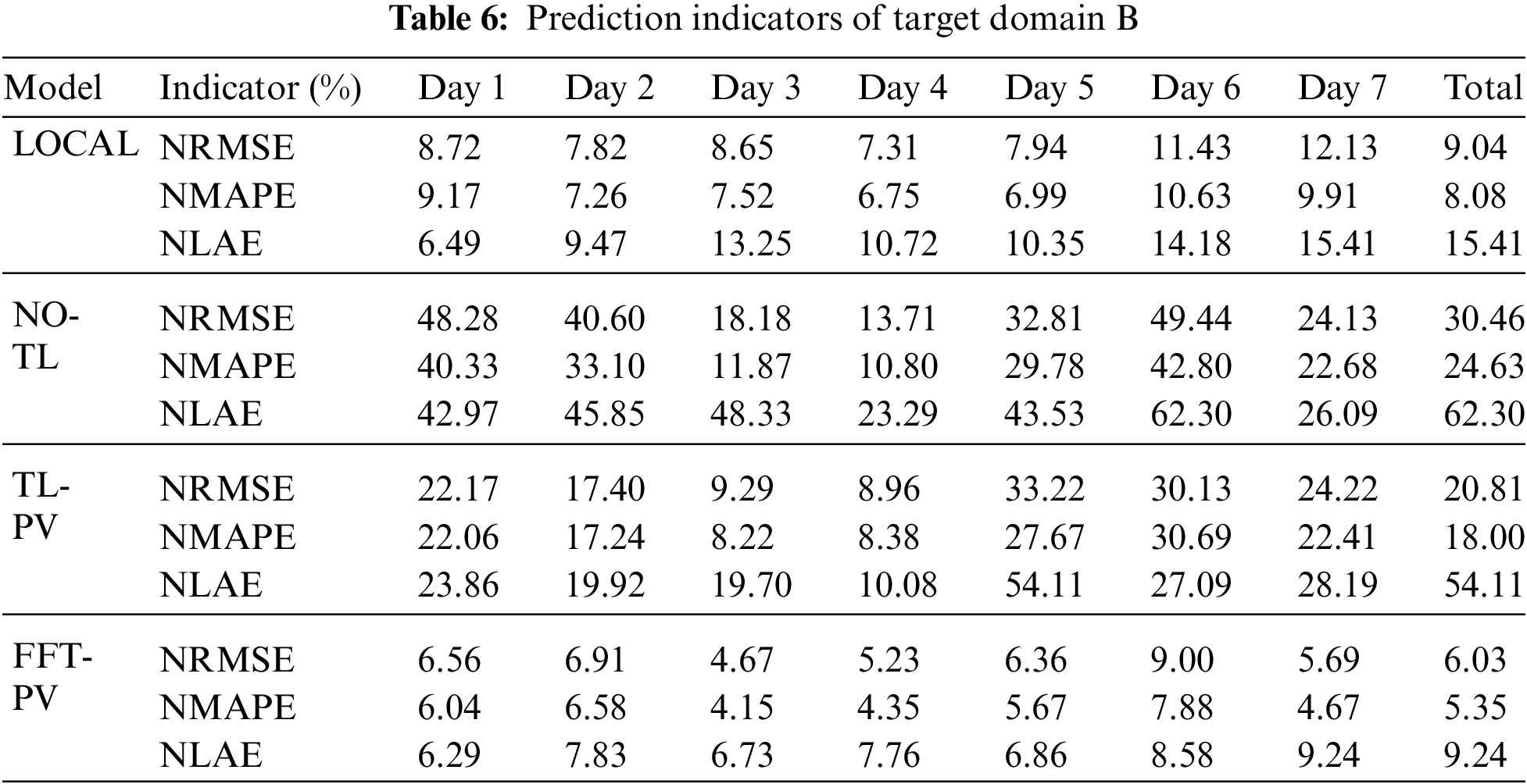
To verify the generalizability of feature transfer, TL is applied to the target domains A and B, and the FFT-PV model is compared with the no-TL model, the prediction model based on the local dataset (LOCAL), and the TL model without constructing the characteristics of the PV module (TL-PV) in Figs. 7–10 and Tables 5, 6 present the results for target domain A (B).
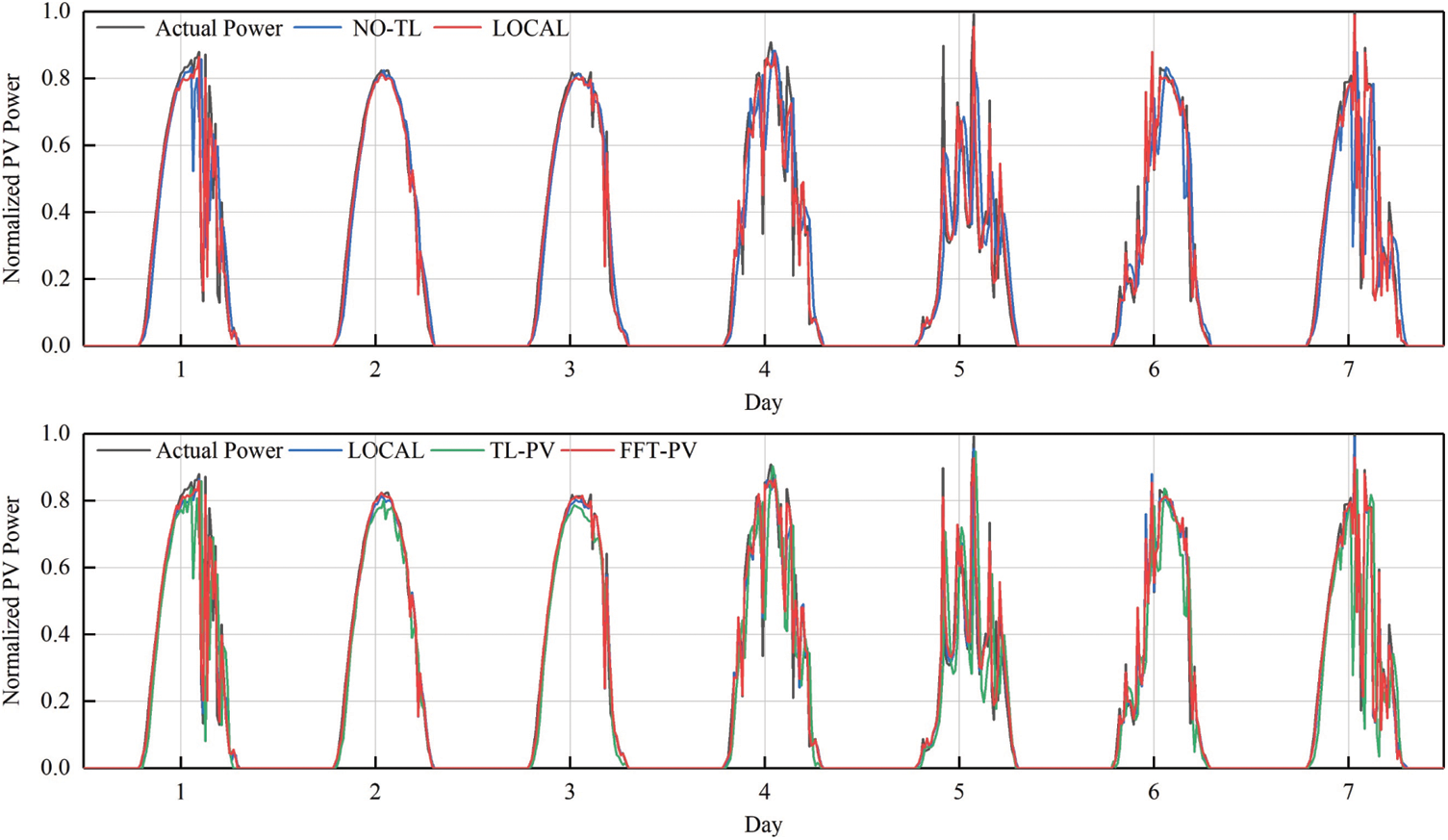
Figure 7: Comparison of PV-power predictions of the various models in target domain A
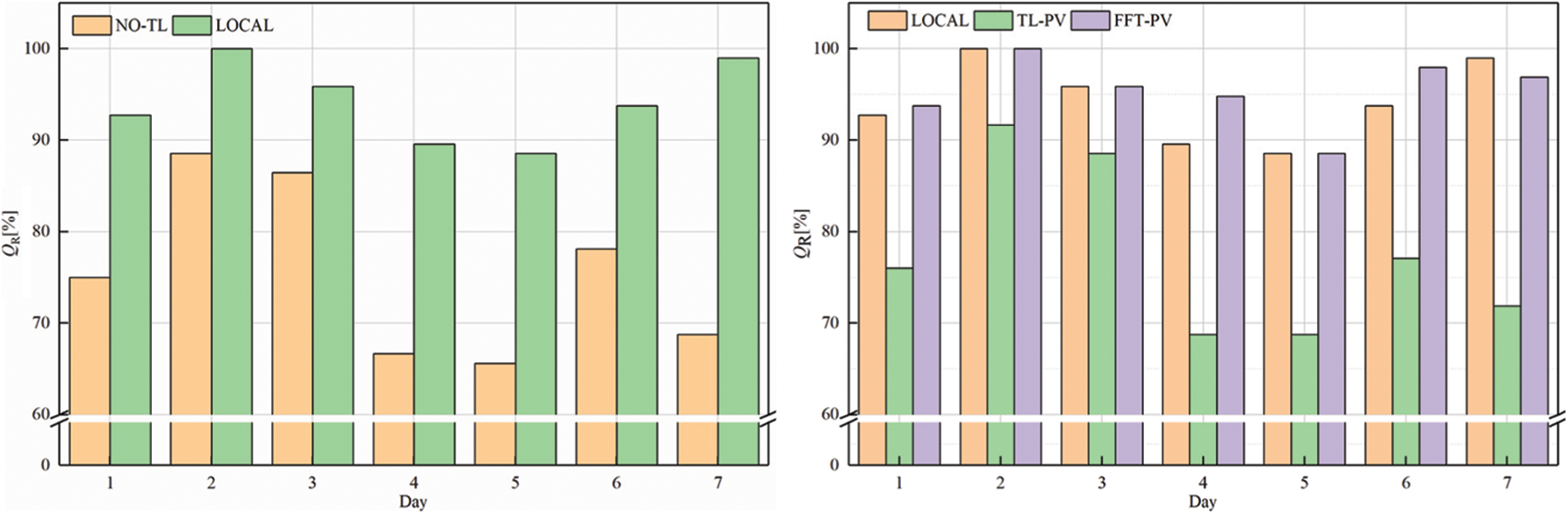
Figure 8: QR of target domain A
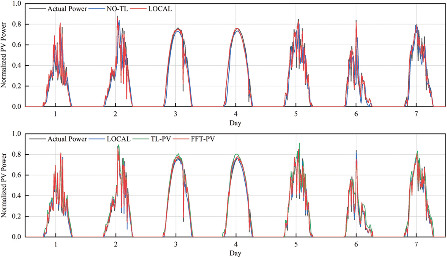
Figure 9: Comparison of PV-power predictions of the various models in target domain B
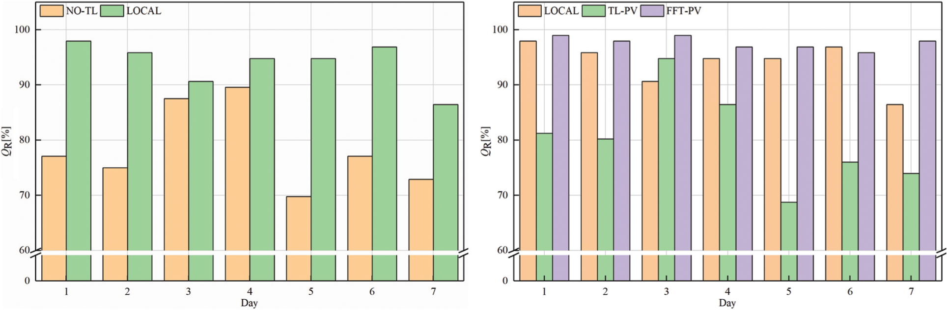
Figure 10: QR of target domain B
Comparing QR of the LOCAL model and no-TL model in target domain A shows that the qualification rate for the prediction model without TL decreases significantly, which prevents it from meeting the accuracy requirements. Moreover, the prediction model based on FFT-PV produces significantly more accurate predictions of PV power than does the traditional TL-PV model, and the prediction accuracy of the local model is similar to FFT-PV when given sufficient data.
As shown in Table 5, the indicators of FFT-PV are significantly better than those of the no-TL and TL-PV models, and the accuracy is equivalent to that of the LOCAL model. Compared with the no-TL model, the NRMSE, NMAPE, and NLAE of the FFT-PV model decrease by 23.11%, 18.17%, and 39.26%, respectively. Compared with the TL-PV model, the NRMSE, NMAPE, and NLAE of the FFT-PV model decrease by 24.29%, 18.35%, and 55.53%, respectively.
For target domain B, compared with the no-TL model, the NRMSE, NMAPE, and NLAE of the FFT-PV model decrease by 24.43%, 19.28%, and 53.06%, respectively. Compared with the TL-PV model, the NRMSE, NMAPE, and NLAE of the FFT-PV model decrease by 14.78%, 12.65%, and 44.87%, respectively. Fig. 10 shows that unstable weather conditions amplify the advantages of the FFT-PV model.
Like target domain A, the FFT-PV model of target domain B increases the prediction accuracy with respect to the no-TL and TL-PV models and suppresses overfitting.
Synthesizing target domains A and B shows that the LOCAL model uses sufficient local data for training, so the prediction accuracy is high. The no-TL model uses the target domain data to directly train the source domain model and overfits the learning of small samples, so the prediction accuracy is the worst of all models studied. The TL-PV model is not a physically accurate model, so its results are not much better than those of the no-TL model. The fluctuation range of the FFT-PV model is closest to the true range of fluctuations, and the recognition accuracy and real-time performance of the features are also better than those of the other solutions.
To summarize, the FFT-PV model based on the GRU framework proposed herein not only can be applied to different data domains to overcome the problem of insufficient local training data for newly built PV power plants but also can be widely generalized.
Based on open and shared power data, we develop herein a model to make short-term predictions of PV power based on fusion device feature transfer. The results lead to the following main conclusions:
• The feature extraction based on UMAP is clearly superior to that based on the PCA and t-SNE algorithms for processing weather datasets and accelerates the projection by balancing the global structure with the local structure. The weather feature constructed by the UMAP algorithm increases the iteration speed of the neural network.
• Taking the PV power data of Pianguan, China as the source domain label, the GRU framework with the simple structure prediction model produces an average reduction of 3%, 4%, and 5% for the NRMSE, NMAPE, and NLAE with respect to the other frameworks.
• Taking the PV power data of the Desert Knowledge Australia Solar Centre as the target domain label, we establish a fine-tuned FC layer by sharing the hidden layer and introducing regularization constraints in the feature transfer. The FFT-PV produces an average reduction of 15%, 12%, and 35% for the NRMSE, NMAPE, and NLAE with respect to the other methods, and overfitting is suppressed for target-domain training.
• of The innovation introduced by this study is the integration of transfer learning with the physical characteristics of PV-power plants. By establishing high-precision models for different PV devices and local meteorological models, and fine-tuning network parameters according to structural constraints and PV-plant features, we resolve the problems whereby new PV-power stations have insufficient data and trained prediction models are difficult to generalize for use on different PV-power stations. The proposed model enables new grid-connected PV-power plants to benefit from high-precision PV-power prediction, which increases the use of PV power and thereby contributes significantly to the goal of carbon peaking and carbon neutralization.
Acknowledgement: This research was supported by the National Natural Science Foundation of China (No. 6180802161), the Educational Commission of Liaoning Province of China (No. JZL201915401). We thank TopEdit (https://www.topeditsci.com) for its linguistic assistance during the preparation of this manuscript.
Funding Statement: The authors received no specific funding for this study.
Conflicts of Interest: The authors declare that they have no conflicts of interest to report regarding the present study.
1. Li, Z., Chen, S., Dong, W., Liu, P., Du, E. et al. (2021). Low carbon transition pathway of power sector under carbon emission constraints. Proceedings of the CSEE, 41(12), 3987–4001. DOI 10.13334/j.0258-8013.pcsee.210671. [Google Scholar] [CrossRef]
2. Faraji, J., Ketabi, A., Hashemi-Dezaki, H., Shafie-Khah, M., Catalao, J. P. (2020). Optimal day-ahead scheduling and operation of the prosumer by considering corrective actions based on very short-term load forecasting. IEEE Access, 8, 83561–83582. DOI 10.1109/ACCESS.2020.2991482. [Google Scholar] [CrossRef]
3. Das, U. K., Tey, K. S., Seyedmahmoudian, M., Mekhilef, S., Idris, M. Y. I. et al. (2018). Forecasting of photovoltaic power generation and model optimization: A review. Renewable & Sustainable Energy Reviews, 81, 912–928. DOI 10.1016/j.rser.2017.08.017. [Google Scholar] [CrossRef]
4. Ahmed, R., Sreeram, V., Mishra, Y., Arif, M. D. (2020). A review and evaluation of the state-of-the-art in PV solar power forecasting: Techniques and optimization. Renewable and Sustainable Energy Reviews, 124, 109792. DOI 10.1016/j.rser.2020.109792. [Google Scholar] [CrossRef]
5. Faraji, J., Abazari, A., Babaei, M., Muyeen, S. M., Benbouzid, M. (2020). Day-ahead optimization of prosumer considering battery depreciation and weather prediction for renewable energy sources. Applied Sciences, 10(8), 2774. DOI 10.3390/app10082774. [Google Scholar] [CrossRef]
6. Antonanzas, J., Osorio, N., Escobar, R., Urraca, R., Martinez-de-Pison, F. J. et al. (2016). Review of photovoltaic power forecasting. Solar Energy, 136, 78–111. DOI 10.1016/j.solener.2016.06.069. [Google Scholar] [CrossRef]
7. Niu, D., Wang, K., Sun, L., Wu, J., Xu, X. (2020). Short-term photovoltaic power generation forecasting based on random forest feature selection and CEEMD: A case study. Applied Soft Computing, 93, 106389. DOI 10.1016/j.asoc.2020.106389. [Google Scholar] [CrossRef]
8. Liu, L., Zhao, Y., Chang, D., Xie, J., Ma, Z. et al. (2018). Prediction of short-term PV power output and uncertainty analysis. Applied Energy, 228, 700–711. DOI 10.1016/j.apenergy.2018.06.112. [Google Scholar] [CrossRef]
9. Massaoudi, M., Chihi, I., Abu-Rub, H., Refaat, S. S., Oueslati, F. S. (2021). Convergence of photovoltaic power forecasting and deep learning: State-of-art review. IEEE Access, 9, 136593–136615. DOI 10.1109/ACCESS.2021.3117004. [Google Scholar] [CrossRef]
10. Chu, Y., Urquhart, B., Gohari, S. M., Pedro, H. T., Kleissl, J. et al. (2015). Short-term reforecasting of power output from a 48 MWe solar PV plant. Solar Energy, 112, 68–77. DOI 10.1016/j.solener.2014.11.017. [Google Scholar] [CrossRef]
11. Nie, Y., Sun, Y., Chen, Y., Orsini, R., Brandt, A. (2020). PV power output prediction from sky images using convolutional neural network: The comparison of sky-condition-specific sub-models and an end-to-end model. Journal of Renewable and Sustainable Energy, 12(4), 46101. DOI 10.1063/5.0014016. [Google Scholar] [CrossRef]
12. Faraji, J., Ketabi, A., Hashemi-Dezaki, H., Shafie-Khah, M., Catalão, J. P. (2020). Optimal day-ahead self-scheduling and operation of prosumer microgrids using hybrid machine learning-based weather and load forecasting. IEEE Access, 8, 157284–157305. DOI 10.1109/ACCESS.2020.3019562. [Google Scholar] [CrossRef]
13. Wang, F., Xuan, Z., Zhen, Z., Li, K., Wang, T. et al. (2020). A Day-ahead PV power forecasting method based on LSTM-RNN model and time correlation modification under partial daily pattern prediction framework. Energy Conversion and Management, 212, 112766. DOI 10.1016/j.enconman.2020.112766. [Google Scholar] [CrossRef]
14. Gao, M., Li, J., Hong, F., Long, D. (2019). Day-ahead power forecasting in a large-scale photovoltaic plant based on weather classification using LSTM. Energy, 187, 115838. DOI 10.1016/j.energy.2019.07.168. [Google Scholar] [CrossRef]
15. Adar, M., Najih, Y., Gouskir, M., Chebak, A., Mabrouki, M. et al. (2020). Three PV plants performance analysis using the principal component analysis method. Energy, 207, 118315. DOI 10.1016/j.energy.2020.118315. [Google Scholar] [CrossRef]
16. Lee, H., Lee, J. G., Kim, N. W., Lee, B. T. (2021). Model-agnostic online forecasting for PV power output. IET Renewable Power Generation, 15(15), 3539–3551. DOI 10.1049/rpg2.12243. [Google Scholar] [CrossRef]
17. Wang, F., Zhang, Z., Liu, C., Yu, Y., Pang, S. et al. (2019). Generative adversarial networks and convolutional neural networks based weather classification model for day ahead short-term photovoltaic power forecasting. Energy Conversion and Management, 181, 443–462. DOI 10.1016/j.enconman.2018.11.074. [Google Scholar] [CrossRef]
18. Zhao, Y., Xia, S., Zhang, J., Hu, Y., Wu, M. (2021). Effect of the digital transformation of power system on renewable energy utilization in China. IEEE Access, 9, 96201–96209. DOI 10.1109/ACCESS.2021.3094317. [Google Scholar] [CrossRef]
19. Dolara, A., Leva, S., Manzolini, G. (2015). Comparison of different physical models for PV power output prediction. Solar Energy, 119, 83–99. DOI 10.1016/j.solener.2015.06.017. [Google Scholar] [CrossRef]
20. Zhang, L., Chen, Z., Zhang, H., Ma, Z., Cao, B. et al. (2020). Accurate study and evaluation of small PV power generation system based on specific geographical location. Energy Engineering, 117(6), 453–470. DOI 10.32604/EE.2020.013276. [Google Scholar] [CrossRef]
21. Yuan, W., Ji, J., Li, Z., Zhou, F., Ren, X. et al. (2018). Comparison study of the performance of two kinds of photovoltaic/thermal(PV/T) systems and a PV module at high ambient temperature. Energy, 148, 1153–1161. DOI 10.1016/j.energy.2018.01.121. [Google Scholar] [CrossRef]
22. Kurnik, J., Jankovec, M., Brecl, K., Topic, M. (2011). Outdoor testing of PV module temperature and performance under different mounting and operational conditions. Solar Energy Materials and Solar Cells, 95(1), 373–376. DOI 10.1016/j.solmat.2010.04.022. [Google Scholar] [CrossRef]
23. Walwil, H. M., Mukhaimer, A., Al-Sulaiman, F. A., Said, S. A. (2017). Comparative studies of encapsulation and glass surface modification impacts on PV performance in a desert climate. Solar Energy, 142, 288–298. DOI 10.1016/j.solener.2016.12.020. [Google Scholar] [CrossRef]
24. Holmgren, W. F., Lorenzo, A. T., Hansen, C. (2017). A comparison of PV power forecasts using PVLib-Python. IEEE 44th Photovoltaic Specialist Conference (PVSC), pp. 1127–1131. Washington DC, USA. DOI 10.1109/PVSC.2017.8366724. [Google Scholar] [CrossRef]
25. Olalla, C., Hasan, M., Deline, C., Maksimović, D. (2018). Mitigation of hot-spots in photovoltaic systems using distributed power electronics. Energies, 11(4), 726. DOI 10.3390/en11040726. [Google Scholar] [CrossRef]
26. Jordan, D. C., Silverman, T. J., Sekulic, B., Kurtz, S. R. (2017). PV degradation curves: Non-linearities and failure modes. Progress in Photovoltaics, 25(7), 583–591. DOI 10.1002/pip.2835. [Google Scholar] [CrossRef]
27. Bhallamudi, R., Kumarasamy, S., Sundarabalan, C. K. (2021). Effect of dust and shadow on performance of solar photovoltaic modules: Experimental analysis. Energy Engineering, 118(6), 1827–1838. DOI 10.32604/EE.2021.016798. [Google Scholar] [CrossRef]
28. Maitanova, N., Telle, J. S., Hanke, B., Grottke, M., Schmidt, T. et al. (2020). A machine learning approach to Low-cost photovoltaic power prediction based on publicly available weather reports. Energies, 13(3), 735. DOI 10.3390/en13030735. [Google Scholar] [CrossRef]
29. Singh, P., Dhiman, G. (2018). Uncertainty representation using fuzzy-entropy approach: Special application in remotely sensed high-resolution satellite images (RSHRSIs). Applied Soft Computing, 72, 121–139. DOI 10.1016/j.asoc.2018.07.038. [Google Scholar] [CrossRef]
30. McInnes, L., Healy, J., Melville, J. (2020). UMAP: Uniform manifold approximation and projection for dimension reduction. https://arxiv.org/abs/1802.03426. [Google Scholar]
31. Keskar, N. S., Socher, R. (2017). Improving generalization performance by switching from adam to sgd. https://arxiv.org/abs/1712.07628. [Google Scholar]
32. Gao, S., Huang, Y., Zhang, S., Han, J., Wang, G. et al. (2020). Short-term runoff prediction with GRU and LSTM networks without requiring time step optimization during sample generation. Journal of Hydrology, 589, 125188. DOI 10.1016/j.jhydrol.2020.125188. [Google Scholar] [CrossRef]
33. Ghazi, M. M., Yanikoglu, B., Aptoula, E. (2017). Plant identification using deep neural networks via optimization of transfer learning parameters. Neurocomputing, 235, 228–235. DOI 10.1016/j.neucom.2017.01.018. [Google Scholar] [CrossRef]
34. Tan, Y., Zhao, G. (2020). Transfer learning with long short-term memory network for state-of-health prediction of lithium-ion batteries. IEEE Transactions on Industrial Electronics, 67(10), 8723–8731. DOI 10.1109/TIE.2019.2946551. [Google Scholar] [CrossRef]
35. Iiduka, H., Kobayashi, Y. (2020). Training deep neural networks using conjugate gradient-like methods. Electronics, 9(11), 1809. DOI 10.3390/electronics9111809. [Google Scholar] [CrossRef]
36. Raza, M. Q., Nadarajah, M., Ekanayake, C. (2016). On recent advances in PV output power forecast. Solar Energy, 136, 125–144. DOI 10.1016/j.solener.2016.06.073. [Google Scholar] [CrossRef]
 | This work is licensed under a Creative Commons Attribution 4.0 International License, which permits unrestricted use, distribution, and reproduction in any medium, provided the original work is properly cited. |