Energy Engineering

---

DOI: 10.32604/ee.2022.019556

ARTICLE

Production Dynamic Prediction Method of Waterflooding Reservoir Based on Deep Convolution Generative Adversarial Network (DC-GAN)

Liyuan Xin1,2,3, Xiang Rao1,2,3,*, Xiaoyin Peng1,2,3, Yunfeng Xu1,2,3 and Jiating Chen1,2,3

1Cooperative Innovation Center of Unconventional Oil and Gas (Ministry of Education & Hubei Province), Yangtze University, Wuhan, 430100, China
2Key Laboratory of Drilling and Production Engineering for Oil and Gas, Wuhan, 430100, China
3School of Petroleum Engineering, Yangtze University, Wuhan, 430100, China
*Corresponding Author: Xiang Rao. Email: raoxiang0103@163.com
Received: 29 September 2021; Accepted: 22 December 2021

1  Introduction

The development of new methods for oilfield production optimization has been an urgent problem that should be solved in the process of oil production. The layout of injection and production wells in the oilfield is the key to the optimization of reservoir development. The well location deployment and well location optimization are directly related to the final development effect of the oilfield. Zhou et al. [1] took Jilin’s two wells ultra-low permeability oilfield as the research object, using numerical simulation software to simulate and predict the diamond well location and rectangular well location of the reservoir, selecting the best well location. Cao et al. [2] selected ultra-low permeability reservoirs in Changqing’s Oilfield as the research object, through the adjustment of rhombic inverted nine-point injection-production well location in this block, the feasibility analysis of well location conversion and well location refinement was carried out, and the oil recovery rate was optimized and enhanced. According to the characteristics of ultra-low permeability and tight reservoirs in Ordos Basin, Zhao et al. [3] used the numerical simulation software to study the horizontal well and well location form. Zhang et al. [4] conducted low permeability reservoir fracturing horizontal well pattern optimization. Cai et al. [5] used numerical simulation and reservoir engineering methods, studied the horizontal well and vertical well joint well pattern type and well spacing optimization. Zhao et al. [6] combined seepage theory with reservoir numerical simulation, derived the productivity formula of staggered well pattern in low permeability reservoir, obtained the relationship curve between well pattern form factor and dimensionless production. There are also other excellent studies. combining numerical simulation with well location optimization [7–14].

However, we know that the basis of reservoir production optimization is to be able to make rapid production dynamic prediction based on well location deployment, to obtain the optimal production mode and well layout mode in oilfield development planning [15,16]. The geological modeling and simulation calculation process of the traditional numerical simulation method is very time-consuming, and most optimization algorithms need to call numerical simulation tools repeatedly and iteratively, which leads to the optimization efficiency being greatly reduced. Therefore, it is of great significance to establish the rapid prediction model of water flooding reservoir production dynamic under different well location deployment by intelligent method for well pattern optimization. With the rapid development of artificial intelligence technology, an intelligent optimization algorithm is gradually applied to the field of reservoir development and has achieved a lot of remarkable results [17–23]. Gu et al. [24,25] proposed a new method of remaining oil distribution prediction based on machine learning. According to the existing reservoir numerical simulation results, the remaining oil distribution prediction training was carried out under the model of support vector machine and long-term and short-term memory neural network, and the remaining oil prediction model was built to accomplish the purpose of simple and rapid prediction of remaining oil in oil plane. Gu et al. [26] proposed a prediction model based on an artificial neural network (ANN) for the problems existing in the traditional water flooding reservoir production prediction method. The model selected the Bayesian regularization algorithm to train the model and used the nonlinear autoregressive network with external input as the structure of the oil production prediction model. Negash et al. [27] used the embedded discrete fracture model to generate sample data for the development of water injection huff and puff in fractured horizontal wells, and based on the artificial neural network model, a proxy model for production performances prediction of the fractured horizontal well is constructed. Rao et al. [28] established the production prediction model of extra-high water cut stage of water flooding reservoirs. Although ANN has been widely used to conduct the proxy model for production prediction, the slow convergence speed and low prediction accuracy also exist in ANN.

In 2020, Wang et al. [29] proposed an automatic well test interpretation method for the radial composite reservoir based on a convolutional neural network (CNN). This article points out and verifies that CNN can effectively avoid data overfitting, quickly and accurately obtain obvious feature optimization networks through large data scale, and improve the accuracy of the model prediction. In the same year, Li et al. [30] proposed the prediction of gas channeling direction based on DC-GAN. The DC-GAN was used to establish the dynamic mapping of permeability field and gas saturation distribution. The research shows that the DC-GAN has good performance in extracting permeability characteristics, and has an excellent performance in the mapping relationship between input and output of high-dimensional model [31–33]. The deep convolution network is introduced into the generative adversarial network, which can not only effectively extract features, but also quickly converge data, and optimize the training model [34–38]. In addition, we also researched a large number of references to verify the powerful potential of DC-GAN [39–43].

According to the above literature research, the authors found that the DC-GAN method can effectively avoid data over-fitting, quickly and accurately extract data features, and has good performance in dynamic prediction, author decided to use the DC-GAN model to predict the dynamic production of water flooding reservoirs. Based on the improved U-Net framework [44], the dynamic mapping relationship between the well location deployment and the output oil saturation under waterflooding was established, and the proxy model that can quickly predict the production performance of water flooding reservoirs was constructed, and the accuracy and efficiency of the dynamic prediction about oil saturation under waterflooding reservoirs were significantly improved.

2  Research Methodology

2.1 Data Preparation

This paper aims to establish a prediction model based on DC-GAN to reflect the dynamic mapping relationship between well location deployment and output oil saturation in waterflooding reservoirs. Due to the production parameters such as well location deployment and geological parameters such as oil saturation being mostly established on the whole reservoir scale, there will be a large amount of calculation data and an uncertain geological model. Therefore, the methods used ANN and other machine learning methods that directly train the data itself are difficult to obtain good training results and cause the network model structure to be extremely large and complex. Therefore, the idea of this paper is to convert these two kinds of data into an image. Through DC-GAN, the features of input parameters are extracted, and the mapping relationship is established, then the proxy model is optimized combined with GAN.

The quality of the sample is directly related to the accuracy and stability of the neural network model. Therefore, this paper uses the traditional numerical simulator (MRST) for input image [45], that this simulator is a famous open simulator developed by the Norwegian Institute of science, technology and industry, and SINTEF, it can effectively reduce the difficulty of the input image and improve the efficiency, and ensure the efficiency and accuracy of the preprocessing. Basic physical properties used in this numerical example Table 1 and the data preprocessing process are shown in Fig. 1.

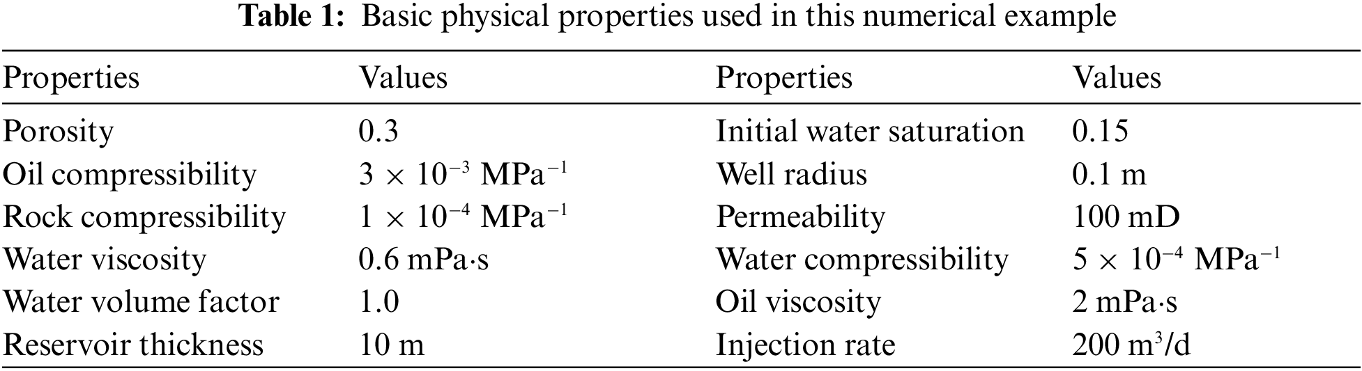
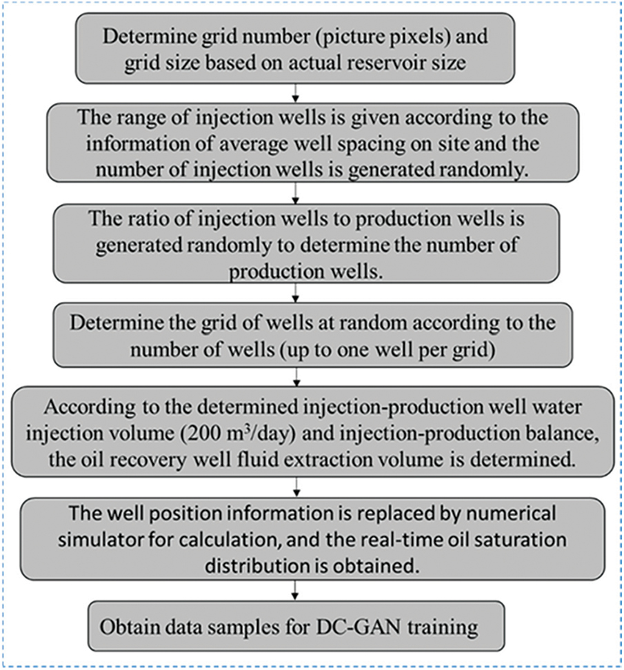
Figure 1: Data generation pre-processing flow

Input image: According to the actual reservoir size, the grid number (pixel point of the image) and grid size are determined. The range of the number of water injection wells is given according to the average well spacing information on the site, and the number of water injection wells is randomly generated. The number of production wells is determined according to the ratio of randomly generated water injection wells to the number of production wells. Then, the grid position of each well is randomly determined according to the number of wells, and it is required that each grid has at most one well (we set 1 as water injection wells, −1 as production wells, 0 as empty wells, and the number of production wells should be much larger than that of water injection wells according to the actual production). Finally, the corresponding well location deployment picture (Fig. 2a) is obtained. According to the determined injection rate of water injection wells (200 square/day) and the injection-production balance, the liquid production rate of production wells is determined, and the information of each well location is taken into the numerical simulator for calculation,

Output image: As mentioned above, we use the traditional numerical simulation to obtain the real-time oil saturation map (as shown in Fig. 2b) in the case of the corresponding well location deployment map (input image) and the known geological parameters. We generally believe that the injection-production balance of water-drive reservoirs, so the surface pressure changes little, that is, the pore volume changes little. Therefore, the cumulative oil production of the whole block can be estimated according to the distribution of oil saturation. The formula is as follows:

∑i=1i=n[(Soi(0)−Soi(n))ViΦi](1)

where: Soi refers to oil saturation, Vi refers to pore volume, and Φi refers to the porosity.

This oil saturation map is used as the output image to verify the output image of the sample training of the input well deployment map through the DC-GAN.

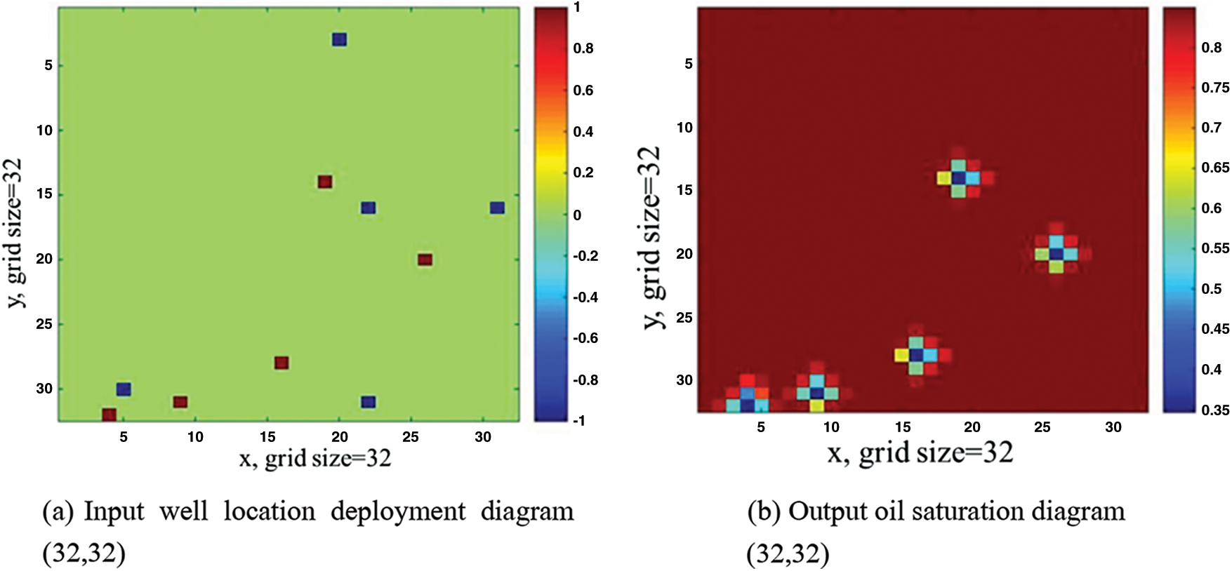
Figure 2: Result diagram

2.2 Deep Convolution Generative Adversarial Network Model (DC-GAN)

2.2.1 Generative Adversarial Network (GAN)

A generative adversarial network (GAN) is a network model of deep learning. It can force the generated image to be almost indistinguishable from the real image in statistics, to generate quite realistic synthetic images and predict the required data with new data. The GAN is composed of the generator (G) and discriminator (D). The generator takes a random vector as the input data and decodes it into a synthetic image. The image is introduced into the discriminator for discrimination. The discriminator takes an image as the input and predicts whether the image is a real image from the training set or a false image of the generator. In this paper, the input of the generator is directly the well location deployment picture, and the discriminator determines whether the input picture is the real oil saturation picture or the picture generated by the generator. The purpose of the generator network can deceive the discriminator network. Therefore, with the operation of training, it can gradually generate more and more realistic images, that is, images that can not be distinguished from real images. At the same time, the discriminator is constantly adapting to the gradually improved ability of the generator and improving its ability, which is the mutual competition between the generator (G) and the discriminator (D), also known as confrontation training.

The generator G(x) is used to represent the mapping relationship G(x):X->Y of the input image, and the discriminator (D) is used to identify whether the data comes from the model D(y) generated by the generator or the obtained model D(G(x)). D attempts to maximize the probability of its correct classification of true and false (log (x)), and G attempts to minimize D will predict that its output is false (log(1−D(G(x)))), its loss function is L(G,D).

The formula of GAN is:

G=argminGmaxDV(G,D)(2)

The distance between the two distributions is measured by V(G,D). The greater the V, the greater the distance, and the greater the difference between the two distributions; D is to make the distance as far as possible; G is to make the distance as small as possible, to form a confrontation:

V=Ex∼Pdata×[lgD(x)]+Ex∼PG[lg(1−D(x)](3)

where Ex∼Pdata and Ex∼PG represent solving expectations from real data and expectations from the proxy model.

The loss function is expressed as:

L(G,D)=1m∑i=1mlgD(Xi)+1m∑i=1mlg(1−D(G(zi)))(4)

In adversarial training, we continuously improve the ability of generators and discriminators by iterative computation. The network construction idea of our GAN is shown in Fig. 3 below.

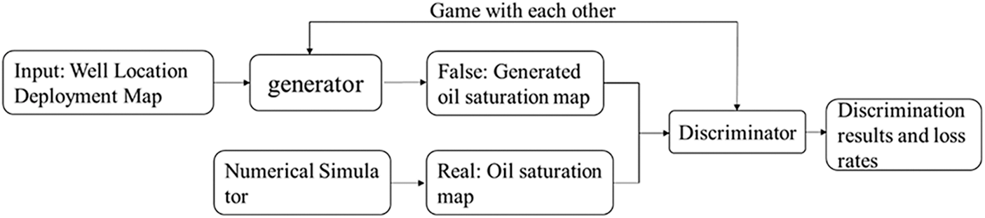
Figure 3: GAN network construction diagram

2.2.2 Convolutional Neural Network (CNN)

A convolutional neural network (CNN) is a feedforward neural network, which is composed of the input layer, convolution layer, pooling layer, and full connection layer. The convolution layer is the core layer of constructing a convolutional neural network, which produces most of the computation in the network. The convolution layer can have several, and the main purpose is to detect features. The pooling layer is generally sandwiched in the middle of the convolution layer, which is used to compress the amount of data and parameters and to greatly reduce the order of magnitude, to avoid the phenomenon of overfitting. The activation function follows the convolution layer, which adds nonlinearity to the network and improves the performance and generalization of the neural network. CNN can effectively reduce the dimension of big data pictures to a small amount of data, and can effectively retain picture features. At the same time, CNN has translation invariance. It can make efficient use of data when processing pictures and can obtain generalized data representation with only a few training samples. Therefore, the convolutional neural network has the ability to efficient and stable feature extraction.

The input and convolution kernel of the convolution layer is usually multi-dimensional array data. Convolution operation can be regarded as the process of convolution kernel sliding on the input data. Convolution operation reads the sum of pixels in each region through the movement of convolution, inputs feature map, extracts blocks, and applies the same transformation to all these blocks to generate an output feature map. Unlike regular networks, the neurons in each layer of a convolution neural network are arranged in three dimensions: width, height, and depth, and the depth in the convolution neural network grid refer to the number of layers of the network. The dimension of the input well location deployment map in this paper is (width, height, and depth) We can see that the neurons in the layer connect only to a small area in the previous layer, not to a full connection, as shown in Fig. 4.

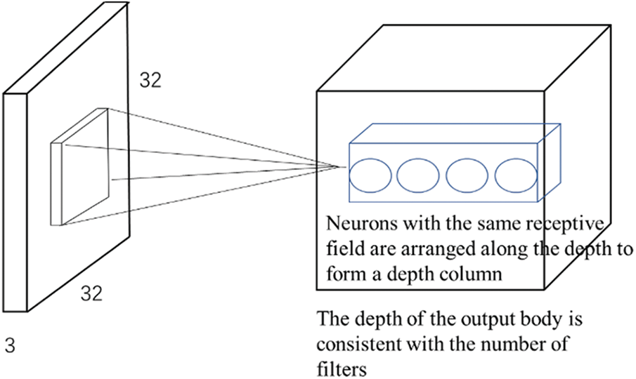
Figure 4: Convolutional neural network field of view connection graph

2.2.3 Deep Convolution Generative Adversarial Network Model (DC-GAN)

The structure of DC-GAN and GAN is similar, GAN is difficult to train mapping relationships between images directly, while CNN is an effective way to process images, so DC-GAN adds a means to process images within the framework of GAN, thus enabling adversarial neural networks to train mapping relationships between images effectively, so it transforms the multi-layer perceptron of the original GAN generation model G and the discriminant model D into two convolutional neural networks. In the process of constructing the generator, the deep convolutional network is used to replace the traditional nonlinear mapping. By inputting multidimensional vector parameters and through a series of convolution operations, the well location deployment map is convoluted, offset, normalized, activated, and other steps to form the middle parameter feature image. At the same time, we use deconvolution network operation for up-sampling to form the output oil saturation map after multi-dimensional mapping and use the normal distribution to sample points in the potential space, to improve randomness and further improve the robustness of GAN training.

The network model in the generator is constructed based on an improved U-Net framework (as shown in Fig. 5). Using dropout in the discriminator to reduce neuronal connections and avoid overfitting, generally speaking, the sparse gradient will hinder the training of GAN, and the maximum pooling operation and ReLU activation function will result in sparse gradient, so we use step convolution instead of the maximum pooling layer for upsampling, the generator hide layer uses ReLU, the last layer uses tanh as the activation function, and the D hide layer uses LeakyReLU layer to replace ReLU activation. The last layer uses softmax as the activation function. LeakyReLU is similar to ReLU, but it allows a smaller negative activation value, thereby relaxing the sparsity limitation.

We use Pytorch to draw several common activation functions (Fig. 2 for details). Our innovation is that the input sample changes directly from the original noise to the well location deployment map, which simplifies the steps and improves the calculation rate. At the same time, the input sample of the generator changes from the original random vector to the feature vector output by the convolution layer mentioned above, and the new oil saturation map is predicted according to the characteristics of the well location deployment map.

We introduce a deconvolution layer in the model. The size of the deconvolution layer corresponds to the size of the connected convolution layer. The convolution parameters are the same. The left side extracts the characteristics of the well location deployment map by convolution, and the right side obtains the real oil saturation information through the deconvolution layer. The left input dynamic well location deployment map, the right output oil saturation map of water drive, the generator transforms image to image, and the discriminator is similar to a classifier, giving the probability of the real data of the generator output data, then they are confronted and trained. Only in this way, the trained generator model can generate the corresponding output data according to the input samples provided, rather than the traditional adversarial neural network, which is just to copy a type of image to achieve the purpose of predicting saturation.

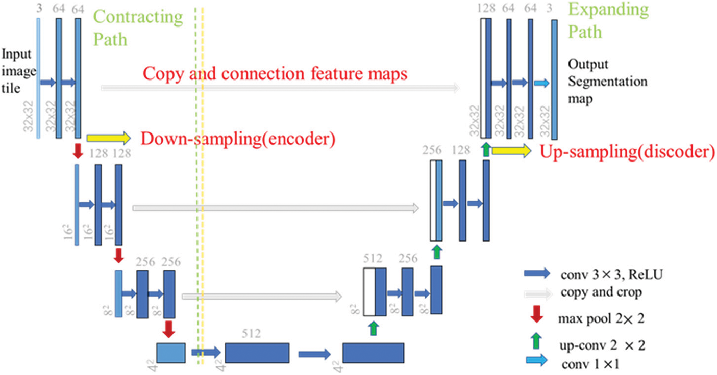
Figure 5: U-Net framework

The same points: (1) The ‘U’ structure of the U-Net framework is adopted, and the blue box is represented as a multi-channel feature map. During the down-sampling, each module has two effective convolutions and one maximum pooling calculation. The convolution kernel of the convolution layer is 3 × 3, and the convolution kernel of the maximum pooling layer is 2 × 2. In the up-sampling, each module performs one deconvolution and two convolution networks, and the convolution kernel of the deconvolution layer is 2 × 2.

Differences: (1) The U-Net framework does not use padding for boundary nulling when performing convolution operations, but in this paper, we use padding for boundary nulling to ensure that the size of the output feature graph remains unchanged.

(1) ReLU: Rectified Linear Unit from Fig. 6c, it can be seen that the value greater than 0 is not affected by this function, and the value less than 0 is returned to 0 by this activation function: ReLU(x) = max(0, x). The ReLU converges faster than the Sigmoid/Tanh function and has no exponential operation, requiring a small amount of computation, where the ReLU function sets all negatives to zero.

(2) LeakyReLU: It is an improved version of ReLU, which solves the necrosis problem of ReLU and uses a small probability at the time, that is x<0, it is also involved in gradient descent.

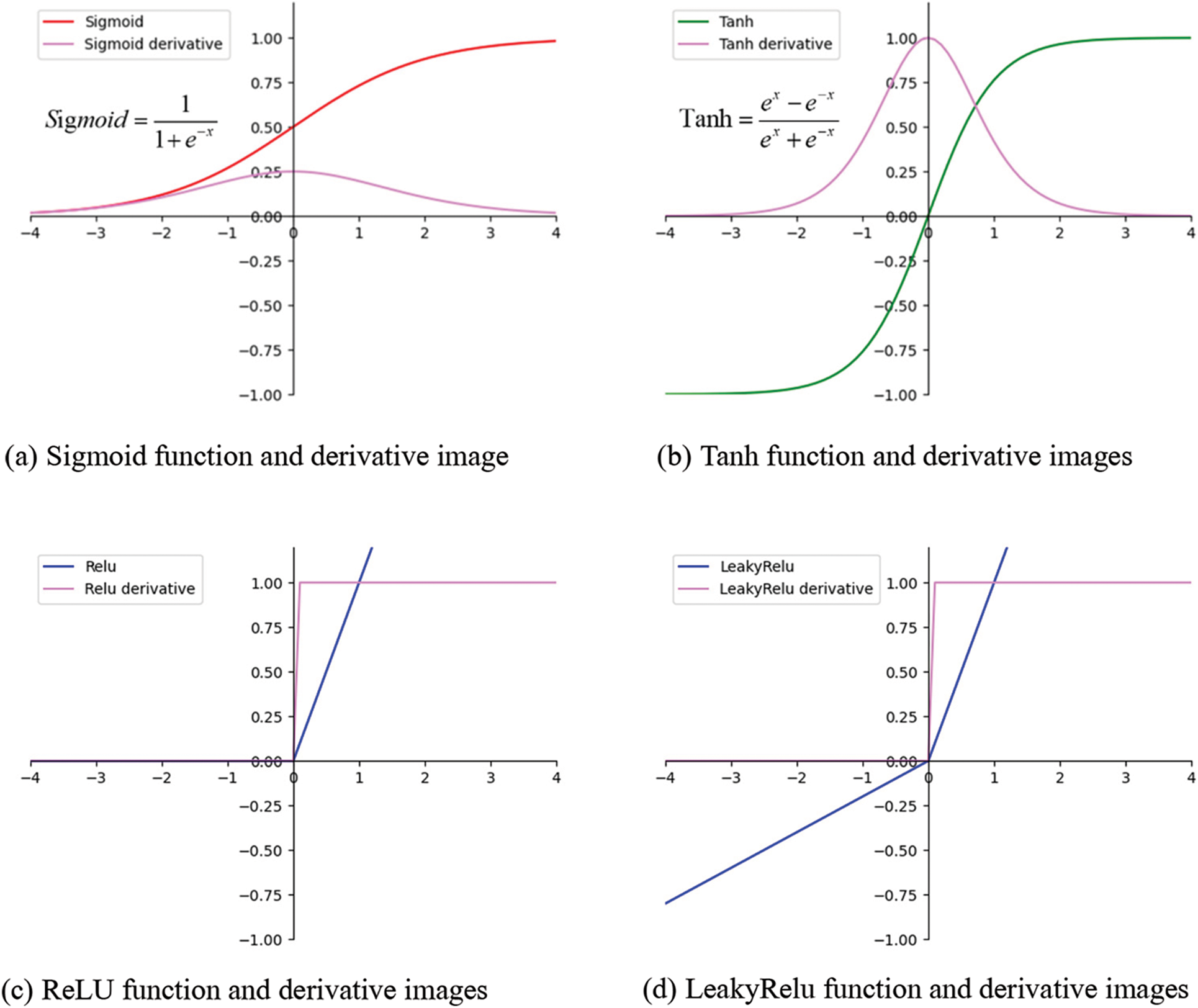
Figure 6: Images of four commonly used activation functions and derivatives

3  Training Results and Discussion

3.1 Comparison and Evaluation of Training Results

We use the traditional numerical simulator to generate input well location deployment and output oil saturation samples. According to the technique of [46], which had compared the suitable number of image samples. We take the samples at five times points, respectively, 60, 120, 180, 240, 300 days, we each time the amount of data for 6000 samples. The reservoir model is of injection-production balance, and well locations are stochastically generated. The true oil saturation map (generated by the numerical simulator) is compared with the “false” oil saturation map generated by the DC-GAN model to verify the accuracy of the model, as shown in Fig. 7.

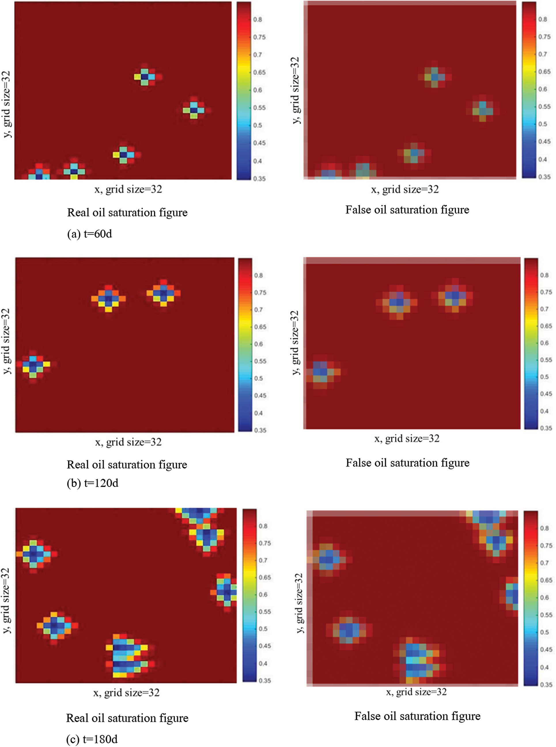
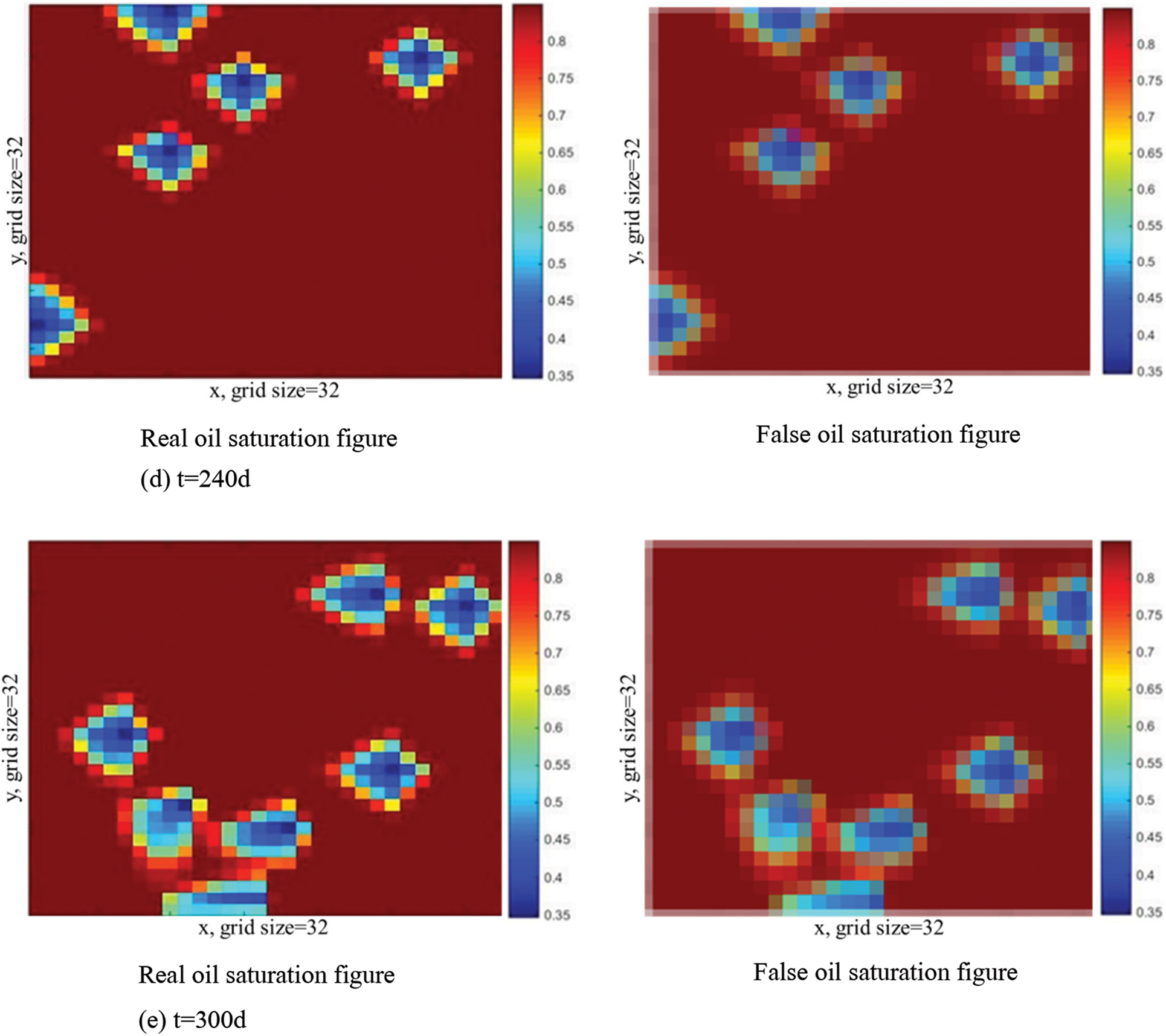
Figure 7: Comparison of true and false oil saturation at 5 moments. (a) t = 60 d; (b) t = 120 d; (c) t = 180 d; (d) t = 240 d and (e) t = 300 d

According to the oil saturation samples at five times in Fig. 3, we compared the image generation speed between the numerical simulator and the DC-GAN proxy model. The comparison is shown in Table 2.

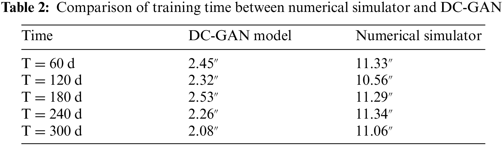
The results show that the training speed of the DC-GAN proxy model is faster than the traditional numerical simulator, it is worth noting that this is still the case of a small number of grids when the reservoir numerical model has a large number of grids, the proxy model in this paper will be more obvious to reduce the computational time. To some extent, it shows that the DC-GAN proxy model has fast training speed and great development potential. It is an efficient intelligent algorithm.

At the same time, we take the training of samples at 60 days as an example to show the data changes of generator and discriminator loss rate during DC-GAN training, as shown in Table 3. The generator functions as close as possible to the real sample generated by the DC-GAN model, that is, the closer D(G(x)) is to 1, the better. The role of the discriminator is to make D(y) as close as 1 and D(G(x)) as close as 0, However, whether the real sample or the generated sample, when the probability of the discriminator D(y) is 0.5, the state is the most ideal, it is impossible to distinguish whether the sample comes from the real sample or the generated sample.

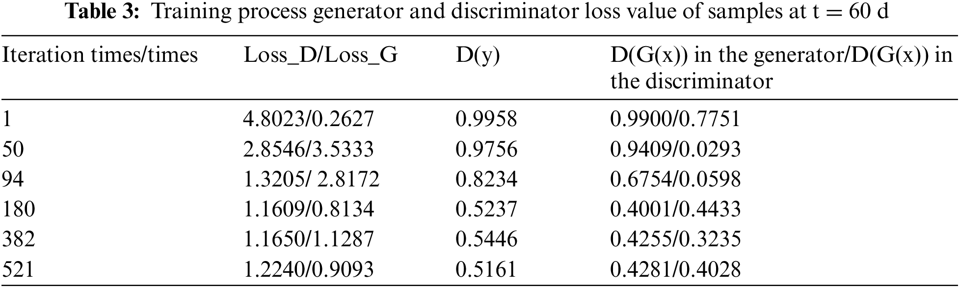
As shown in Table 3, we take the number of iterations six times and find that with the increase of the number of iterations, the loss rate of generator D and discriminator G gradually decreases, while D(y) is used to judge whether data comes from a real model or DC-GAN proxy model, so it is closer and closer to 0.5, which it is best. The generator functions as close as possible to the real sample generated by the DC-GAN model, that is, the closer D(G(x)) is to 1, the better. D(G(x)) in the generator and discriminator is closer to 0.5, indicating that the stability of the model is gradually enhanced.

The relationship between training loss values and time obtained from training for DC-GAN is shown in Fig. 8. The relationship between training loss values and the number of iterations under different production times is analyzed. To better observe the state of iteration reaching equilibrium, we set the maximum number of iterations for 3000 times at different times. Each training includes an independent training process for the generator and the discriminator.

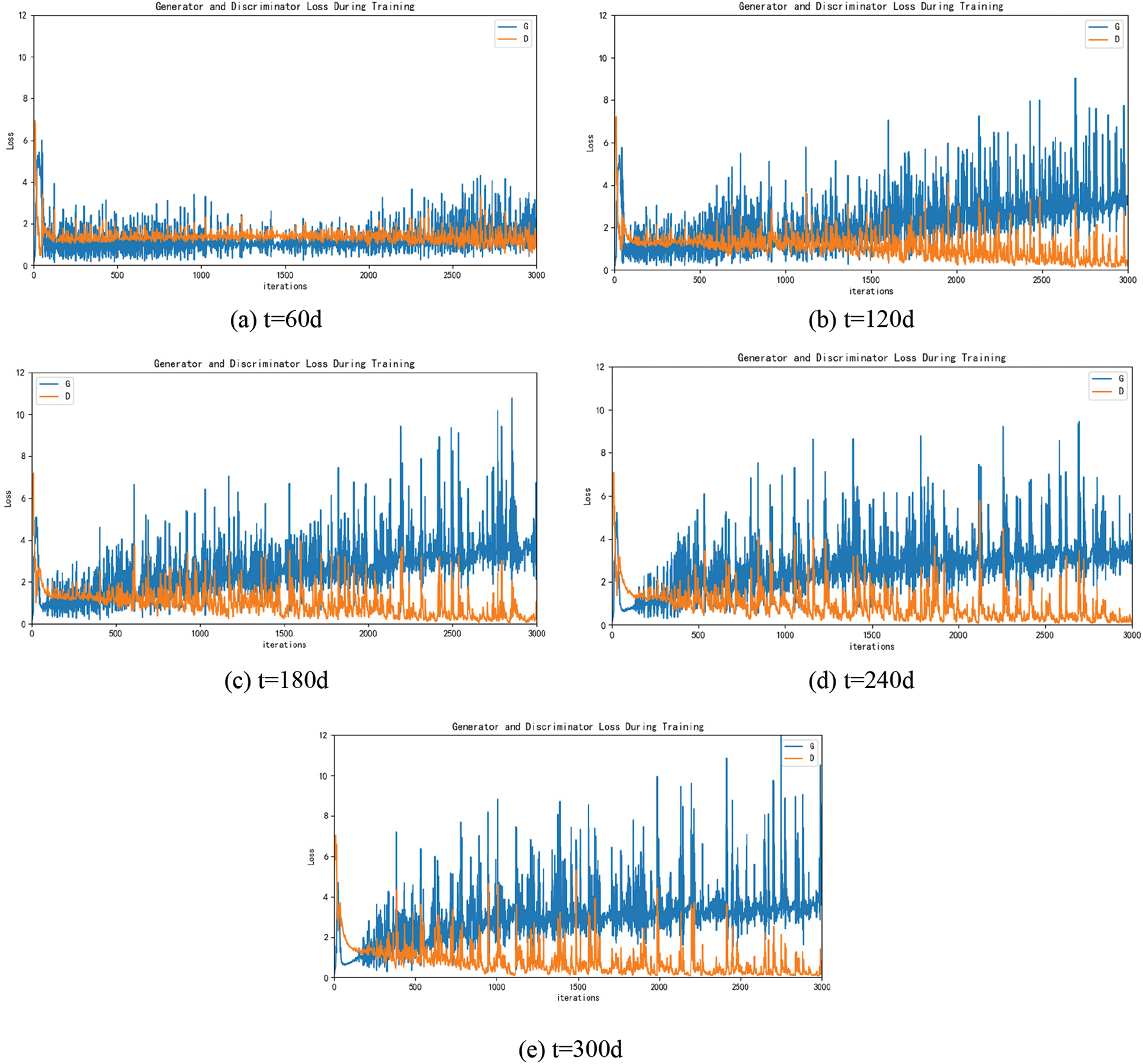
Figure 8: DC-GAN training process at different time (a) t = 60 d; (b) t = 120 d; (c) t = 180 d; (d) t = 240 d and (e) t = 300 d

Obviously, for most models, the model can reach the Nash equilibrium state and the accuracy of the model reach equilibrium before 300 training iterations. In the model of 300 days of production, oil saturation is more complex and changeable due to the distribution pattern, and water breakthrough in most of the production wells. The characteristic parameters are more complex than those before, which requires a lot of training time to reach equilibrium.

3.2 Image Cosine Similarity

For two vectors, we can imagine them as two lines in space, starting from the origin ([0, 0, …]) and pointing in different directions. There is an angle between the two lines. If the angle is 0 degrees, it means the same direction and the line overlap. If the angle is 90 degrees, that means forming a right angle, the direction is completely different. If the angle is 180 degrees, that means the opposite direction. Therefore, we can judge the similarity of vectors by the angle. The smaller the angle is, the more similar it represents.

Assuming A and B are two n-dimensional vectors, A is [A1, A2,…, A n], B is [B1, B2,…, Bn], then the cosine of the angle θ between A and B equals

similarty=cosA⋅B∥A∥∥B∥=∑i=1nAi×Bi∑i=1n(Ai)2×∑i=1n(Bi)2

The closer the cosine value is to 1, the closer the angle is to 0 degree, that is, the more similar the two vectors are, which is called cosine similarity. By comparing the true and “false” (generated) maps of six groups about oil saturation distribution, the corresponding cosine similarity values are obtained, as shown in Table 4.

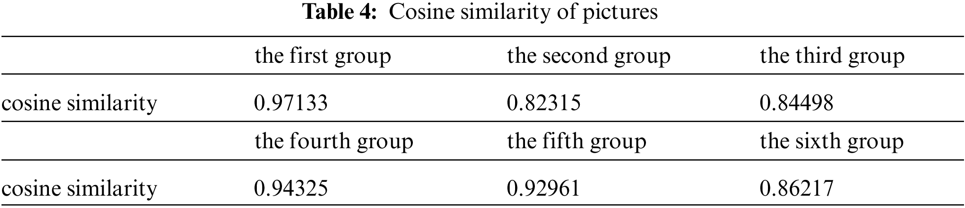
The numbers in the table represent the cosine similarity between the two images, and it can be seen that the similarity between the images is generally above 80% and even up to 97%, which shows the high accuracy of the training model.

Under the condition of the same geological parameters, according to the same well location deployment map, taking 300 days as an example, the oil saturation map obtained by DC-GAN model training is drawn, and compared with the oil saturation map obtained by reservoir numerical simulator, as shown in Fig. 9. According to the similarity of images, the training results are consistent with the traditional digital simulation results. The oil saturation map based on DC-GAN model training can accurately extract the variation characteristics of the oil saturation map, and can effectively predict the dynamic mapping relationship between well location deployment and oil saturation in water flooding reservoirs, reflecting the reliability of the DC-GAN model.

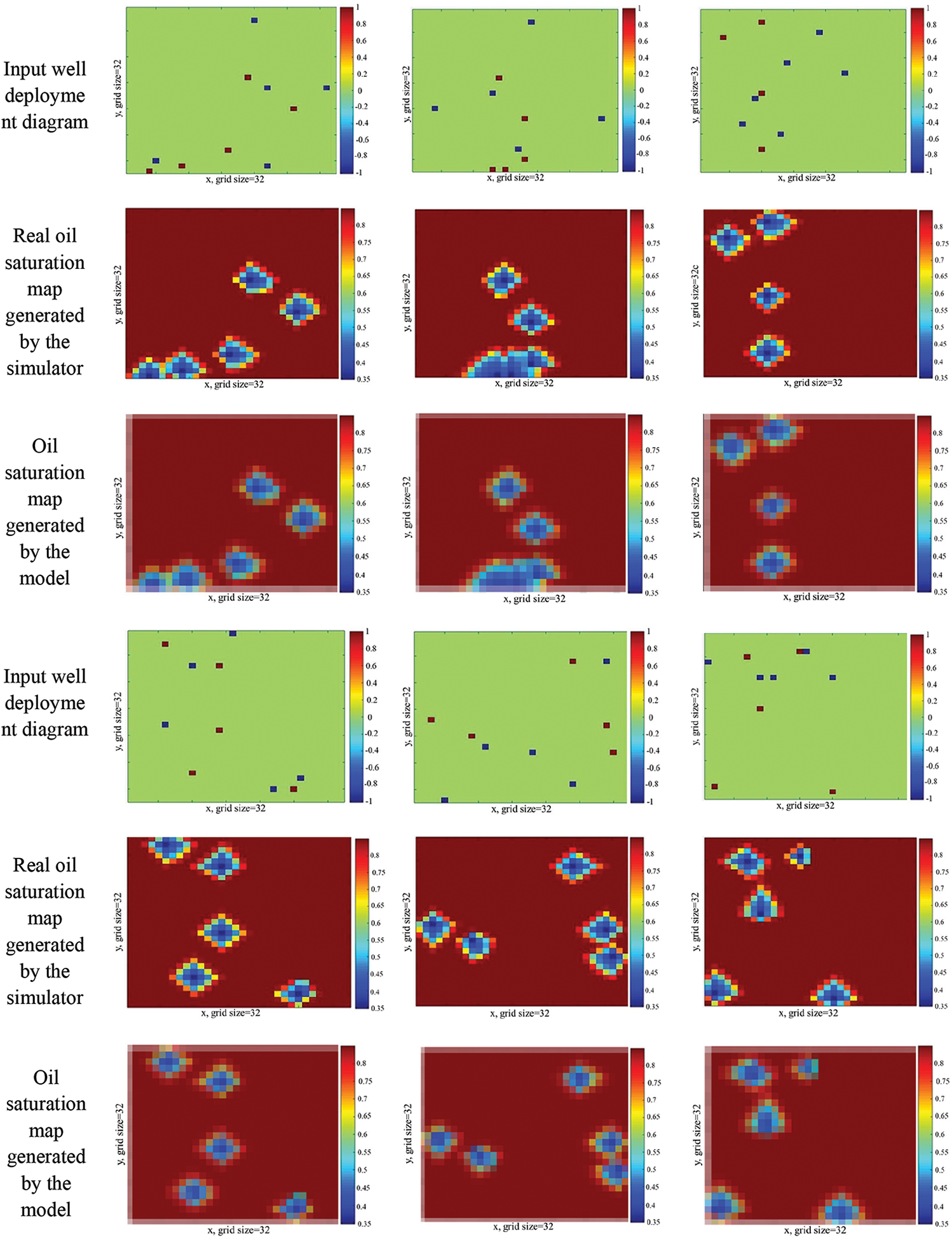
Figure 9: Comparison of oil saturation at 300 days

4  Conclusion

DC-GAN is a model of deep learning and has great advantages in extracting image features and high-dimensional mapping. Based on the DC-GAN framework, the convolution layer and deconvolution layer are used to extract the feature of well location deployment images, and the oil saturation images are output. The real oil saturation map and the oil saturation map generated by the DC-GAN model are distinguished. Then, the model is continuously trained by the discriminant results, and an efficient proxy model for the dynamic mapping of well location deployment to oil saturation distribution is established. The actual example shows that the model can predict the distribution of oil saturation in the case of water flooding with high efficiency and high accuracy. By comparing the cosine similarity between the model results in different time points and the oil saturation images from the numerical simulator, good image similarity is found, which also verifies the good performances of the DC-GAN based proxy model. In addition, the work done in this paper may provide a reference for the application of DC-GAN to more reservoir engineering fields.

Funding Statement: The authors thank the supports from the National Natural Science Foundation of China (No. 52104017), the Open Foundation of Cooperative Innovation Center of Unconventional Oil and Gas (Ministry of Education & Hubei Province) (No. UOG2022-14), and the open fund of the State Center for Research and Development of Oil Shale Exploitation (33550000-21-ZC0611-0008).

Conflicts of Interest: The authors declare that they have no conflicts of interest to report regarding the present study.

References

 1.  Zhou, Z., Song, H., Meng, L., Yu, X., Yu, X. (2002). Numerical simulation of well-pattern optimization in low permeability fractured reservoir—An example of Liang jing oilfield. Xinjiang Petroleum Geology, 23(3), 228–230. DOI 10.3969/j.issn.1001-3873.2002.03.015. [Google Scholar] [CrossRef]

 2.  Cao, R., Cheng, L., Xue, Y., Zhou, T., Xv, J. (2007). Well pattern optimization adjustment for low permeability oilfield. Southwest Petroleum University, (4), 67–69. DOI 10.3863/j.issn.1674-5086.2007.04.016. [Google Scholar] [CrossRef]

 3.  Zhao, J., He, Y., Fan, J., Li, S., Wang, S. (2014). Optimization technology for horizontal well pattern in ultra-low permeable tight reservoirs. Southwest Petroleum University (Science & Technology Edition), 36(2), 91–98. DOI 10.11885/j.issn.1674-5086.2012.05.03.01. [Google Scholar] [CrossRef]

 4.  Zhang, C., Jiang, H. (2014). Optimization method of hydraulically fractured horizontal well pattern in low permeability reservoirs. Fault-Block Oil & Gas Field, 21(1), 69–73. DOI 10.6056/dkyqt201401017. [Google Scholar] [CrossRef]

 5.  Cai, X., Tang, H., Zhou, K., Lu, L., Yang, B. (2010). Study on well pattern optimization method for fractured horizontal well development in low permeability thin interbed reservoir. Special Oil and Gas Reservoirs, 17(4), 72–74, 124. DOI 10.3969/j.issn.1006-6535.2010.04.021. [Google Scholar] [CrossRef]

 6.  Zhao, C., Li, P., Guo, Z., Liu, Q. (2008). Study on the productivity calculation method of staggered well pattern in low permeability anisotropic reservoir. Special Oil and Gas Reservoir, 15(6), 67–70, 98–99. DOI 10.3969/j.issn.1006-6535.2008.06.019. [Google Scholar] [CrossRef]

 7.  Zhang, K., Li, Y., Yao, J., Liu, J., Yan, X. (2010). Theoretical research on production optimization of oil reservoirs. Acta Petrolei Sinica, 31(1), 78–83. [Google Scholar]

 8.  Yao, J., Wei, S., Zhang, K., Jiang, J. (2012). Constrained reservoir production optimization. Journal of the China University of Petroleum, 36(2), 125–129, 135. DOI 10.3969/j.issn.1673-5005.2012.02.021. [Google Scholar] [CrossRef]

 9.  Zhao, H. (2011). Theoretical research on reservoir closed-loop production optimization. Journal of China University of Petroleum. DOI 10.7666/d.y1877014. [Google Scholar] [CrossRef]

10. Ling, Z., Wang, L., Hu, Y., Li, B. (2008). Flood pattern optimization of horizontal good injection. Petroleum Exploration and Development, 1, 85–91. DOI 10.3321/j.issn:1000-0747.2008.01.015. [Google Scholar] [CrossRef]

11. Ling, Z., Hu, Y., Li, B., Wang, L. (2007). Optimization of horizontal injection and production pattern. Petroleum Exploration and Development, 65–72. DOI 10.3321/j.issn:1000-0747.2007.01.013. [Google Scholar] [CrossRef]

12. Chen, Y. (2013). The study and application of smart well pattern optimization. Qingdao, China: China University of Petroleum (East China). [Google Scholar]

13. Fahad, I. S., Khan, M., Yusuf, R., Thakur, K. (2016). Successful application of a mechanistic coupled well-bore-reservoir dynamic simulation model to history match and plan cleanup operation of long horizontal wells. Abu Dhabi International Petroleum Exhibition and Conference. Abu Dhabi, UAE: Society of Petroleum Engineer. [Google Scholar]

14. Fahad, I. S., Salem, A. (2021). Smart shale gas production performance analysis using machine learning applications. Petroleum Research. DOI 10.1016/j.ptlrs.2021.06.003. [Google Scholar] [CrossRef]

15. Khan, M. Y., Yusuf, R. (2016). Co-development plan optimization of complex multiple reservoirs for giant offshore middle east oil field. Abu Dhabi International Petroleum Exhibition & Conference, Abu Dhabi, UAE, Society of Petroleum Engineers. [Google Scholar]

16. Syed, F. I., Al, S. S., Khedr, O. (2021). Infill drilling and well placement assessment for a multi-layered heterogeneous reservoir. Journal of Petroleum Exploration and Production, 11(2), 901–910. DOI 10.1007/s13202-020-01067-0. [Google Scholar] [CrossRef]

17. Pan, S., Liang, H., Li, L., Yang, S. C. (2012). Research on dynamic prediction of oil saturation with GA-BP neural network. Computer Technology and Development, 22(12), 4. [Google Scholar]

18. Hou, C. (2019). New well oil production forecast method based on long-term and short-term memory neural network. Petroleum Geology and Recovery Efficiency, 26(3), 105–110. DOI 10.13673/j.cnki.cn37-1359/te.2019.03.014. [Google Scholar] [CrossRef]

19. Ma, L., Li, D., Guo, H. (2015). Application of BP neural network optimized by genetic algorithm in crude oil yield prediction: A case study of BED test area in Daqing Oilfield. Mathematics in Practice and Theory, 45(24), 117–128. [Google Scholar]

20. Yang, T. (2013). Research on prediction model and algorithm of oilfield development index based on artificial neural network. Daqing, China: Northeast Petroleum University. [Google Scholar]

21. Li, C., Tan, M., Zhang, K. (2011). Oil well production prediction based on improved BP neural network. Science and Technology and Engineering, 11(31), 7766–7769. DOI 10.3969/j.issn.1671-1815.2011.31.038. [Google Scholar] [CrossRef]

22. Fan, L., Zhao, M., Yin, C. (2013). Dynamic analysis method of oil field production based on BP neural network. Fault Block Oil and Gas Field, 20(2), 204–206. DOI 10.6056/dkyqt201302017. [Google Scholar] [CrossRef]

23. Yang, Y., Fu, Q., Wan, D. (2017). A prediction model for time series based on deep recurrent neural network. Computer Technology and Development, 27(3), 35–35. DOI 10.3969/j.issn.1673-629X.2017.03.007. [Google Scholar] [CrossRef]

24. Gu, J., Ren, Y., Wang, Y. (2020). Prediction methods of remaining oil plane distribution based on machine learning. Journal of China University of Petroleum (Edition of Natural Science), 44(4), 39–46. DOI 10.3969/j.issn.1673-5005.2020.04.005. [Google Scholar] [CrossRef]

25. Gu, J., Sui, G., Li, Z. (2018). Oil well production prediction based on ARIMA-Kalman filter data mining model. Journal of Shenzhen University (Science and Technology), 35(6), 575–581. DOI 10.3724/SP.J.1249.2018.06575. [Google Scholar] [CrossRef]

26. Gu, J., Zhou, M., Li, Z. (2019). Oil well production forecast with long: short term memory network model based on data mining. Special Oil & Gas Reservoir, 26(2), 77–81, 131. DOI 10.3969/j.issn.1006-6535.2019.02.013. [Google Scholar] [CrossRef]

27. Negash, B. M., Yaw, A. D. (2020). Production prediction of waterflooding reservoir based on artificial neural network. Petroleum Exploration and Development, 47(2), 357–365. [Google Scholar]

28. Rao, X., Zhao, H., Deng, Q. (2020). Artificial-neural-network (ANN) based proxy model for performances forecast and inverse project design of water huff-n-puff technology. Journal of Petroleum Science and Engineering, 195, 107851. DOI 10.1016/j.petrol.2020.107851. [Google Scholar] [CrossRef]

29. Wang, H., Mu, L., Shi, F. (2020). Production prediction at ultra-high water cut stage via recurrent neural network. Petroleum Exploration and Development, 47(5), 1009–1015. DOI 10.1016/S1876-3804(20)60119-7. [Google Scholar] [CrossRef]

30. Li, D., Liu, X., Cha, W., Yang, J. (2020). Automatic well test interpretation based on convolutional neural network for a radial composite reservoir. Petroleum Exploration and Development, 47(3), 583–591. DOI 10.1016/S1876-3804(20)60079-9. [Google Scholar] [CrossRef]

31. Feng, Q., Li, Y., Wang, S. (2020). Predicting gas migration development using deep convolutional generative adversarial network. Journal of China University of Petroleum (Edition of Natural Science), 44(4), 20–27. DOI 10.3969/j.issn.1673-5005.2020.04.003. [Google Scholar] [CrossRef]

32. Sun, W., Durlofsky, L. J. (2017). A new data-space inversion procedure for efficient uncertainty quantification in subsurface flow problems. Mathematical Geosciences, 49(6), 679–715. DOI 10.1007/s11004-016-9672-8. [Google Scholar] [CrossRef]

33. Yu, X., Fu, Z., Ge, C. (2021). A multi-scale generative adversarial network for real-world image denoising. Signal, Image and Video Processing, 1–8. DOI 10.1007/s11760-021-01984-5. [Google Scholar] [CrossRef]

34. Mo, S., Zhu, Y., Zabaras, N. (2019). Deep convolutional encoder-decoder networks for uncertainty quantification of dynamic multiphase flow in heterogeneous media. Water Resources Research, 55(1), 703–728. DOI 10.1029/2018WR023528. [Google Scholar] [CrossRef]

35. Sun, A. Y. (2018). Discovering state-parameter mappings in subsurface models using generative adversarial networks. Geophysical Research Letters, 45(20), 11137–11146. DOI 10.1029/2018GL080404. [Google Scholar] [CrossRef]

36. Liu, S., Yu, M., Li, M. (2019). The research of virtual face based on deep convolutional generative adversarial networks using tensor flow. Physica A: Statistical Mechanics and its Applications, 521(1), 667–680. DOI 10.1016/j.physa.2019.01.036. [Google Scholar] [CrossRef]

37. Guo, Z., Wan, Y., Ye, H. (2019). A data imputation method for multivariate time series based on generative adversarial network. Neurocomputing, 360(7), 185–197. DOI 10.1016/j.neucom.2019.06.007. [Google Scholar] [CrossRef]

38. Gao, F., Yang, Y., Wang, J. (2018). A deep convolutional generative adversarial networks (DCGANs)-based semi-supervised method for object recognition in synthetic aperture radar (SAR) images. Remote Sensing, 10(6), 846. DOI 10.3390/rs10060846. [Google Scholar] [CrossRef]

39. Patricia, L. S. (2017). Colorizing infrared images through a triplet conditional DCGAN architecture. Cham, Switzerland: Springer International Publishing AG. [Google Scholar]

40. Gan, L., Shen, H., Wang, Y., Zhang, Y. (2021). Data augmentation method based on improved deep convolutional generative adversarial networks. Journal of Computer Applications, 41(5), 1305–1313. DOI 10.11772/j.issn.1001-9081.2020071059. [Google Scholar] [CrossRef]

41. Shibo, L. (2019). DA-DCGAN: An effective methodology for DC series Arc fault diagnosis in photovoltaic systems. Piscataway: IEEE. [Google Scholar]

42. Mohammed, A. B. M. (2019). A novel method for traffic sign recognition based on DCGAN and MLP with PILAE algorithm. Piscataway: IEEE. [Google Scholar]

43. Mohammed, A. B. M. (2020). Pseudoinverse learning autoencoder with DCGAN for plant diseases classification. Berlin/Heidelberg, Germany: Springer Science Business Media, LLC, Part of Springer Nature. [Google Scholar]

44. Zhu, Y., Zabaras, N. (2018). Bayesian deep convolutional encoder-decoder networks for surrogate modeling and uncertainty quantification. Journal of Computational Physics, 366(17), 415–447. DOI 10.1016/j.jcp.2018.04.018. [Google Scholar] [CrossRef]

45. Lie, K. A. (2012). Open-source MATLAB implementation of consistent discretization on complex grids. Computational Geosciences, 16(2), 297–322. DOI 10.1007/s10596-011-9244-4. [Google Scholar] [CrossRef]

46. Peng, X., Rao, X., Huang, L., Xu, Y. (2022). A proxy model to predict reservoir dynamic pressure profile of fracture network based on deep convolutional generative adversarial networks (DCGAN). Journal of Petroleum Science and Engineering, 208(2), 109577. DOI 10.1016/j.petrol.2021.109577. [Google Scholar] [CrossRef]

This work is licensed under a Creative Commons Attribution 4.0 International License, which permits unrestricted use, distribution, and reproduction in any medium, provided the original work is properly cited.