Energy Engineering

---

DOI: 10.32604/ee.2022.021154

ARTICLE

Optimal Intelligent Reconfiguration of Distribution Network in the Presence of Distributed Generation and Storage System

Gang Lei1,* and Chunxiang Xu2

1School of Mechatronics & Vehicle Engineering, Zhengzhou University of Technology, Zhengzhou, 450044, China
2Civil Engineering College, Zhengzhou University of Technology, Zhengzhou, 450044, China
*Corresponding Author: Gang Lei. Email: lei_5345@163.com
Received: 30 December 2021; Accepted: 04 March 2022

1  Introduction

The use of small generators for power generation has gradually faded with the construction of big power plants. However, the growth of consumption, economic-geographic limitations of power transmission, the evolution of the power electronic technologies, restructuring of the power industry, and environmental problems have led to the re-consideration and re-use of these generators in the power generation industry. According to the definition, distributed generation (DG) refers to the electric energy generation units with a capacity of less than 10 MW, in which the distribution feeders or customer levels are connected to the grid in the stations [1]. The connection of DG to the distribution grid can have positive or negative effects on the grid’s performance, depending on the capacity and location of the resources [2]. Besides, DG changes the power flux in the distribution grid, resulting in which the main structure of the grid will no longer be optimal for loss reduction in the presence of the DG. Therefore, the grid requires a new reconfiguration to optimize the cost and improve the grid’s reliability [3]. To increase the reliability and reduce the outages of the distribution grid, the grids are commonly designed in a circular form; however, to lower the short-circuit level and coordinate the protection systems, these grids are operated radially, which will result in the increased loss in the grid. Therefore, the DFR is executed through switching management in the distribution grid to reduce the losses, improve reliability, and so on. In the reconfiguration process, the distribution feeders are reconfigured about the status of the switches to achieve different goals. In the reconfiguration process, some constraints, including maintenance of the radial structure of the grid after the reconfiguration, feeding of all loads, care of the voltage of the buses in the specified range, and loading of the lines, must be met [4]. The DFR is a nonlinear and non-convex problem; thus, mathematical methods are not suitable for this purpose due to the limitations of the objective functions and constraints such as discontinuity and differentiability. So far, numerous studies have been conducted on the distribution grid reconfiguration; but most of these studies have not investigated the effect of DG on the operation of the distribution grid in detail. The necessity and benefits of reconfiguration in normal conditions in distribution grids can be studied in terms of the following aspects [5]:

a) Loss reduction: Today, loss reduction in distribution grids is the most critical priority in the design and operation of power grids. In power supply networks, a considerable percentage of the electric energy generated in power plants is wasted in the path from generation to consumption. The losses can occur at all power systems, including generation, transmission, and distribution. Yet, nearly 75% of the losses occur in the distribution system. Recent studies have shown that almost 5%–13% of the total generated power is lost as the line losses in the distribution grid [6]. Several methods have been proposed so far for loss reduction, including capacitor placement, consumption management for peak shaving, replacement of grid conductors, changing the voltage level, load management of transformers, and grid reconfiguration. Among these methods, reconfiguration is the simplest and lowest-cost method for loss reduction. The profit-to-cost ratio of each of the methods mentioned above is presented in Table 1 [7].

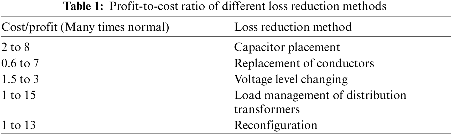
As shown in the above table, the two methods of “load management of distribution transformers” and “reconfiguration” have the highest profit-to-cost ratio.

b) Voltage stability improvement: Due to the high current and high R/X ratio in distribution grids, the voltage drop is considered a severe problem. In recent decades, due to the growing increase in subscribers and the problems occurring in the construction, operation, and repair of the power plant units and transmission network, the power systems have undergone excessive loading. As a result, many power systems and, consequently, distribution grids worldwide have been exposed to a phenomenon known as voltage instability. There are various methods for improving the power grid voltage stability, one of which is grid reconfiguration [8].

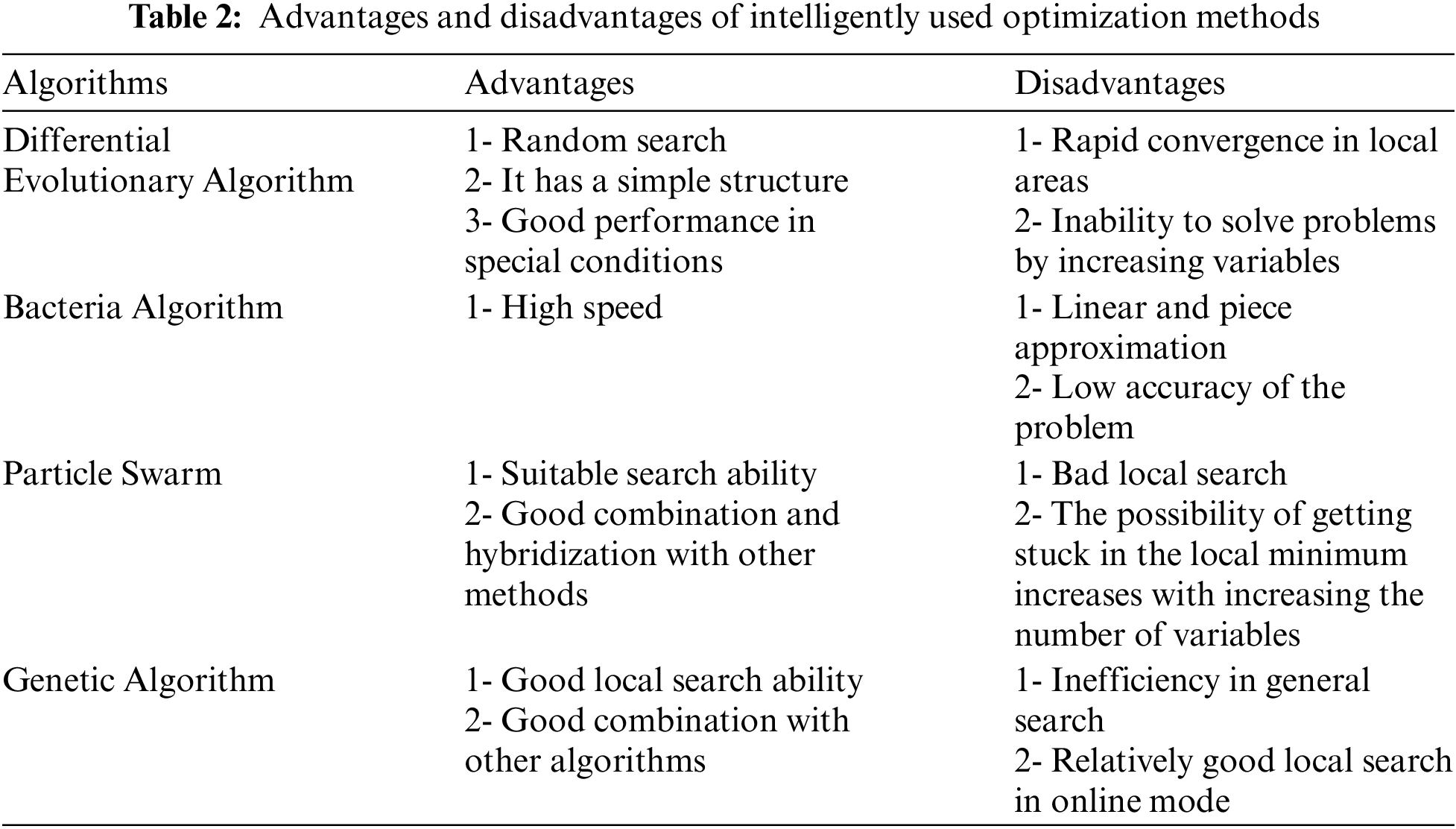
c) Load balance between feeders: The load imbalance in the distribution grid results not only in an unnecessary occupation of the capacity of the grid and equipment but also in increased electric energy loss and, thereby, increased investment cost. When the equipment is added to balance the load, in addition to the significant equipment purchase investment costs, the costs of the equipment repair and maintenance will be increased [9]. There are various methods for load balance, among which the reconfiguration method can establish the load balance between the feeders while maintaining the existing facilities and without adding any equipment. Reconfiguration causes the load flows to be transferred from one feeder to another, yielding the load balance. Since the reconfiguration problem is an optimization problem with several objectives and limitations, two different scenarios have been considered for this purpose. In the first scenario, loss reduction, load balance between feeders, and the number of switching operations are assumed as the objectives. In the second scenario, the objectives include loss reduction, voltage stability improvement, and reduction in switching operations [10]. In most of the studies distribution grid reconfiguration in the presence of DGRs, the resource has been assumed as a negative load in the reconfiguration problem. (PQ model). In the present paper, the PQ and PV models are compared. To model the PV busbars, two compensation technique-based methods are used. In the first method, the reactance sensitivity matrix is used, described in [11]. A disadvantage of this method is that it requires repetitive distribution of loads. Thus, the reconfiguration problem, in which we face several configurations, will be very time-consuming. In the present work, this problem is solved using genetic algorithm (GA) so that the algorithm determines the optimal configuration and the reactive power of the DG simultaneously. In [12], the bacteria foraging algorithm (BFA) was used as a new method for distribution grid reconfiguration. The researchers claimed that this algorithm had a better performance than the GA in implementation, flexibility, and speed of convergence to the optimal solution. Besides, this algorithm can be useful and have higher capabilities to be applied to real systems on a large scale. In [13], a new evolutionary method based on a hybrid PSO-Nelder-Mead algorithm was used to solve the reconfiguration problem. In this method, in order to improve efficiency, the PSO was combined with the developed method. The proposed plan had high precision and speed. The power loss was the objective function in this reference. In addition to the previous limitations, the number of switching operations was added to the optimization problem. In [14], the authors proposed a hybrid SFLA-PSO algorithm for solving the distribution grid reconfiguration problem reduce the losses and improve the voltage stability in the presence of the DGRs. In [15], a hybrid GWO-PSO algorithm was used for solving the problem of dynamic DFR in the presence of DGRs in order to reduce the losses and operation costs. Also, an improved GSA algorithm was proposed for solving the DFR problem in the presence of the DGRs, aiming to improve the transient stability index. In [16], an improved hybrid SFLA-PSO algorithm was proposed for solving the problem of dynamic DFR and capacitor switching in the presence of the DGRs and ESSs [17]. In [18], the ANO algorithm was used for solving the problem of dynamic DFR and switching of capacitor banks in the presence of DGRs with the aim of reducing the losses. Also, an improved hybrid SFLA-PSO algorithm was proposed for solving the problem of reconfiguration and capacitor switching in a dynamic framework to minimize the grid operation costs. Although these algorithms are good methods for optimization and design problems. However, if the number of optimization parameters is higher, their efficiency decreases and the computation time increases. This makes them impossible to use in timely applications and large-scale systems such as real power systems. Table 2 shows a comparison of the different methods.

In the above-mentioned papers and in most of the studies on the reconfiguration problem, the effect of DG on the distribution system's operation has not been investigated in detail. However, in the present paper, the DFR problem is investigated considering different models of DG and ESS in terms of loss reduction and voltage stability. Also, a developed PSO algorithm with self-adaptive time-varying particles is used to solve the reconfiguration problem. Regarding the alternative behavior of the DGRs, most of the references in this field have not taken the uncertainty of the power of these resources into consideration. Accordingly, the features of the model presented in this study are as follows:

- Proposed an optimal design for energy management in the presence of the DGRs with energy storage units;

- Consider an appropriate level of reliability and grid security considering the uncertainty in the output power of the DGRs;

- An improved PSO algorithm is presented in this work for dealing with the complexities of the optimization problem;

- The non-distributed energy, energy losses, and voltage stability index are defined as the objective functions of the problem.

The rest of this paper is organized as follows: Section 2 provides the problem formulation. In Section 3, the developed algorithm is proposed. Section 4 presents the results of simulation and numerical analysis on the 33-bus system. Finally, the simulation results are provided in Section 5.

2  Problem Modeling

In this section, each of the objective functions will be modeled. Then, each of them will be normalized to form a multi-objective function inspired by the fuzzy sets. Afterward, a membership function will be assigned to each objective, so that the membership function will indicate the satisfactoriness level of the objective. Since each function takes a value between zero and a unit (not merely zero and one) in the fuzzy logic, the above multi-objective optimization problem will have higher flexibility.

2.1 Membership Function for Loss Reduction

The loss value can be obtained using the following equation:

PLOSS=∑k=1l|Ik|2Rk(1)

where PLOSS is the total power loss, Ik is the current flowing in branch k, Rk is the resistance of branch k, and 1 is the number of feeders. The power loss ratio is defined as follows:

PLt=PLOSS,tPLOSS,0(2)

where PLOSS,t is the total power loss for the ith design of reconfiguration and PLOSS,0 is the total power loss before the reconfiguration.

The membership function for loss reduction is illustrated in Fig. 1.

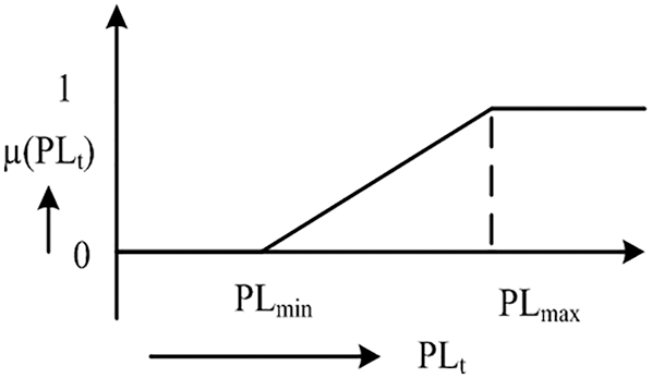
Figure 1: Membership function for loss reduction

Regarding the above figure, μ(PLt) is obtained from the following equation:

μ(PLt)={(PLt−PLmin)(PLmax−PLmin),PLmin<PLt<PLmax0,PLt≥PLmin1,PLt≥PLmax(3)

2.2 Membership Function for Load Balance

The load balance index is defined as follows:

Bt=∑k∈B(|Ik,t|Ik max)2(4)

where Bt is the load balance index for the ith design of reconfiguration, B is the set of branches forming the ring in the grid, Ik,t is the current of the kth branch for the ith design of reconfiguration, and Ikmax is the maximum current that branch k can tolerate. The load balance index defined in Eq. (4) is normalized as follows:

LBt=BtB0(5)

where LBt is the normalized LBI for the ith design of reconfiguration and B0 is the LBI before the reconfiguration. The membership function of the load balance is depicted in Fig. 2.

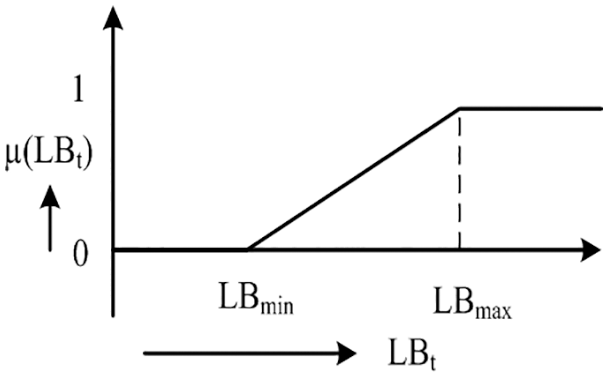
Figure 2: Membership function for load balance

According to Fig. 2, μ(LBt) is obtained from the following equation:

μ(LBt)={(LBt−LBmin)(LBmax−LBmin),LBmin<LBt<LBmax0,LBt≥LBmin1,LBt≥LBmax(6)

2.3 Membership Function for the Number of Switching Operations

Fig. 3 illustrates the membership function for the number of switching operations.

Figure 3: Membership function for the number of switching operations

Regarding Fig. 3, μ(SWt) is obtained from the following equation:

μ(SWt)={(SWt−SWmin)(SWmax−SWmin),SWmin<SWt<SWmax0,SWt≥SWmin1,SWt≥SWmax(7)

where SWt is the number of switching operations for the ith design of reconfiguration.

2.4 Objective Function

In this section, we will combine the three above-mentioned objective functions by weighted factors. For each of these objectives, a weighted factor is considered. Then, the three objective functions normalized using the fuzzy sets theory are modeled as a multi-purpose objective function, as follows:

F=∑X=13WX.fX(8)

where fX for X=1,2,3 is the objective function of loss reduction, reduction of load balance defined in Eq. (4), and reduction of the number of switching operations, respectively. Also, constants W1 and W2, respectively, assign the corresponding weight to each of these objective functions. Regarding the conditions of the system and the intended objective functions, the solution of the multi-objective problem can be directed toward the given criteria by changing and adjusting the weighted coefficients. Besides these multi-purpose objective functions, the following constraints must be met [19]:

1) Load distribution equations: The sum of the powers flowing in the branches connected to the ith bus is equal to the load demand in the ith bus.

2) Voltage limitation of the buses: The voltage of the buses must remain in the permitted range.

Vmin≤Vi≤Vmax(9)

3) Current limitation of the feeders: The current flowing in the feeders cannot exceed the permitted level due to thermal limitations.

|Ik|≤Ikmax(10)

4) Limitation of radial structure of the grid: The grid must keep its radial structure.

5) Limitation of load non-discontinuity: The grid must be reconfigured in such a way that no load is separated from the grid and all the buses must have energy.

2.5 Radial Structure Recognition Algorithm

To recognize the radial structure, the bust incidence matrix is used. The procedure of the algorithm is as follows [20]:

1) Form the bus incidence matrix A^. The dimension of this matrix is (1×n), so that 1 is the number of branches of the grid and n is the number of the buses. Also, aij is assumed as the entry of the ith row and jth column as follows:

If the branch between bus i and bus j exits bus I, then, aij=1; if it enters bus I, then, aij=−1. But, if there is no branch between these two buses, then, it is assumed that aij=0.

2) After forming A^, eliminate the column corresponding to the base bus from matrix A^. The newly obtained matrix is indicated by A. The dimension of matrix A will be (B×N), so that B is the number of the branches of the grid and N is the number of the buses of the grid without considering the reference bus.

3) If the primary grid has no ring, then matrix A obtained from the previous step will be a square matrix. If matrix A is a square matrix, then two states will occur: (det(A)=1ordet(A)=−1).

1- If determinant of A is equal to 1 or –1 (det(A)=1ordet(A)=−1), then, the structure of the grid will be radial.

2- If determinant of A is equal to 0, then, the grid will not be radial and a group of the loads go out of service.

2.6 Introduction of the Voltage Stability Index

In the previous section, the objectives of the removal of losses and reduction of the number of switching operations were introduced; thus, there is no need to introduce them again. In this section, the voltage stability index of the buses is defined. In a distribution grid, due to the high value of the current and R/X ratio, the problem of voltage drop is taken into consideration seriously. With an increase in the load demand in the distribution grid, the occurrence probability of the voltage collapse is intensified. Therefore, it is necessary to identify and determine the buses that are exposed to voltage fluctuations more than others [21]. Using the sensitivity analysis technique, a stability index is defined for each bus. This index identifies the most sensitive bus that is exposed to voltage collapse. Also, it can be obtained from the quadratic equations used in the load distribution algorithms of the distribution grids to calculate the voltage. This equation is written as follows:

Vr4+2Vr2(P.R+Q.X)−Vs2Vr2+(P2+Q2)|Z|2=0(11)

where Vs and Vr indicate the voltage domain in the sender (s) and receiver (r) buses, respectively. Also, Z is the impedance of the connector line between the above two buses, and P and Q are the active and reactive powers transmitted from bus s to bus r, respectively. Eqs. (12)–(15) have four roots. The maximum positive value of the roots is obtained as follows:

Vr=0.707[b+(b2−4c)1/2]1/2(12)

where:

b=Vs2−2PR−2QX(13)

and

C=(P2_+Q2)(R2+X2)(14)

Regarding Eq. (12), the real value of the voltage domain in the receiver bus r will exist under the following conditions:

b2−4c≥0(15)

By setting Eq. (15) equal to zero, the critical point of the loading of the grid will be obtained. Therefore, the equation indicating the voltage stability index in receiver bus r is obtained as follows:

VSI(r)=Vs4−4(P.X−Q.R)2−4Vs2(P.R+Q.X)(16)

The bus with the smallest VSI index will be recognized as the bus with the highest sensitivity to voltage collapse (critical bus). This index is equal to 1 in the case of no load and equal to zero in the case of voltage collapse.

2.7 Modeling the Electric Energy Storage System (Battery)

To appropriately model and utilize the battery, the two charging and discharging modes were modeled as follows. One of the most critical battery-related parameters is the SOC (state of charge) of the battery, the value of which in the fully-charged state is equal to 1 and, in the fully-discharged state, is equal to zero. This variable is obtained every hour from the state of the previous hour and the battery power at that hour. The SOC indicates the current state of the charge compared to the total capacity of the battery and represents the battery's charging value or, in other words, the amount of energy remained in the battery. It is expressed as the percentage ranging from zero to 100 [22]. In the present paper, this parameter is presented at every hour of the day.

SOCt=EtCAPbar×100(17)

where Et is the amount of power charged at hour t and CAPbar is the nominal capacity of the battery. Then, instead of SOC, variables xtBp and xtBn indicate the charging and discharging states, respectively.

It is evident that the battery cannot be in the charging and discharging states at the same time. This limitation is modeled by the following equation. In this equation, variables xtBnandxtBp indicate the charging and discharging states of the storage, respectively. For example, if the value of xtBp is equal to 1, it means that the battery is in the charging state and, thus, the value of xtBn will be equal to zero:

xtBp+xtBn≤1(18)

It is necessary to say that a battery cannot be completely discharged for the reason it will be damaged seriously and irreversibly, and will become unusable. Therefore, a portion of the nominal capacity is assumed as the inactive capacity. The below equation guarantees the discharging value in each period is less than the amount of the available charge of the battery in period t:

xtBn<xtBp(19)

The energy stored in the battery at each moment must be between its minimum and maximum permitted values. The battery's capacity constraint (limitation) is expressed by the following inequality, where Emin.B and Emax.B indicate the minimum and maximum capacity of the system, respectively, and EOB represents the initial capacity:

Emin.B≤EOB+Et≤Emax.B(20)

2.8 Radial Load Distribution Algorithm

To study the static behavior of the distribution systems, calculating the load distribution is one of the critical calculations. Importing the DG into the calculation makes the high-precision calculations more complicated. In the presence of DG, the commonly used methods of load distribution in distribution systems are not much efficient. Thus, it is necessary to modify these methods to import the DG that is commonly modeled in the distribution grids PQ or PV buses. Generally, the common methods of load distribution are divided into three groups: The Newton-Raphson technique-based methods, the Zbus Gauss technique-based methods, and dynamic (backward-forward sweep) methods [23]. However, due to some special features of the distribution grid such as radial structure and high R/X ratio, the common load distribution methods in grids, including Gauss-Seidel and Newton-Raphson methods, are not suitable for distribution grids. One of the suitable methods for load distribution in distribution grids is the forward-backward sweep method. The steps of the forward-backward sweep load distribution algorithm are as follows:

1) Backward sweep: By starting from the final buses and moving toward the base bus, the power of the branches is calculated.

2) Forward sweep: By starting from the branch connected to the base bus and moving toward the final branches, the currents are calculated in the sender bus of branch i and the voltages are calculated in the receiver bus of branch j.

3) Calculation of voltage inconsistency: Once the two above steps are done at each repetition, the voltage inconsistency is calculated for all the buses.

4) If the voltage deviation of the buses is more than the convergence criterion, Steps 1 and 2 are repeated to meet the convergence.

In the present paper, the load distribution algorithm is used based on the grid topology. In this method, to execute the backward-forward sweep, first, a BIBC (bus injection to branch current) matrix is formed. The procedure of forming this matrix is as follows. For example, branch currents B1, B3, and B5 are expressed as shown below:

B5=I6

B3=I4+I5

B1=I2+I3+I4+I5+I6(21)

The matrix form of the above equation is as follows:

[B1B2B3B4B5]=[1111101111001100001000001][I2I3I4I5I6](22)

The matrix Eq. (22) is expressed as follows:

[B]=[BIBC][I](23)

By investigating the above matrix equation, the formation algorithm of the BIBC matric is obtained as follows:

1) For a distribution grid with m branches and n buses, the dimension of the BIBC matrix will be (m×n−1).

2) If branch Bk is located between buses i and j, copy the column of the ith bus of the BIBC matrix in the column of the jth bus and put 1 in the kth row and jth column.

3) Continue Step 2 until all lines of the BIBC matrix are covered.

2.9 First Method of Handling DG in the Load Distribution Program

In this method, first, in each PV busbar, the constants are determined for the resource (real output power P and voltage domain V). Then, in the load distribution algorithm, this busbar is assumed as a PQ busbar. When, the load distribution is converged, the following steps must be done [23]:

1) The voltage difference of the PV busbar from the determined value is calculated.

ΔVi=|Vspi−Vcali|≤ε

i=1,2,…,nPV(24)

where ΔVi is the voltage inconsistency in the ith node, nPV is the number of the PV buses, Vspi is the determined value of the voltage domain in the ith busbar, and Vcali is the calculated value of voltage domain in the ith busbar.

2) If the voltage inconsistency is in the determined range, the voltage of the PV bus will converge to the determined value; otherwise, by compensating for the reactive power generated by the DGR, the voltage will be maintained at the determined value in the intended busbar. By ignoring the voltage variations that occur with the changes in the active power, the amount of reactive power required for compensation can be calculated by the following equation:

X.ΔQ=ΔV(25)

where X is the reactance sensitivity matrix of the PV node and its size is (npv−unconverged×npv−unconverged), so that npv−unconverged×1 is the number of the PV buses, the voltage of which has not converged to the determined value. This matrix is obtained as follows.

Diagonal elements of X: is the sum of reactance values of the branches between each unconverged PV bus and the base bus.

Non-diagonal elements of X: are the sum of reactance values of the common branches between two unconverged PV nodes and the base bus. Matrix X is changed during the reconfiguration of the grid.

ΔQ: Vector of the injected reactive power

ΔV: Vector of the voltage inconsistency of the PV buses

The size of both vectors is equal to npv−unconverged×1.

If ΔV>0, the DG resource will generate reactive power to maintain the voltage at the determined value. But if ΔV<0, the resource will absorb reactive power in order to keep the voltage constant at the determined value. Therefore:

Qnewcali=Qoldi±|ΔQi|(26)

where i=1:n, Qnewcali is the new value of the injected reactive power of the resource of the ith busbar and Qoldcali is the calculated value of the generated reactive power of the resource of the ith busbar in the previous repetition.

3) After calculating ΔQ, the generated reactive power of the resource must be controlled through the following equation:

QGmini≤Qnewcali≤QGmaxi(27)

where QGmini and QGmaxi are the lower and upper limits of the generated reactive power of the DG resource. If Eq. (27) is not met, then, the generated reactive power of the resource is set at a value violated by Qnewcali. Now, the backward-forward sweep load distribution problem and the above steps are repeated. This procedure is continued until the voltage of all PV buses converge to the determined value.

3  Developed PSO Algorithm

The PSO algorithm, is very simple to execute and it can obtain the global optimal solution by its high efficiency. However, due to the lack of sufficient search space, the PSO algorithm has a phenomenon that can be easily set in the local optimal state. Although increasing the particle size can improve this feature, it can increase the complexity of the algorithm and fail to solve the fundamental problem [24]. Therefore, the present paper combines the adaptable weight and irregular series. Hence, in this section, the adaptive chaotic particle swarm optimization (ACPSO) algorithm will be introduced.

3.1 PSO

In PSO algorithm, each particle calculates its appropriateness with regard to its position. In each repetition, the updated process, speed, and position of the particle are shown:

vik+1=w.vik+c1.r1.(pbesti−xik)+c2.r2.(gbest−xik)(28)

xik+1=xik+vik(29)

3.2 Adaptive Weight

Adaptive weight mostly balances the local and global search. This approach can change constant w, so that it is reduced adaptively with reduction in the number of repetitions, as described in Eq. (30).

vik+1={[wmin−(wmax−wmin).(fik−pbesti)pbestavg−pbesti].vik+c1.r1.(pbesti−xik)+c2.r2.(gbest−xik),fik≤pbestavgwmax.vik+c1.r1.(pbesti−xik)+c2.r2.(gbest−xik),fik>pbestavg(30)

3.3 Chaotic Search

The main idea of the chaotic search is the repetitive production of chaotic sequences through a certain format. The algorithm must assume the repetitive process as stationary. In other words, the optimal value of the individuals does not change considerably with increasing the particles by more than five times. Eq. (31) requires being quintupled. If Eq. (31) is correct for five times, then, the chaotic search will be needed.

(fik−pbesti)/fik<10−3(31)

In the case of recession, a d-dimensional vector is created randomly with a value between [0,1],Y0=[y0,1,y0,2,…,y0,d]T and Y0∈[0,1]. There is quantitative difference between the elements. With an initial value of Y0, the repetition of the chaos starts with regard to Eq. (32) and, thus, the repetitive sequence of Yn is obtained.

Yn=Yn−1.(1−Yn−1)T(32)

where n=1,…,Nmax.

Then, turbulent solution Yn is searched in the vicinity of the recession solution by Eq. (33). In other words, the position of the particle in region Rd is searched again as the radius with stationary particle as the center.

Y´n=xik+Rd.(2Yn−1)T(33)

Thus, Y´n∈[xik−Rd,xik+Rd]. The value of the objective function f(Y´n) is calculated in the chaotic repetitive process. If f(Y´n) be superior than the local optimal solution of PSO, the major location and local solution of the particle are returned with f(Y´n) andY´n. Moreover, the speed of the particle is updated through Eq. (34).

vik=Y´n−xik||Y´n−xik||(34)

However, the feature of the PSO is that the fitness function is changed in the previous step and a bit in the next step. This means the solution process imports a chaotic search into the next step. Thus, regarding the experience of the solution, another chaotic search will not be done in this paper when the value of the particle is less than 105.

3.4 Steps of ACPSO

Steps of the ACPSO algorithm for solving the MG optimization model are as follows:

Step-1: Running. First, set the dimension of particle d and size of particle n. Then, regarding the domain of the independent variables, n groups of the solutions will be produced randomly in the domain and n groups of the vectors will be produced randomly in the [0,1] interval as the initial speed of the particles.

Step-2: Find the best pbesti and the best gbest close to the global solution. Calculate the value of the objective function fik for each particle. Consider the minimum value of each particle in each repetition process as the optimal individual value, i.e., pbesti=mink{fik}.

Consider the minimum of all optimal individual value of the particles as the optimal value close to the global solution, i.e., gbest=min{pbesti}.

Step-3: Calculate the value of w. Update the speed and position of the particles according to Eqs. (28) and (29). Find the new vik and xik. Calculate the consistency between the objective functions. Regarding Eq. (30), determine whether it is trapped in a local optima or not. Step 4 is done when the solution is in the local optima; otherwise, Step 5 will be done. Moreover, if the sum of all particles is less than 105, the chaotic search will not be done.

Step-4: Chaotic search

Step 4-1: compute the chaotic answer of each repetition based on Eq. (33).

Step 4-2: compute the chaotic function of f(Y´j). Consider the least amount of f(Y´j) as f∗.

Step 4-3: If f∗ is less than the optima close to the global in Step 2, then, consider f∗ as the general optima. Use Yj´ as the particle's position and update the particle's swarm according to Eq. (34). Then, do Step 5. If the highest number of the chaotic is satisfy, Step 4 will be done; or else, go back to step (4–2) for the next generation.

Step-5: Update the speed and location.

Step-6: Decide whether the process should be finished or not. If the accuracy is according to the needs or the number of repetitions, the current optimal solution will be the output. This procedure is shown in the Fig. 4.

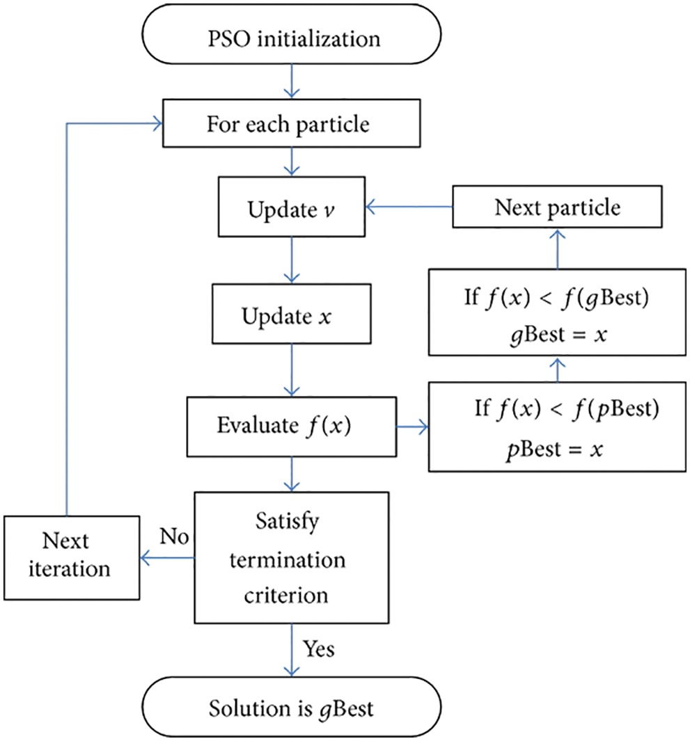
Figure 4: Flowchart of proposed PSO

3.5 Solving the Optimization Problem by the Given Algorithm

Since the proposed model of distribution grid reconfiguration is a nonlinear problem with binary variables, the proposed algorithm is a suitable method for finding the optimal configuration with the assumed objective functions. In this algorithm, first, the switching status of the grid is encoded as binary strings. Then, regarding the objective function, a fitness function is assigned to each string. The proposed fitness function is assumed as follows:

Ffitness=11+∑X=13WX.fX+∑y∈SCKi.Bi(35)

where ∑X=13WX.fX is the weighted set of objective functions and indicates the final multi-purpose objective function. Ffitness is the fitness function. The governing constraints of the problem are taken into account as a penalty function, ∑y∈SCKi.Bi, in the fitness function, so that Ki is the penalty coefficient corresponding to the ith constraint, Bi is the degree of violation of the corresponding constraint, and SC is the set of problem constraints.

4  Simulation Results

4.1 Studied System

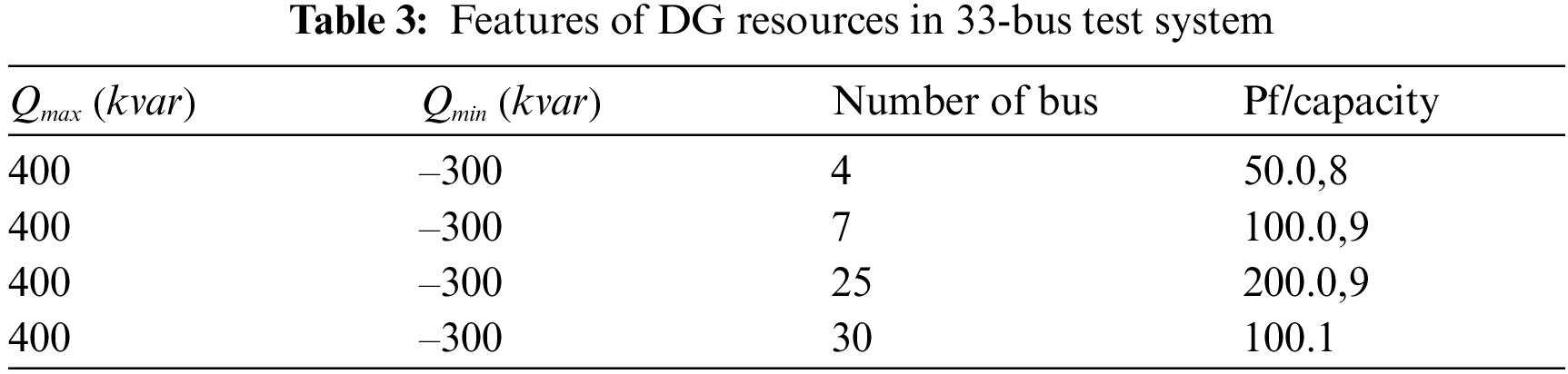
The test system studied in this section is a standard 33-bus distribution grid. This grid is composed of five tie switches and 32 sectionalizing switches. The maximum current that a feeder can tolerate is assumed equal to 200 A in all the branches. The data related to this grid are provided in the appendix. In this grid, four DG resources are installed in buses 25, 7, 4, and 30. The capacity and location of the installed DG resources as well as the range of the generated reactive power of these resources are presented in Table 3.

4.2 First Scenario

This simulation scenario includes three objectives, namely loss reduction, load balance between feeders, and reduction of the number of switching operations. In this scenario, the following five states are investigated:

1) Initial system without reconfigurations.

2) The system is reconfigured in such a way that the losses are reduced.

3) The system is reconfigured in such a way that the load balance index is reduced.

4) The system is reconfigured as in state 2 provided that the number of switching operations does not exceed four operations.

5) The system is reconfigured using the algorithm described in the previous chapter and considering the compromise between the thee above-mentioned objectives.

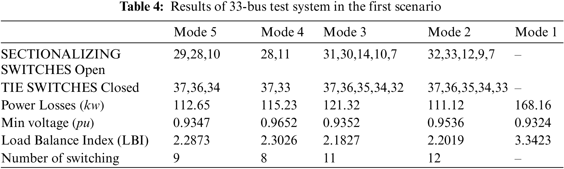
The numerical results for the above-mentioned five states are presented in Table 4. According to the table, state 1 exhibits high power loss and load balance index. Regardless of the DG units, the loss of the system is equal to 202.50 kw. But, in state 1 in the presence of the DGRs, the loss is reduced to 168.16 k, indicating that the DG units usually, but not necessarily, play an important role in the reduction of the losses. Moreover, the minimum voltage of the grid in this state is improved from 0.9024 to 0.9324 on a per-unit system. Besides, the load balance index is reduced from 4.0971 to 3.3423 in state 1, indicating that the DGRs are effective in balancing the load between the feeders. As expected, the system's loss in state 2, the load balance index in state 3, and the number of switching operations in state 4 are minimized. In state 5, by establishing a compromise between the above-mentioned objectives, a multi-purpose objective function is optimized by adjusting the weighted factors, so that W1 is the weighted factor of losses, W2 is the weighted factor of the number of witching operations, and W3 is the weighted factor of load balance. A compromise means that, for example, the loss in state 5 is more than that in state 2. But, state 5 requires only switching operations, instead of 10 operations. Although the load balance between the feeders and branches in state 3 is better than that in state 5, the power loss and switching operations in state 3 are more than that in state 5. Comparing states 4 and 5 shows that although the number of switching operations in state 5 is more than state 4, the power loss is reduced by 1.3 kw. Moreover, the comparison of the load balance indices shows that the loading status of the feeders and branches in state 5 is more balanced than state 4.

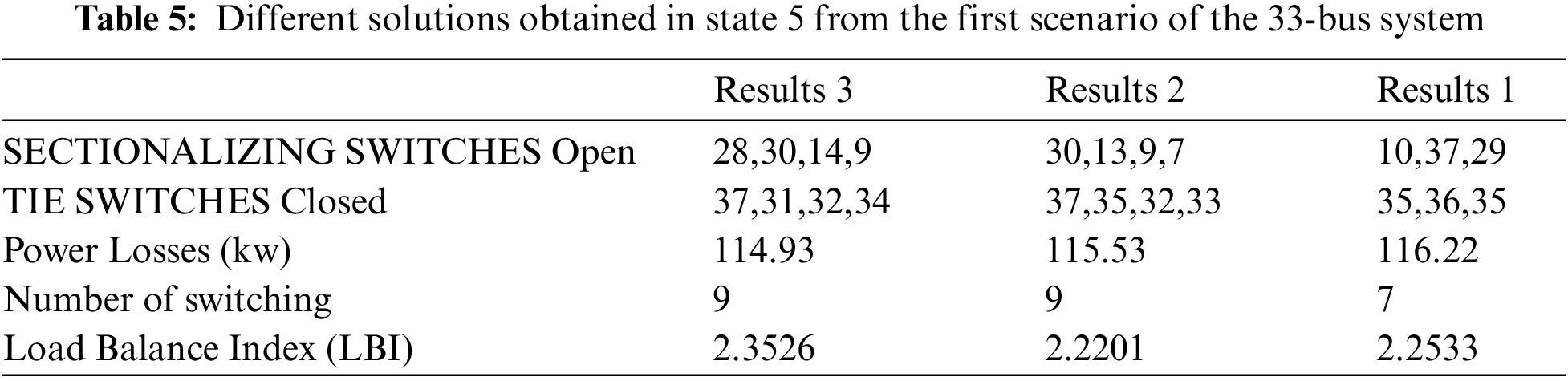
Indeed, by changing and adjusting the weighted factors (depending on the designer’s opinion), other solutions can be also obtained for state 5. For example, some of these solutions in state 5 are presented in Table 5.

To show the convergence of the proposed algorithm, the graph of the losses obtained in state 2 by elite strings in each generation is depicted in Fig. 5.

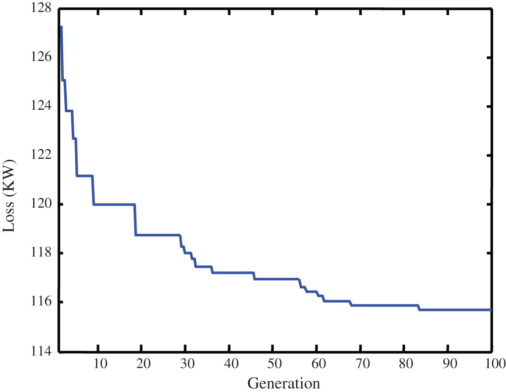
Figure 5: Losses obtained by elite strings in each generation in state 2 from the first scenario of the 33-bus system

The voltage profile of states 1, 2, and 3 and that of states 4 and 5 are depicted in Figs. 6 and 7, respectively.

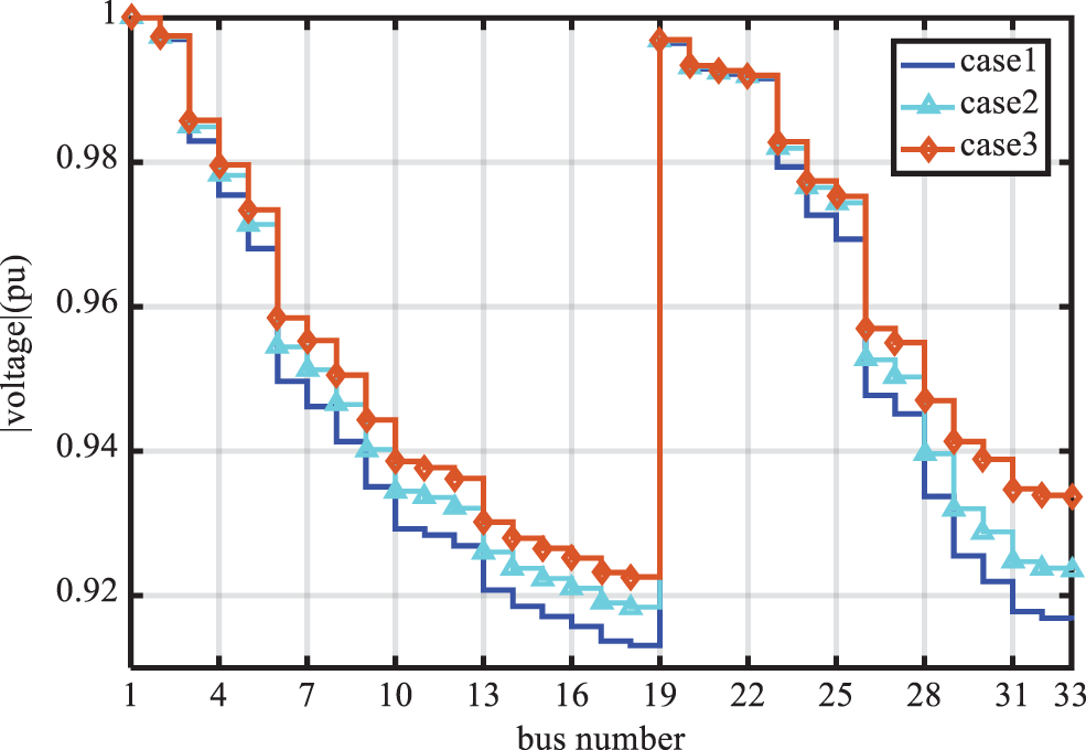
Figure 6: Voltage profile of the buses in states 1, 2, and 3 from the first scenario of the 33-bus system

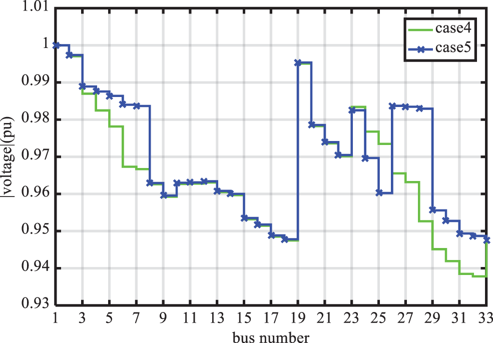
Figure 7: Voltage profile of the buses in states 4 and 5 from the first scenario of the 33-bus system

According to the above figures, in each of states 2 to 5, in which the reconfiguration is performed, the voltage profile status of the buses is improved compared to state 1. In this regard, the best result in terms of the improvement of the minimum voltage is obtained in states 2 and 5. However, even in these states, the voltage of some of the buses exceeds the permitted level.

The current profile of different states is depicted in Figs. 8 and 9. As expected, in states 2 and 3, the current in most of the feeders and branches is reduced compared to state 1. Although the average current of the branches in state 2 is less than that in state 3, the load balance index (i.e., the sum of square of the current of each branch relative to the maximum current that a branch can tolerate) in state 3 exhibits further reduction than state 2.

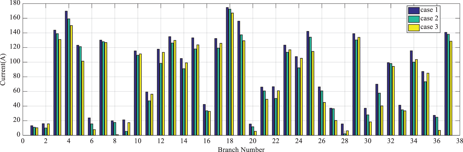
Figure 8: Current of branches in states 1, 2, and 3 from the first scenario of the 33-bus system

In Fig. 9, the current of each branch in state 4 is compared with that in state 5. The average current of the branches in state 4 is less than that in state 5, but since those branches that have lower current in state 5 than state 4 commonly have higher resistance, they will cause more loss reduction than state 4. Therefore, the active losses of the branches in state 5 will be less than that in state 4.

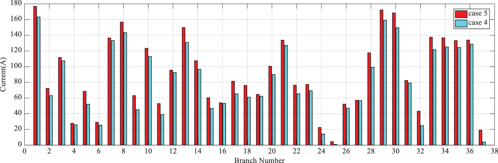
Figure 9: Current of branches in states 4 and 5 from the first scenario of the 33-bus system

The active and reactive losses of the branches in different states are depicted in Figs. 10–13. According to Fig. 10, in each of states 2 and 3, the total active loss of the branches is reduced compared to state 1. Also, state 2 exhibits maximum reduction.

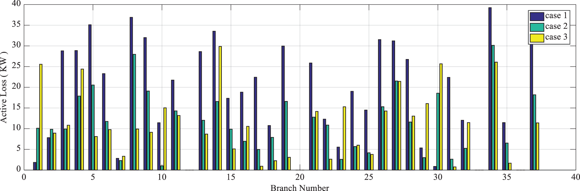
Figure 10: Active loss of branches in states 1, 2, and 3 from the first scenario of the 33-bus system

According to Fig. 11, the total active loss of the branches in state 5 is less than that in state 4. However, as mentioned earlier, the average current in state 4 is less than that in state 5.

According to Figs. 12 and 13, it is observed that in states 2 to 5, in which the reconfiguration is performed, the total reactive loss of the branches is reduced compared to state 1. Also, the reactive loss of the grid in states 4 and 5 exhibits more reduction than other states. Therefore, these states (i.e., states 4 and 5), respectively, will have the best status in terms of the improvement of the average voltage of the grid. As mentioned earlier, states 2 and 5 have the best status in terms of the improvement of the minimum voltage of the grid compared to other states. Thus, based on these analyses, in state 5, in addition to the appropriate compromise among the objectives, satisfactory results are obtained in terms of the improvement of the voltage profile (i.e., the minimum and average voltage) as well.

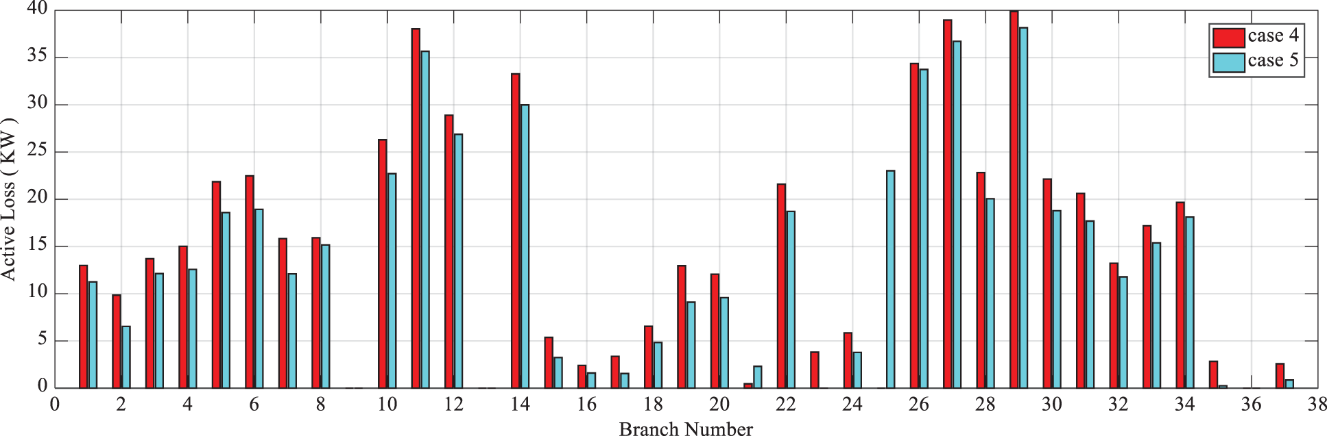
Figure 11: Active loss of branches in states 4 and 5 from the first scenario of the 33-bussystem

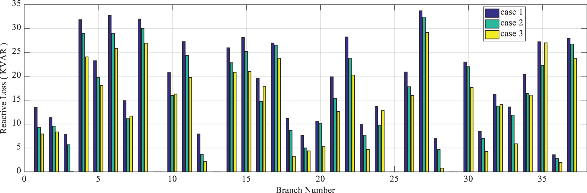
Figure 12: Reactive loss of branches in states 1, 2, and 3 from the first scenario of the 33-bus system

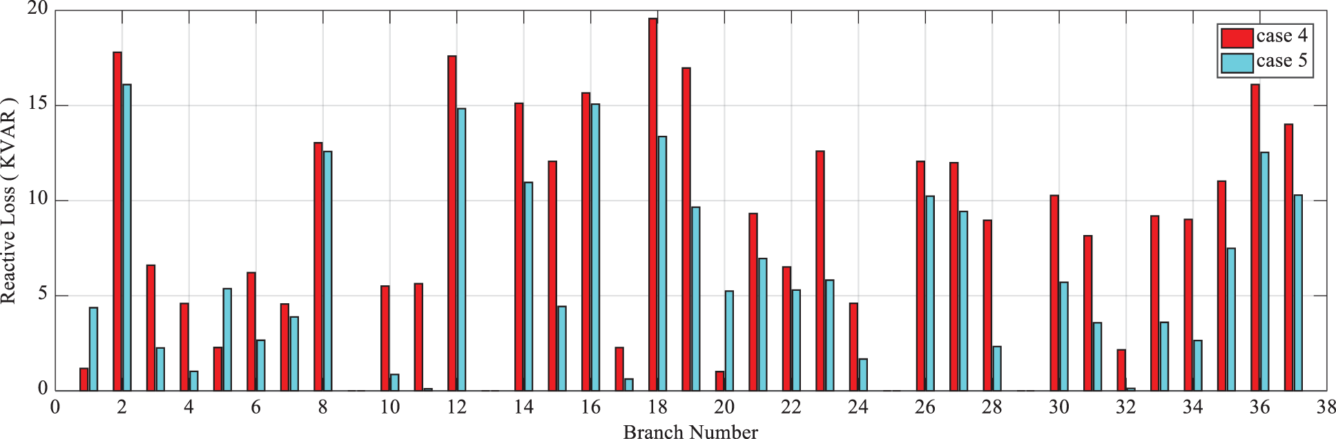
Figure 13: Reactive loss of branches in states 4 and 5 from the first scenario of the 33-bus system

4.3 Second Scenario

In the second scenario in the test 33-bus system, only the resource installed in bus 30 is modeled as PV and other resources are modeled as PQ. This scenario includes three objectives, namely loss reduction, improvement of voltage stability, and reduction of the number of switching operations. In this scenario, the following five states are investigated:

1) The initial system without reconfiguration and in the presence of DG with both PQ and PV models.

2) The system is reconfigured in such a way that the loss is reduced.

3) The system is reconfigured in such a way that the voltage stability index is improved or Eqs. (5)–(26) is reduced.

4) The system is reconfigured as in state 2 provided that the number of switching operations does not exceed four operations.

5) The system is reconfigured considering the compromise between all the above-mentioned objectives using the fuzzy-PSO method.

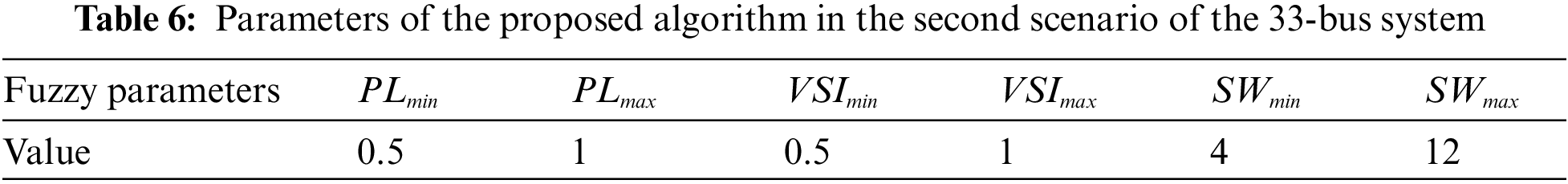
In this scenario, only some of the fuzzy parameters are changed as in Table 6.

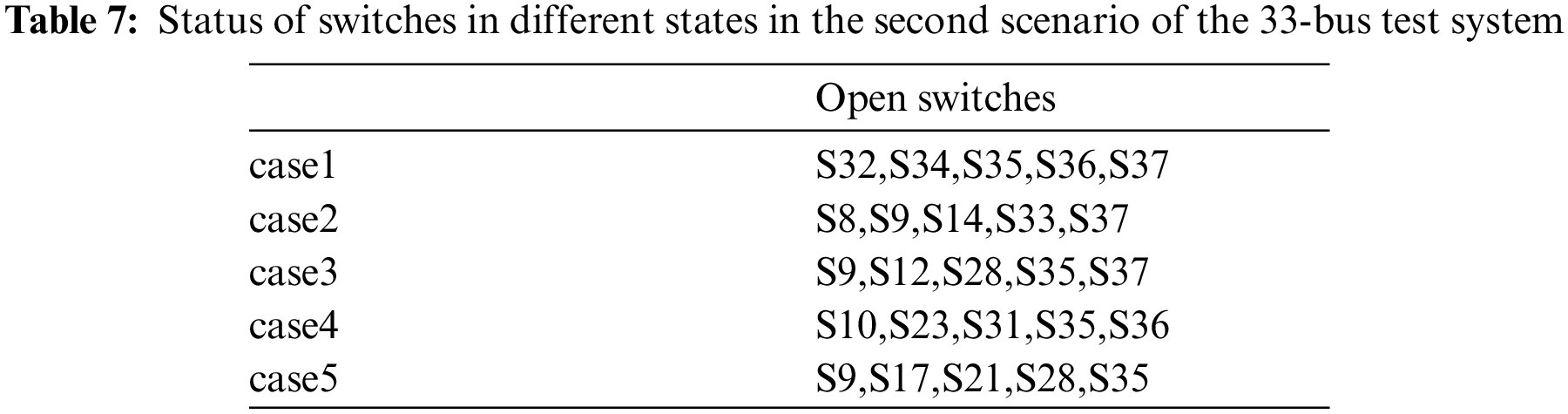
In this scenario in the 33-bus test system, as mentioned earlier, only the DGRs placed in bus 30 are modeled as PV in order to adjust the voltage of the intended bus on a per-unit system. But since the voltage of bus 30 in this system (i.e., the 33-bus test system) is very low, the DGR with its limitations in reactive power generation cannot adjust the voltage of the intended bus (bus 30) on a per-unit system. Regarding these points, the obtained optimal configuration and status of the switches in the studied five states are provided in Table 7.

As expected, the loss of the system exhibits maximum reduction in state 2 and the average voltage exhibits maximum increase in state 3. Also, the number of switching operations is minimized in state 4. But, in state 5, there is a compromise among the three objectives. In this state, although the loss is more than that in state 2, yet it exhibits more loss reduction than states 3 and 4. Moreover, in this state, although the average voltage does not improve exactly like that in state 3, yet it exhibits more improvement of the average voltage than other states. The reduction of the VS function indicates the improvement of the average voltage of the grid. Despite the number of the switching operation in state 5 is more than that in state 4, the power loss and VS function are reduced in state 5 compared to state 4. According to the Table 8, in none of the studied states, the DGR placed in bus 30 could set the voltage of the intended bus at a per-unit because it encounters its maximum generated reactive power. If the DG resource does not have the reactive power generation limitation (QGmax=400kvar), then, for example for state 2, the following results will be obtained, which are not satisfactory. The reason is that, in addition to the high generated reactive power of the DGR, the obtained results for the losses and minimum voltage are not undesirable compared to state 2.

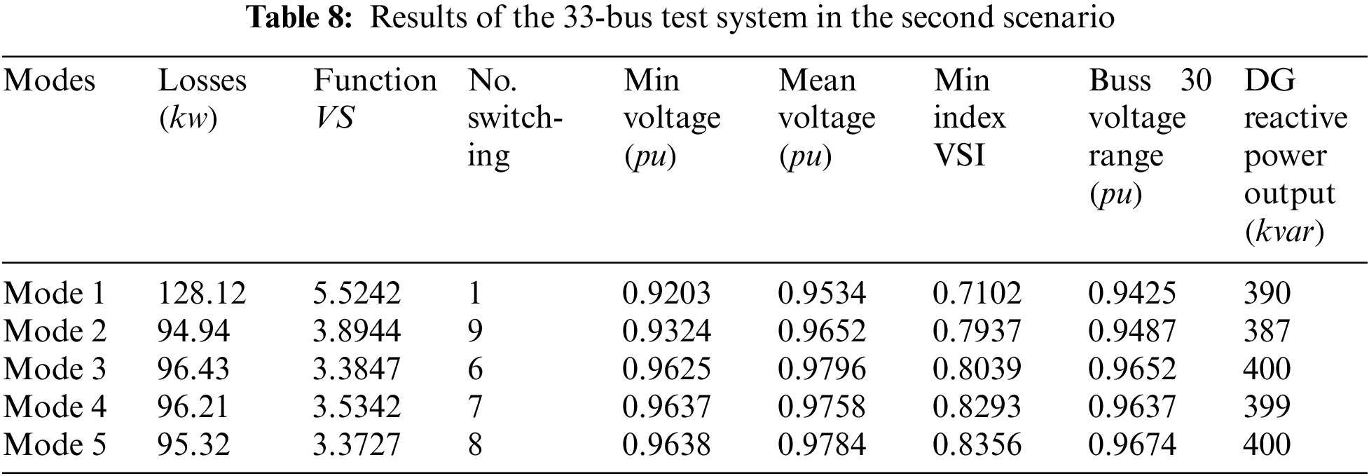
If in state 1, all four DGRs are modeled as PQ, the voltage domain of bus 30 will be obtained equal to 0.9324 per unit; thus, regarding the above table, the voltage domain of the intended bus will be improved in all the studied states compared to the state, in which the resource is modeled as PQ.

Below, the five studied states are compared in the voltage stability index. According to Fig. 14, the voltage stability index is improved in most of the buses in states 2 and 3, in which the reconfiguration is done, compared to state 1. The minimum and average values of VSI in state three are improved more than state 2; thus, considering this index, state 3 yields a better result in terms of voltage stability than states 1 and 2. As can be seen in this figure, the minimum and average values of the voltage stability of the buses in state five are improved compared to those in state 4. In-state 5, the minimum value of the VSI index is improved, even more than state 3. As expected, the average value of this index in state 3 is obtained bigger than state 5 because by optimizing (minimizing) the VS function in state 3, in fact, the average value of the voltage stability index of the buses is improved.

For a better presentation, Fig. 15 shows the 33-bus system changes after rearrangement.

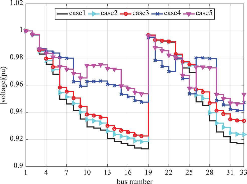
Figure 14: Voltage stability index of buses in states 1 to 5 from the second scenario of the 33-bus system

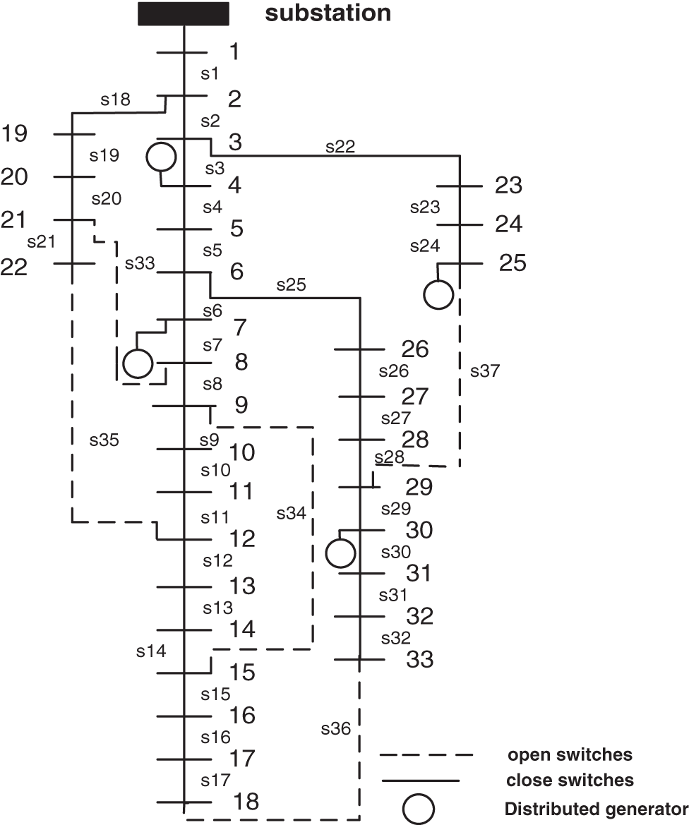
Figure 15: Single diagram of 33-bus test system in mode 1

4.4 Analysis of Convergence Speed of the Algorithm

In this section, the convergence speed of the proposed algorithm is investigated in comparison with other algorithms. To perform the simulation, the proposed algorithm was compared with the standard ABC algorithm, the PSO algorithm, and the GA. In fact, to investigate the performance of the algorithm, 30 different runs were considered. To provide identical conditions, the initial population was assumed equal for all, which was 50. The results of the convergence of the algorithm are presented in Table 9.

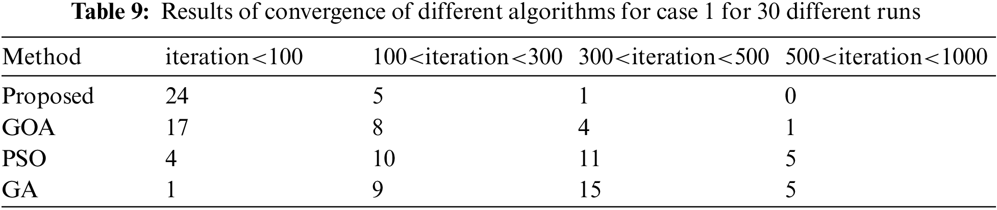
The results in the above table indicated the proposed algorithm had much better performance than other methods. the obtained results indicated lower standard deviation of the proposed algorithm in finding the optimal solution.

5  Conclusion

The distribution grid is a part of the overall structure of the power systems. It is known as the final phase of the chain of electric energy generation and transmission to the consumption point. This part of the system accounts for a significant portion of the power loss of the electricity network due to its specific features. One of the most cost-effective methods for reducing the losses is the reconfiguration of the distribution grid. Besides, adding the DG to the distribution grid causes the radial state of the grid and the one-sided passage of the power to be eliminated, and the ordinary and straightforward grid be replaced with a complex one. Thus, the DG affects the distribution system from different aspects. These effects can be positive or negative, depending on the conditions of the function and performance of the system as well as the capacity and location of the resources. One of the most essential things that can be affected by the DG in distribution grids is the issue of reconfiguration. DGs are the generation resources of electric energy connected to the distribution grid. These resources have lower size (volume) and generation capacity than the large generators and power plants and are operated with lower costs. The present paper aimed to solve the multi-objective problem of optimizing dynamic reconfiguration of distribution feeders in the presence of DGRs and ES units considering the uncertainty of the resources. The proposed optimization problem method was an improved self-adaptive PSO algorithm. The objective functions in this study included the non-distributed energy, energy losses, and voltage stability index. The simulation results indicated the superiority of the proposed method to other methods. The impact of the DG and ES resulted in the reduction of the losses and non-distributed energy as well as improvement of the voltage stability index of the grid. Considering the voltage stability index beside the non-distributed energy as the objective functions of the problem provided safe and acceptable conditions for the operation of the grid.

Funding Statement: This work was supported by The Training Plan of Young Backbone Teachers in Colleges and Universities of Henan Province (2018GGJS175: Research on Intelligent Power Management System).

Conflicts of Interest: The authors declare that they have no conflicts of interest to report regarding the present study.

References

 1.  Malekshah, S., Rasouli, A., Malekshah, Y., Ramezani, A., Malekshah, A. (2021). Reliability-driven distribution power network dynamic reconfiguration in presence of distributed generation by the deep reinforcement learning method. Alexandria Engineering Journal, 61(8), 6541–6556. DOI 10.1016/j.aej.2021.12.012. [Google Scholar] [CrossRef]

 2.  Khajehvand, M., Fakharian, A., Sedighizadeh, M. (2021). A risk-averse decision based on IGDT/stochastic approach for smart distribution network operation under extreme uncertainties. Applied Soft Computing, 107(1), 107395. DOI 10.1016/j.asoc.2021.107395. [Google Scholar] [CrossRef]

 3.  Huang, Y. C., Chang, W. C., Hsu, H., Kuo, C. C. (2021). Planning and research of distribution feeder automation with decentralized power supply. Electronics, 10(3), 362. DOI 10.3390/electronics10030362. [Google Scholar] [CrossRef]

 4.  Sarkar, D., Gunturi, S. K. (2021). Machine learning enabled steady-state security predictor as deployed for distribution feeder reconfiguration. Journal of Electrical Engineering & Technology, 16(3), 1197–1206. DOI 10.1007/s42835-021-00668-x. [Google Scholar] [CrossRef]

 5.  Singh, J., Tiwari, R. (2020). Electric vehicles reactive power management and reconfiguration of distribution system to minimise losses. IET Generation, Transmission & Distribution, 14(25), 6285–6293. DOI 10.1049/iet-gtd.2020.0375. [Google Scholar] [CrossRef]

 6.  Fakharian, A., Sedighizadeh, M., Khajehvand, M. (2021). Optimal operation of unbalanced microgrid utilizing copula-based stochastic simultaneous unit commitment and distribution feeder reconfiguration approach. Arabian Journal for Science and Engineering, 46(2), 1287–1311. DOI 10.1007/s13369-020-04965-x. [Google Scholar] [CrossRef]

 7.  Rawat, T., Niazi, K. R., Gupta, N., Sharma, S. (2021). Impact of responsive demand scheduling on optimal operation of smart reconfigurable distribution system. In: Recent Advances in Power Systems, pp. 117–125. Singapore: Springer. [Google Scholar]

 8.  Lotfi, H., Shojaei, A. A., Kouhdaragh, V., Amiri, I. S. (2020). The impact of feeder reconfiguration on automated distribution network with respect to resilience concept. SN Applied Sciences, 2(9), 1–14. DOI 10.1007/s42452-020-03429-z. [Google Scholar] [CrossRef]

 9.  Lotfi, H. (2020). Multi-objective energy management approach in distribution grid integrated with energy storage units considering the demand response program. International Journal of Energy Research, 44(13), 10662–10681. DOI 10.1002/er.5709. [Google Scholar] [CrossRef]

10. Azizivahed, A., Narimani, H., Fathi, M., Naderi, E., Safarpour, H. R. et al. (2018). Multi-objective dynamic distribution feeder reconfiguration in automated distribution systems. Energy, 147(2), 896–914. DOI 10.1016/j.energy.2018.01.111. [Google Scholar] [CrossRef]

11. Azizivahed, A., Narimani, H., Naderi, E., Fathi, M., Narimani, M. R. (2017). A hybrid evolutionary algorithm for secure multi-objective distribution feeder reconfiguration. Energy, 138, 355–373. DOI 10.1016/j.energy.2017.07.102. [Google Scholar] [CrossRef]

12. Abedinia, O., Amjady, N., Ghasemi, A., Hejrati, Z. (2013). Solution of economic load dispatch problem via hybrid particle swarm optimization with time-varying acceleration coefficients and bacteria foraging algorithm techniques. International Transactions on Electrical Energy Systems, 23(8), 1504–1522. DOI 10.1002/etep.1674. [Google Scholar] [CrossRef]

13. Naderi, E., Narimani, H., Fathi, M., Narimani, M. R. (2017). A novel fuzzy adaptive configuration of particle swarm optimization to solve large-scale optimal reactive power dispatch. Applied Soft Computing, 53, 441–456. DOI 10.1016/j.asoc.2017.01.012. [Google Scholar] [CrossRef]

14. Lotfi, H., Nikooei, A. S., Shojaei, A. A., Ghazi, R., Sistani, M. B. N. (2020). An enhanced evolutionary algorithm for providing energy management schedule in the smart distribution network. Majlesi Journal of Electrical Engineering, 14(2), 17–23. [Google Scholar]

15. Azizivahed, A., Lotfi, H., Ghadi, M. J., Ghavidel, S., Li, L. et al. (2019). Dynamic feeder reconfiguration in automated distribution network integrated with renewable energy sources with respect to the economic aspect. In: 2019 IEEE Innovative Smart Grid Technologies-Asia (ISGT Asia), pp. 2666–2671. Chengdu, China: IEEE. [Google Scholar]

16. Mahboubi-Moghaddam, E., Narimani, M. R., Khooban, M. H., Azizivahed, A. (2016). Multi-objective distribution feeder reconfiguration to improve transient stability, and minimize power loss and operation cost using an enhanced evolutionary algorithm at the presence of distributed generations. International Journal of Electrical Power & Energy Systems, 76(1), 35–43. DOI 10.1016/j.ijepes.2015.09.007. [Google Scholar] [CrossRef]

17. Murty, V. V. S. N., Kumar, A. (2021). Voltage regulation and loss minimization in reconfigured distribution systems with capacitors and OLTC in the presence of PV penetration. Iranian Journal of Science and Technology, Transactions of Electrical Engineering, 45(2), 655–683. DOI 10.1007/s40998-020-00389-3. [Google Scholar] [CrossRef]

18. Ameli, A., Ahmadifar, A., Shariatkhah, M. H., Vakilian, M., Haghifam, M. R. (2017). A dynamic method for feeder reconfiguration and capacitor switching in smart distribution systems. International Journal of Electrical Power & Energy Systems, 85(3), 200–211. DOI 10.1016/j.ijepes.2016.09.008. [Google Scholar] [CrossRef]

19. Sheidaei, F., Ahmarinejad, A., Tabrizian, M., Babaei, M. (2021). A stochastic multi-objective optimization framework for distribution feeder reconfiguration in the presence of renewable energy sources and energy storages. Journal of Energy Storage, 40, 102775. DOI 10.1016/j.est.2021.102775. [Google Scholar] [CrossRef]

20. Teng, J. H. (2003). A direct approach for distribution system load flow solutions. IEEE Transactions on Power Delivery, 18(3), 882–887. DOI 10.1109/TPWRD.2003.813818. [Google Scholar] [CrossRef]

21. Shirmohammadi, D., Hong, H. W., Semlyen, A., Luo, G. X. (1988). A compensation-based power flow method for weakly meshed distribution and transmission networks. IEEE Transactions on Power Systems, 3(2), 753–762. DOI 10.1109/59.192932. [Google Scholar] [CrossRef]

22. Olabi, A. G., Abdelkareem, M. A., Wilberforce, T., Sayed, E. T. (2021). Application of graphene in energy storage device--A review. Renewable and Sustainable Energy Reviews, 135(2), 110026. DOI 10.1016/j.rser.2020.110026. [Google Scholar] [CrossRef]

23. Venkatesan, Y., Palanivelu, A. (2021). Soccer game optimization-based power flow for distribution networks. COMPEL-The International Journal for Computation and Mathematics in Electrical and Electronic Engineering, 40(3), 456–474. DOI 10.1108/COMPEL-10-2020-0349. [Google Scholar] [CrossRef]

24. Song, B., Wang, Z., Zou, L. (2021). An improved PSO algorithm for smooth path planning of mobile robots using continuous high-degree Bezier curve. Applied Soft Computing, 100(1), 106960. DOI 10.1016/j.asoc.2020.106960. [Google Scholar] [CrossRef]

This work is licensed under a Creative Commons Attribution 4.0 International License, which permits unrestricted use, distribution, and reproduction in any medium, provided the original work is properly cited.