Energy Engineering

---

DOI: 10.32604/ee.2022.020005

ARTICLE

Prediction of Residential Building’s Solar Installation Energy Demand in Morocco Using Multiple Linear Regression Analysis

Nada Yamoul1,*, Latifa Dlimi1 and Baraka Achraf Chakir2

1Department of Physics, Faculty of Sciences, Ibn Tofail University, Kenitra City, 14000, Morocco
2Department of Mathematics, Faculty of Sciences, Ibn Tofail University, Kenitra City, 14000, Morocco
*Corresponding Author: Nada Yamoul. Email: yamoul.nada@gmail.com
Received: 29 October 2021; Accepted: 27 April 2022

1  Introduction

The world’ s energy resources are constantly being consumed at a speed that will lead to the exhaustion of non-renewable resources in the future. It is thus crucial to ensure rational and economic management of energy. With more than 3000 h/year of sunshine, and irradiation of 5 kWh/m2/day, Morocco has a significant capacity to produce solar energy.

In this regard, Morocco has adopted an energy strategy based on the development of renewable energy and energy efficiency, that aims to achieve a primary energy saving of about 12% by 2020 and 15% by 2030 [1]. To implement this strategy, an energy efficiency plan has been put in place covering all sectors, especially the building sector which has a significant source of energy savings. In this sense,the public authorities have undertaken a series of actions to optimize energy consumption and promote the use of renewable energy at the scale of housing and the city. Within these energy efficiency actions, we are concerned primarily with integrating solar heaters in housing.

The use of solar thermal energy to produce domestic hot water is one of the major challenges of the transition to energy-efficient buildings. It is a simple option to reduce fossil fuel consumption and GHG gas emissions. On the other hand, there is a lack of awareness of the opportunities that solar energy offers, both by the general population and by the actors of the construction sector.

1.1 Need for Research

In the residential sector, domestic hot water production can represent a significant percentage of the annual energy consumption. It is essential to note that heating, ventilation, air conditioning, lighting, and hot water systems account for more than two-thirds of the buildings’ energy consumption as is shown in Fig. 1 according to the Moroccan Agency of Energy Efficiency (AMEE) [2]. Nevertheless, the thermal regulation has not established the minimum energy performance integrating the building and its equipment. Also, it has not included requirements regarding the installation or production of energy generated by renewable sources which may be integrated into the structure of the building.

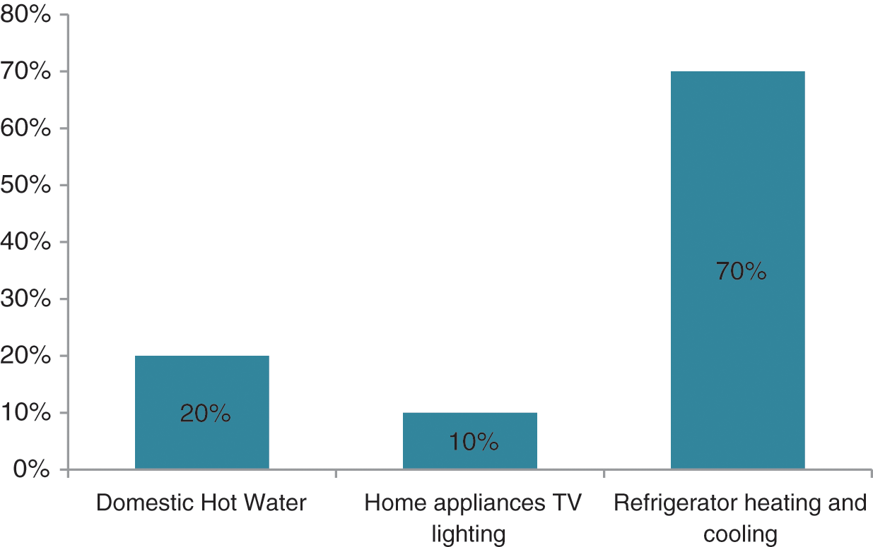
Figure 1: Distribution of energy used in housing in morocco according to energy and energy efficiency (AMEE)

For the collective housing buildings located in the Mediterranean climate, the production of domestic hot water can represent nearly 25% [3] of the energy bill of the dwellings.

However, the integration of solar renewable energy systems in buildings faces several challenges such as:

•   Lack of standardized financial products for energy-efficient buildings and energy renewable energy equipment;

•   Lack of awareness among households, retailers, financial institutions and real estate developers of the benefits of energy efficiency and renewable energy equipment [4];

•   Lack of technical standards and guidelines to support the implementation of existing framework laws for energy efficiency and renewable energy buildings and equipment [4];

•   Low prices of conventional energies such as gas and electricity which are heavily subsidized, thus limiting the solar alternative in terms of reducing the energy bill.

1.2 Research Objectives

The objectives of this research are as follows:

•   Promote the installation of solar water heaters in the collective building in Morocco by proposing implementation measures adapted to the Moroccan context.

•   Estimate the needs for domestic hot water and define the characteristics of the solar installation.

2  Literature Review

2.1 Predictions Models

The development of thermal models is an integral part of the design process, particulary demonstrating compliance with the building regulations [5]. Thermal modeling of the building is essential for calculating energy needs for simulation or prediction [6]. The development of tools for simulating energy performance in buildings makes it possible to have detailed models taking into account current knowledge of physical phenomena in interactions in the building (envelope, insulation, joinery, treatment of thermal bridges, systems, fluids, etc…).

The field of research relating to the modeling of buildings and the prediction of energy performance involves several scientific fields, namely fields related to physics, focusing on the resolution of equations simulating the thermal behavior of the building, and those related to mathematics, consisting of the implementation of a prediction model using machine learning techniques.

In this perspective, the specificity of statistical models as compared to physical methods is the absence of physical information. No thermal or geometrical parameters; and no heat transfer equations are required beforehand. The statistical models are essentially based on the implementation of a function inferred from training data samples representing the behavior of a specific system.

Therefore, such methods are well suited when the physical characteristics of the studied building are not available. Various statistical techniques are able to generate a predictive model through learning methods. The major power of these tools resides in the fact that they do not necessitate an extensive knowledge of the building geometry or complex physical phenomena to extract an appropriate prediction model. On the other hand, they are completely metrics-based and in cases where collecting data is challenging, this can become a real problem.

Prediction models are generally grouped into three categories: “white box” models, “black box” models and “grey box” models [7]. The first is a physical technique and is divided into three different tools depending on the characteristics of the construction. The “white box” [7] models described the system explicitly, they are deterministic or knowledge models built from the physical laws that govern the phenomena involved in the studied system. They allow reproduction of the dynamics of the buildings but can become very heavy and time-consuming, which is not compatible with a real-time application.

The second, “black box” model [8], allowes a digital resolution of the problem without providing any physical interpretation of the system studied. These are empirical models built based on measurements and input/output relationships; they require measurements over a long period to predict the behavior of the building under several conditions. And finally, the “gray box” models or semi-physical models combine the physical sense and the spirit of simple models. These are hybrid models corresponding to semi-physical modeling, which considers the knowledge and the measurements while remaining of reduced size for a better compromise with the control application (methods of electrical analogy). This category of models consists of the modeling of the building envelope by electrical analogy, which makes it possible to understand the structure of the model by a rapid observation of the equivalent electrical circuit.These models imply the knowledge of thermal parameters, such as capacitance and thermal resistance of different orders [9].

2.2 The Chosen Approach for Thermal Modeling

The multiple linear regression model is the most common statistical tool used to study multidimensional data [9]. It is a special case of a linear model and is the natural generalization of simple regression. The purpose of simple multiple regression is to explain a variable Y with the help of a variable X(X1,…,Xq).

The variable Y is called the dependent variable, or variable to be explained and the variables Xj (j = 1,…, q) are called independent variables, or explanatory variables.

We consider that an endogenous variable is explained by a single exogenous variable, but it is extremely rare that a single variable can explain an economic or social phenomenon. The general linear model generalizes the simple regression model with several explanatory variables.

∀t=1…nyt=a0+a1x1t+a2x2t+a3x3t+…+anxnt+εt(1)

yt: Variable to be explained at date t and xit: Explanatory variable i at date t;

a0, …, an: Parameters of the model and n: number of observations;

εt = specification error (difference between the true model and the specified model).

Assumptions and properties of estimators

By construction, the model is linear in X (or on these coefficients) and we distinguish stochastic assumptions (related to the error ε) from structural assumptions.

- H1: the values XI,t are observed without error.

- H2: E(εt) = 0, the mathematical expectation of the error is zero.

- H3: E(εt2) = σ2, the variance of the error is constant ∀t) (homoscedasticity).

- H4: E(εtεt′) = 0 if t ≠ t′, the errors are uncorrelated (or independent).

- H5: Cov (xit, εt) = 0, the error is independent of the explanatory variables.

With Cov (xit, εt): the covariance between xit and εt.

2.2.1 Matrix Form

The previous writing of the model is not very practical [10]. To simplify the writing of the model and to facilitate the expression of specific results, we usually use matrix notation. By writing the model, observation by observation, we obtain:

y1=a0+a1x11+a2x21+a3x31+…+akxk1+ε1(2)

y2=a0+a1x12+a2x22+a3x23+…+anxk2+ε2(3)

yn=a0+a1x1n+a2x2n+a3x3n+…+anxkn+εn(4)

Let Y,in matrix form:Y=Xa+ε(5)

With Y=(y1..yn) , X=(1x11.xk1........1x1n.xkn) and a=(a1..an) ε=(ε1..εn)

We notice the first column of the matrix X, composed of 1, which corresponds to the coefficient a (coefficient of the constant term). The dimension of the matrix X is therefore n rows and k + 1 columns (k being the number of real explanatory variables, i.e., constant excluded).

2.2.2 Estimation and Properties of Estimators

Let the model be in matrix form with k explanatory variables and n observations, represented by the Eq. (5):

Y=Xa+ε

To estimate the vector a composed of the coefficients a0,…an, we apply the Ordinary Least Squares (OLS) method which consists in minimizing the sum of the squares of the errors:

Min∑t=1nεt2=Minε′ε=Min(Y−Xa)(Y−Xa)′=MinS(6)

With ε′ transpose1 of vector ε.

To minimize this function concerning a, we differentiate 2 S with respect to a:

dsda=−2X′Y+2XX′a^(7)

Soa^=(X′X)−1X−Y(8)

This solution is feasible if the square matrix X′X of dimension (k + 1, k + 1) is invertible. The matrix X′X is the cross-product matrix of the explanatory variables; in the case of perfect collinearity between two explanatory variables, the matrix X' X is singular and the OLS method fails [11]. The equations derived from the relationship:

X′Xa^=X′Y(9)

The estimated model is written:

yt=a^0+a^1x1t+a^2x2t+a^3x3t+…+a^nxnt(10)

With et = yt − y^t where et is the residual, i.e., the difference between the observed value of the variable to be explained and its estimated (adjusted) value.

2.2.3 The Generalized Least Squares Method

Consider the general linear model: Y=Xa+ε, in which E(ε′ε)=Ωε≠σε2I (Ωε is of dimension n * n)).

We want to determine an estimator that has the same properties as the OLS estimator [12]: unbiased, linear function of Y, and minimum variance. This allows us to best explain the data, and that is exactly what the ordinary least squares method allows us to do. Indeed, suppose that E ([X]) E (ε[X]) = 0 and V (ε[X]) = Σ which is the covariance matrix of the residuals. Then, it is shown that this estimator is given by:

a^=(X′Σ−1X)−1(X′Σ−1X) andΩε=(X′Σ−1X)−1(11)

This estimator is called the Generalized Least Squares (GLS) estimator or the Aiken estimator.

2.2.4 Special Case: The Simple Regression Model

Linear regression is a statistical method used to predict the response of certain systems to their input factors using polynomial models [13]. It was introduced by Francis Galton in 1886. Several mathematical models can be used to predict Energy Demand in buildings.

Indeed, Eq. (12) is the linear model; many authors use it, as we will present below. This model gives satisfactory results as a function of its correlation coefficient and assumes the linear relationship between the vector of input factors [X] and the response vector [Y]. The linear models take into account the interaction between the first and second-order factors, respectively. They can be used to add precision to the response [Y] when independent parameters [X] interact with each other. Finally, the quadratic model represented by Eq. (14) is used by adding a pure quadratic term to the linear term in order to focus the response and optimize the prediction.

The multilinear model accurately predicts the Energy Demand of buildings in different climates. This model will be used in the case of application.

Y=b0+∑i=1nXi(12)

Y=b0+∑i=1nbiXi∑i,j=1nb¯ijXiXj(13)

Y=b0+∑i=1nbiXi∑i,j,k=1nb¯ijkXiXjXk(14)

Y=b0+∑i=1nbiXi∑i,=1nb¯iiXi2(15)

In addition, in the linear model, the Durbin-Watson (DW) [14] criterion accounts for the autocorrelation of the absolute errors (residuals ei); which represents the difference between the value of the response estimated by the model and that calculated by simulation. The DW criterion is given by the Eq. (16): The DW value converges to zero in the case of a strong correlation between successive points. If there is a weak correlation between successive points, a random distribution of the error, the DW value is closer to 2.

DW=∑i=1N(ei−1−ei)2∑i=1Nei2(16)

3  Methodology

This research aims to develop a comprehensive understanding of building thermal modeling approaches used to identify energy savings or efficiency of buildings. In order to achieve this aim, firstly, a literature review on the various prediction models has been done. The study of the parameters of the different categories has been described during this phase to select the appropriate approach to be used during the modeling and simulation phase.

Secondly, this has been followed by presenting the chosen prediction model “black box”, which refers to a regression model for predicting the monthly energy requirement of a solar installation.

Lastly, the different results obtained during the study have been analyzed and suggestions on the selected solutions have been made.

3.1 Research Approach

3.1.1 Phase 1: Development of-the-Black-Box Model Based on Multiple Linear Regression Analysis

In this part, we have tried to model the energy need of the city of Casablanca during the year. Based on a multiple regression model.

The regression method attempts to determine the values taken by a variable while taking into account the influence of the other variables. We will then say that there is a dependent variable and several independent variables. The model equation is written as:

∀i∈[1,n]Yt=b0+b1x1i+b2x2i+ei(17)

The calculation method adopted as shown in Fig. 2 can be represented as a black box in which we introduce some parameters: Meteorological data, System data. The method allows for the output of both Solar Production and Energy Demand.

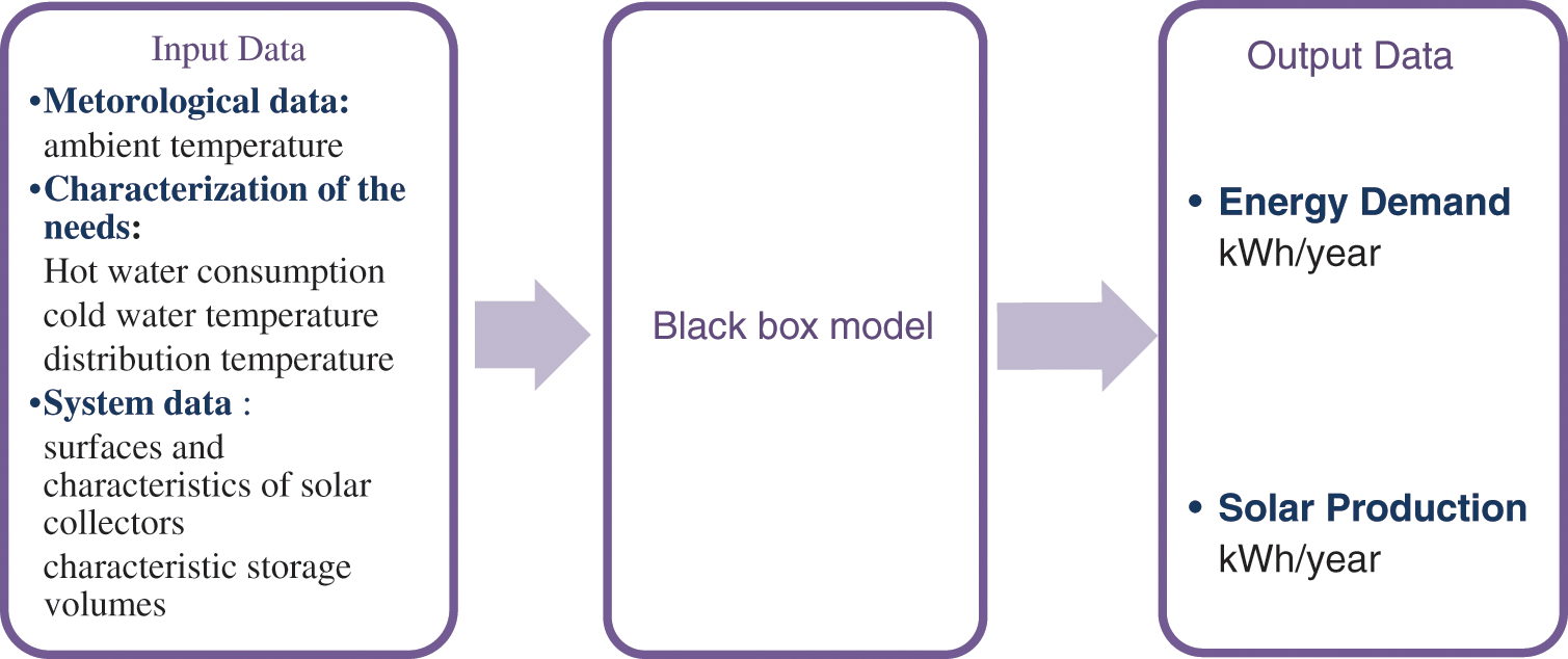
Figure 2: Schematic diagram of the calculation method

In general cases, the performance of a solar installation is characterized by two criteria: the “solar production”, the energy production of the installation in (kWh/year), and the “solar coverage rate” in (%), which is determined as the ratio of the solar production to the Energy Demand of the hot water station.

3.1.2 Phase 2

Building description

The existing building subject of the study is a collective housing building, located in Casablanca.

Location

The choice of the location must satisfy several different parameters. To get the maximum amount of sunlight, you must take into account.

- The orientation of the collectors;

- The inclination of the collectors;

- The risks of shading on the collectors.

Parameters

- Latitude of Casablanca: 33°34;

- Number of housing 16;

- Number of persons from 4 to 6 persons per housing;

- Installation:

•   The surface of solarcollectors: 70 m²

•   The inclination: 30/Horizontal

•   The orientation: 0/South

The data collection was conducted based on the meteorological stations and the description of the building’s characteristics: the location of the building, the number of occupants. In addition, we have used a calculation tool SOLO 2000 [15] in order to dimension solar thermal installations and determine their pefomances. The SOLO method has been ported to several easy-to-use computer applications and provides access to weather data from a large number of countries. This application was developed with the support of The Agency for Ecological Transition (ADEME ) [16] about ten years ago.

The Table 1 represents the global calculation results of the simulation to cover the needs in terms of domestic hot water.

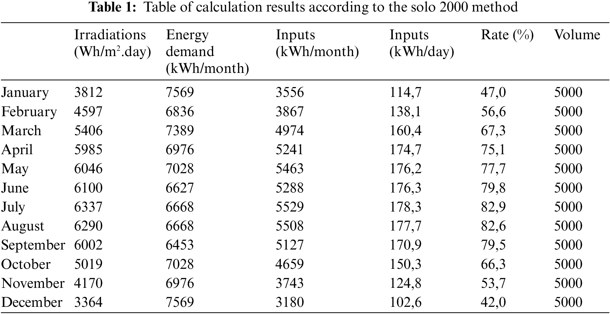
The Energy Demand in domestic hot water of the same dwelling can vary from one month to another according to the nature of the data used: volumes consumed, outdoor and cold water temperatures. For the months of December and January, with lower solar irradiation values, high values are recorded in terms of Energy Demand, contrary to the months of July and August, for example, where a high value of irradiation is recorded, which implies a decrease in the Energy Demand.

Table 2 shows some main indicators to measure the performance of the solar system.

3.1.3 Phase 3

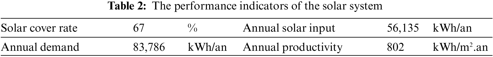
The graph in Fig. 3, shows in the upper part, the energy needs, the solar production and the coverage rate for a surface. It can be seen that the needs decrease in summer, while the solar production and the coverage rate of the collectors increase. The coverage rate is about 80% in summer. It is necessary to be vigilant with the collectors’s surface to avoid exceeding the needs and provoking a real risk of overheating the collector.

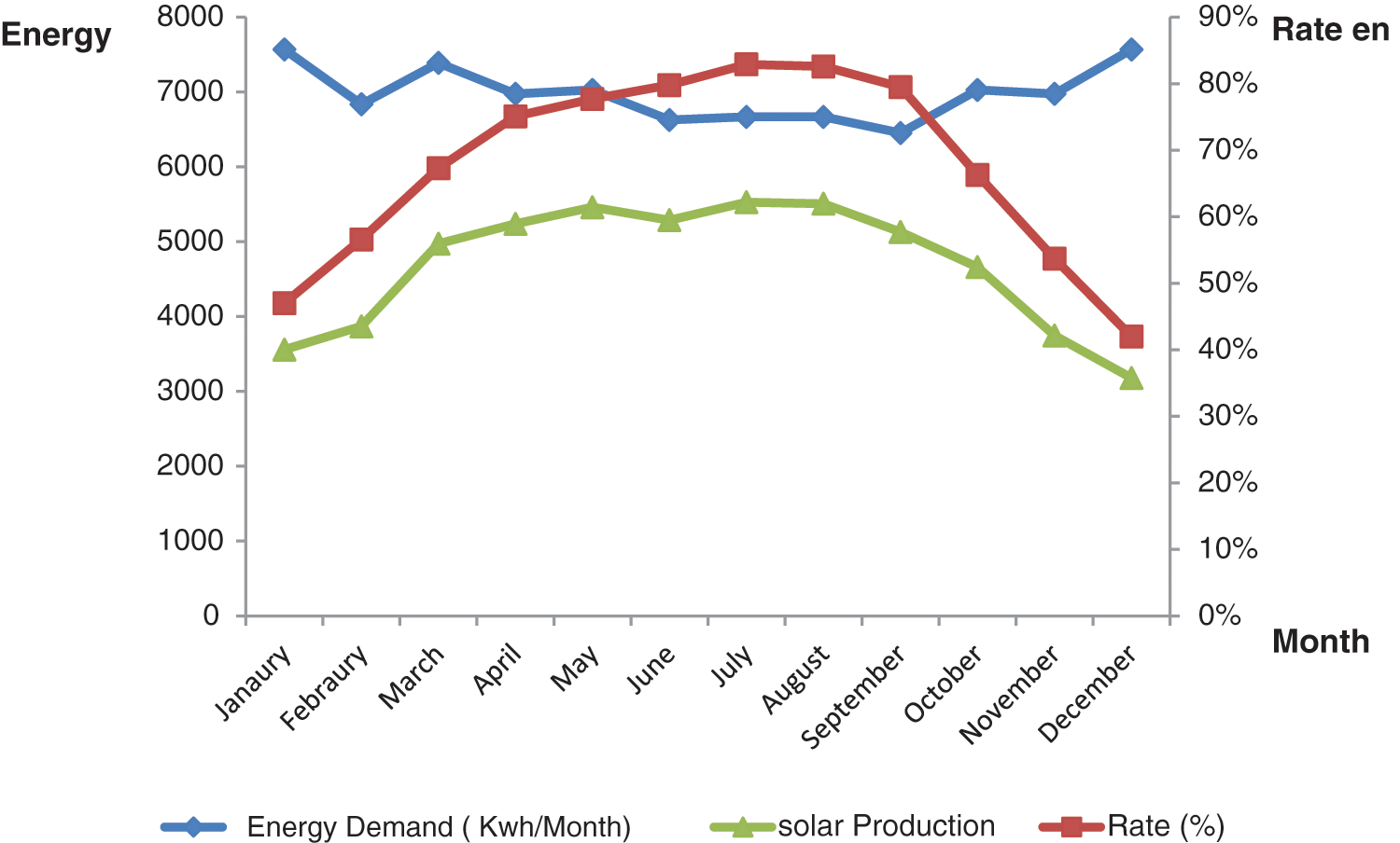
Figure 3: Theoretical energy balance of the solar installation of the reference building in Casablanca City

4  Analysis and Results of Multiple Regression Models

First, all available data were used to develop the model. Then, a selection of predictors was conducted, based on the p-value that gives an idea of the statistical significance of the variable in concern. The confidence interval was set at 5% and, therefore, all variables with a p-value less than 0.05 were eliminated.

4.1 Impact of Fluctuations in Endogenous Variables on Energy Requirements

The coefficient of determination is equal to 0,82, 0,98 for the models without constant terms and constant, hence the need to choose the model that maximizes R2.

The coefficient of determination (R² is the linear correlation coefficient r) is an indicator to assess the ability of a single or multiple linear regression. If the R² is close to 1, it indicates that the regression line equation is likely to determine 100% of the variation of the explanatory variables.

R2=0,98, very close to 1, means that the monthly intake and the average daily Irradiation explain 98% of the total variation in Energy Demand.

There are strong positive correlations between Energy Demand and Solar Gain, furthermore. There is a negative correlation between Energy Demand and Solar Irradiation, as mentioned by the scatter plot in Fig. 4.

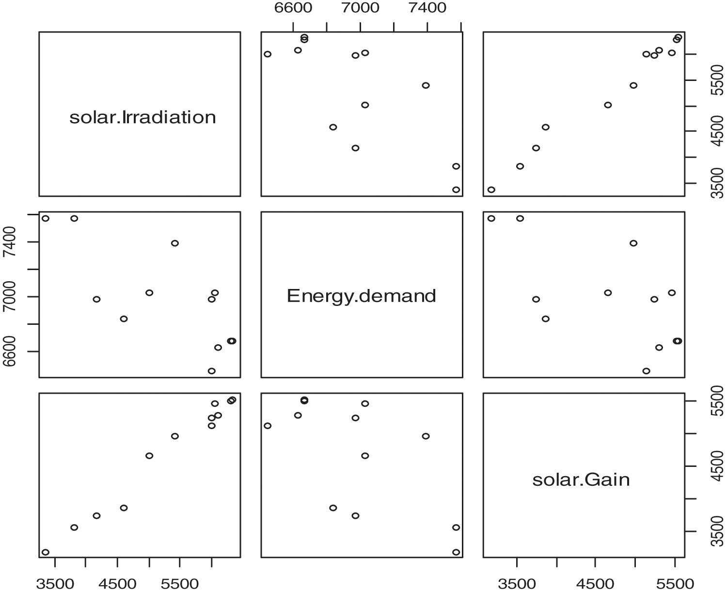
Figure 4: Scatter plots between solar gain, solar irradiation and energy demand

It has been proven that there is a significant relationship between Energy Demand and Solar Gain. The p-value of the Irradiation variable is 0,00124, which is less than 0,01, so there is evidence for the alternation hypothesis.

The Energy Demand equation as a function of Solar Gain and Solar Irradiation is written as:

EnergyDemand=7725,86+(1,46∗SolarGain)−(1,44∗Solarirradiation)(18)

In the long term, we observe that the monthly Energy Demand is significantly sensitive to the monthly Solar Gain and the average daily Solar Irradiation of sensors. Increasing the monthly Solar Gain by one unit generates a 1,509 increase in monthly Energy Demand. Otherwise, the increase in daily Solar Irradiation of sensors will decrease Energy Demand by 1,528.

The results show that increased Solar Irradiation of sensors implies a decrease in energy consumption, which means a decrease in Energy Demand.

There are strong positive correlations between Energy Demand and Irradiation, mentioned by the scatter plot in Fig. 4. It is concluded that the p-value of the Irradiation variable is 0,00368 which is less than 0,01. The p-value of the variable Irradiation is 0,00124; this, is less than 0,05 (5%) so there is evidence of the alternation hypothesis: there are negative correlations between Energy Demand and solar irradiation.

4.2 Residual Study

Residual: The residual (e) is a measure obtained [17], as a difference, between the real value of the dependent variable (target) (y) and the value predicted value (ŷ) using a model. Each data point has a residue. The sum and average of the residuals in a regression model are almost equal to zero.

Residual=Observedvalue−Predictedvalueore=y−y^(19)

The examination of the residuals is an essential step in linear regression. This step relies mainly on graphical methods proposed by the R software.

The Moustache Box, is a simple diagram used to represent the distribution of a variable. This diagram is composed of a rectangle that lies between the first and third quartile. The rectangle is divided by a line that corresponds to the median.

The purpose of the whisker box is to represent the center and distribution of the data. It is also a visual tool for checking normality or for identifying points that could be outliers or extremes.

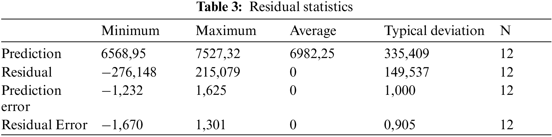
Table 3 presents statistics related to residuals, which is an important tool for checking whether a multiple regression has achieved its objective, while explaining as much variation as possible in a dependent variable. It confirms that the mean of the residuals is equal to 0, which confirms the hypotheses (H1, H2 cited before). Moreover, the analysis of the residuals made it possible to have a global vision of what remains after having explained the variation of the dependent variable, that is to say the unexplained variance.

The continuous black horizontal line, in our case, represents the median. Fig. 5 shows that the average of the residuals is equal to 0.

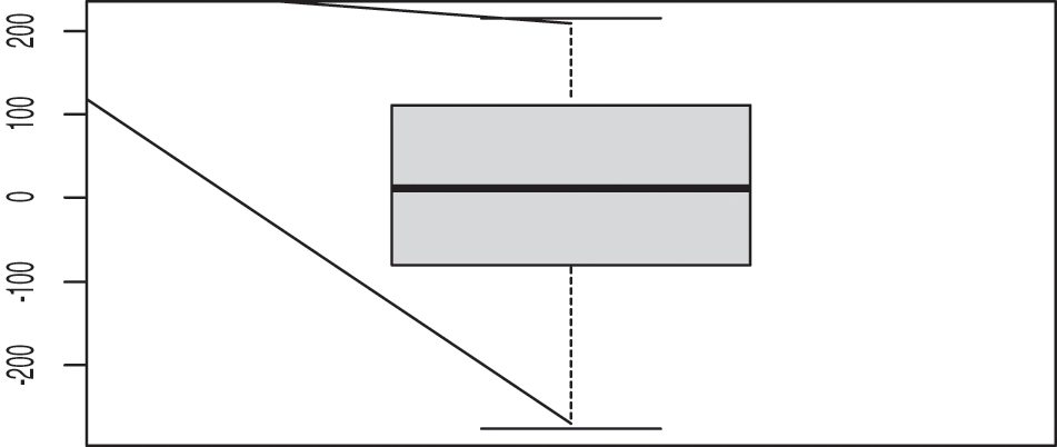
Figure 5: Box plot of residual

The residuals test has been well revised as shown in Table 3 above , and we even added the residuals statistics table in order to show that the mathematical expectation of the residuals is zero.

4.3 Estimation of the Energy Demand Model

The figure shows the comparison between the evolution of the Energy requirement and the estimate Energy Demand by the multiple regression model.

The graph in Fig. 6 represents the evolution of Energy Demand and the Estimate Energy Demand, we can see that the evolutions are almost similar and this is due to the reduced error term, which proves that the model is good.

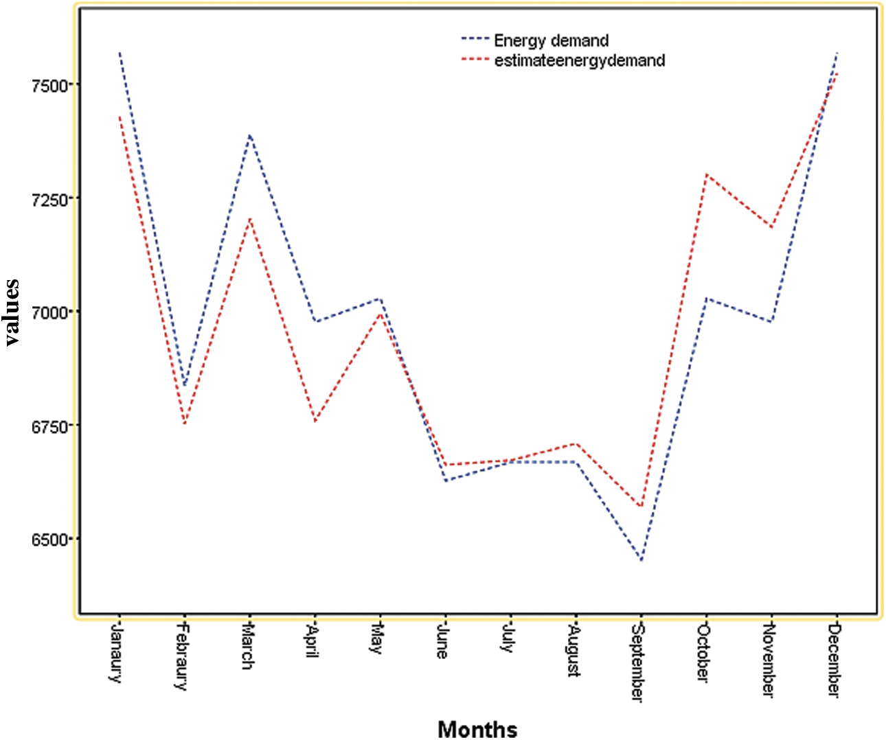
Figure 6: Evolution of energy demand and estimate energy demand

The coefficient of determination is equal, respectively to 0,82 for the models without term constant and 0,98 for the models with constant. From where the need to choose the model that maximizes R2.

R2 = 0,98 very close to 1, means that the monthly intake and the average daily irradiation Sensors can explain 98% of the total variation in Energy Demand.

5  Discussion and Conclusions

Morocco’s climatic conditions are exceptionally suitable for taking advantage of solar energy. The regions where most of the country’s population is located have solar radiation of more than 1800 kWh/m² per year, a resource more than able to cover a large part of the domestic hot water needs of the residential sector.

The use of solar energy for the production of domestic hot water in the collective residential sector in Morocco is only starting, and the number of achievements is still tiny.

This paper has provided a description of the main approaches to modeling the thermal behavior of buildings. We have proposed a review of black-box, white-box, and gray-box building system modeling approaches and prediction methods for improving the energy efficiency of buildings. The proposed approaches lead to mathematical models that can be used for the calculation of overall energy consumption; and energy demand in buildings.

The aim of this study is to develop a simple model allowing a user to predict the Energy Demand of a solar installation in Casablanca, without going through complex physical models. As demonstrated by the results above, the multiple linear regression allows having results quite acceptable, with an average absolute error percentage of less than 5%. Thanks to its simplicity of implementation and speed.

It should be noted that many elements must be taken into account in the design and implementation of a solar installation in a residential building: domestic hot water needs, meteorological data, and the objectives of solar coverage sought.

The most effective way to increase the use of Solar Energy in the residential sector would be to generalize this type of installation in new buildings, by requiring the consideration of this technology from the design phase and undertaking the appropriate measures to encourage the progressive generalization of these installations to all existing buildings. Among these measures, we can mention regulatory measures such as the development of national, and regional regulation for the obligation of solar thermal, direct financial incentives (direct subsidy), also the promotion of a mature market of solar thermal considering the real needs of households and finally the emergence and strengthening of a culture of energy efficiency in the building sector.

Funding Statement: The authors received no specific funding for this study.

Conflicts of Interest: The authors declare that they have no conflicts of interest to report regarding the present study.

References

 1.  Choukri, K., Naddami, A., Hayani, S. (2017). Renewable energy in emergent countries: Lessons from energy transition in Morocco. Energy, Sustainability and Society, 7(1), 1–11. DOI 10.1186/s13705-017-0131-2. [Google Scholar] [CrossRef]

 2.  Gargab, F. Z. (2021). Technical-economic optimization and manufacture of a Moroccan solar water heater (Doctoral Dissertation). Université de Pau et des Pays de l’Adour; Université Sidi Mohamed ben Abdellah (Fès, Maroc). Faculté des sciences. [Google Scholar]

 3.  Official Site of the Moroccan Agency for Energy Efficiency (AMEE). https://www.amee.ma/. [Google Scholar]

 4.  Mohamed, B. (2017). Les stratégies de développement durable en efficacité énergétique au Maroc. https://idl-bnc-idrc.dspacedirect.org/bitstream/handle/10625/58969/IDL%20-%2058969.pdf?sequence=2 [Google Scholar]

 5.  Barone, G., Buonomano, A., Forzano, C., Palombo, A. (2021). Implementing the dynamic simulation approach for the design and optimization of ships energy systems: Methodology and applicability to modern cruise ships. Renewable and Sustainable Energy Reviews, 150, 111488. DOI 10.1016/j.rser.2021.111488. [Google Scholar] [CrossRef]

 6.  Debbarma, M., Sudhakar, K., Baredar, P. (2017). Thermal modeling, exergy analysis, performance of BIPV and BIPVT: A review. Renewable and Sustainable Energy Reviews, 73(8), 1276–1288. DOI 10.1016/j.rser.2017.02.035. [Google Scholar] [CrossRef]

 7.  Amara, F., Agbossou, K., Cardenas, A., Dubé, Y., Kelouwani, S. (2015). Comparison and simulation of building thermal models for effective energy management. Smart Grid and Renewable Energy, 6(4), 95–112. DOI 10.4236/sgre.2015.64009. [Google Scholar] [CrossRef]

 8.  Berthou, T., Stabat, P., Salvazet, R., Marchio, D. (2014). Development and validation of a gray box model to predict thermal behavior of occupied office buildings. Energy and Buildings, 74(3), 91–100. DOI 10.1016/j.enbuild.2014.01.038. [Google Scholar] [CrossRef]

 9.  Afram, A., Janabi-Sharifi, F. (2015). Gray-box modeling and validation of residential HVAC system for control system design. Applied Energy, 137, 134–150. DOI 10.1016/j.apenergy.2014.10.026. [Google Scholar] [CrossRef]

10. Kumar, V., Vardhan, H., Murthy, C. S. (2020). Multiple regression model for prediction of rock properties using acoustic frequency during core drilling operations. Geomechanics and Geoengineering, 15(4), 297–312. DOI 10.1080/17486025.2019.1641631. [Google Scholar] [CrossRef]

11. Francq, B. G., Govaerts, B. B. (2014). Measurementmethods comparison with errors-in-variables regressions. From horizontal to vertical OLS regression, review and new perspectives. Chemometrics and Intelligent Laboratory Systems, 134, 123–139. [Google Scholar]

12. Variyath, A. M., Brobbey, A. (2020). Variable selection in multivariate multiple regression. PLoS One, 15(7), e0236067. DOI 10.1371/journal.pone.0236067. [Google Scholar] [CrossRef]

13. Marques, F. S., Grisi-Filho, J. H., Amaku, M., Silva, J. C., Almeida, E. C. et al. (2020). HybridModels: An R package for the stochastic simulation of disease spreading in dynamic networks. Journal of Statistical Software, 94(6), 1–32. DOI 10.18637/jss.v094.i06. [Google Scholar] [CrossRef]

14. Turner, P. (2020). Critical values for the Durbin-Watson test in large samples. Applied Economics Letters, 27(1495), 1499–1261. DOI 10.1080/13504851.2019.1691711. [Google Scholar] [CrossRef]

15. Agir, C. P. (2008). Production d’eau chaude sanitaire par énergie solaire. http://bamama.free.fr/196_Ico_guide.pdf. [Google Scholar]

16. Février, P. (2012). L’ADEME: Entre maîtrise de l’énergie et développement durable. Annales Historiques de Lelectricite, 10(1), 55–59. DOI 10.3917/ahe.010.0055. [Google Scholar] [CrossRef]

17. Baek, J. W., Chung, K. (2020). Context deep neural network model for predicting depression risk using multiple regression. IEEE Access, 8, 18171–18181. DOI 10.1109/ACCESS.2020.2968393. [Google Scholar] [CrossRef]

This work is licensed under a Creative Commons Attribution 4.0 International License, which permits unrestricted use, distribution, and reproduction in any medium, provided the original work is properly cited.