| Energy Engineering |
DOI: 10.32604/ee.2022.020011
ARTICLE
Distributionally Robust Optimal Dispatch of Virtual Power Plant Based on Moment of Renewable Energy Resource
Nanjing Power Supply Company of State Grid Jiangsu Electric Power Co., Ltd., Nanjing, 210019, China
*Corresponding Author: Yong Wang. Email: wangyongnjj@126.com
Received: 29 October 2021; Accepted: 12 January 2022
Abstract: Virtual power plants can effectively integrate different types of distributed energy resources, which have become a new operation mode with substantial advantages such as high flexibility, adaptability, and economy. This paper proposes a distributionally robust optimal dispatch approach for virtual power plants to determine an optimal day-ahead dispatch under uncertainties of renewable energy sources. The proposed distributionally robust approach characterizes probability distributions of renewable power output by moments. In this regard, the faults of stochastic optimization and traditional robust optimization can be overcome. Firstly, a second-order cone-based ambiguity set that incorporates the first and second moments of renewable power output is constructed, and a day-ahead two-stage distributionally robust optimization model is proposed for virtual power plants participating in day-ahead electricity markets. Then, an effective solution method based on the affine policy and second-order cone duality theory is employed to reformulate the proposed model into a deterministic mixed-integer second-order cone programming problem, which improves the computational efficiency of the model. Finally, the numerical results demonstrate that the proposed method achieves a better balance between robustness and economy. They also validate that the dispatch strategy of virtual power plants can be adjusted to reduce costs according to the moment information of renewable power output.
Keywords: Virtual power plant; optimal dispatch; uncertainty; distributionally robust optimization; affine policy
Renewable energy sources, including wind farms and photovoltaic arrays, have experienced explosive growth during the past few years. Besides, the transformation from centralized energy resources to distributed energy resources has become an evitable trend, owing to the advantages of distributed energy resources such as reliability, economy, flexibility, and environment friendly. However, serious problems also exist for distributed energy resources, such as small capacity, geographical dispersion, and stochastic power output, which present great challenges to the effective control of electric power systems. These risks can be mitigated by an effective technology called virtual power plants. Virtual power plants are aggregate portfolios to manage different types of distributed energy resources, such as conventional generation units, renewable energy sources, storages, and load demands, through advanced communication, measurement, and control techniques [1,2]. Such aggregation enables distributed energy resources with complementary advantages to improve the overall stability and realize the scale merit. The resulting aggregation also enables distributed energy sources with adequate dimensions to participate in electricity markets as an integrated entity, which provides the opportunity for the owners of distributed energy resources to seek more profits [3]. In this context, virtual power plants have been developed rapidly in recent years, making the utilization of distributed energy resources more flexible, adaptive, and profitable [4].
The randomness and uncertainty of renewable power output in virtual power plants have posed severe challenges to the safe and stable operation of electric power systems. Extensive researches have focused on the optimization of virtual power plants under uncertainties. Among these researches, stochastic optimization and robust optimization are two of the most popular methods. Reference [5] established an optimal stochastic scheduling model for virtual power plants considering the network security constraints and the wind speed uncertainty. Reference [6] formulated a three-stage stochastic optimization model for virtual power plants considering the uncertainties of the distributed energy resource production and load consumption. Reference [7] formulated the energy trading model of virtual power plants as a two-stage stochastic programming problem, in order to handle the uncertainty faced by virtual power plants. Reference [8] proposed a robust optimization approach for day-ahead resource scheduling of virtual power plants, accommodating the uncertainty of market prices, local demand, and renewable power output. Reference [9] proposed a day-ahead stochastic adaptive robust scheduling approach for virtual power plants with the uncertainty of wind power generation and electricity prices, which were modeled by confidence intervals and scenarios, respectively.
Distributionally robust optimization has become a new approach to handle uncertainty in recent years [10–12]. This method takes the probability distribution information of uncertain parameters (such as the moment information) into consideration and establishes an ambiguity set to contain all the possible probability distribution of uncertain parameters. Distributionally robust optimization combines the advantages of stochastic optimization and traditional robust optimization, and thus does not suffer the problem of sub-optimal solutions resulting from the over-dependence of stochastic optimization on the accurate probability distribution, as well as conservative results of traditional robust optimization because of neglecting probability distributions of uncertain parameters. Because of these advantages, distributionally robust optimization has been successfully applied in different fields of power systems, including unit commitment [13], optimal power flow [14], energy and reserve co-dispatch [15], and integrated energy systems [16]. Reference [17] studied a day-ahead unit commitment problem with stochastic wind power generations, where a distributionally robust optimization approach was employed to address wind power forecast errors. In this regard, the spatiotemporal correlation in wind power generations was captured appropriately. Reference [18] proposed a distributionally robust optimization method for real-time economic dispatch considering automatic generation control, which reduced the total cost of power generations and frequency regulation. Reference [19] developed a distributionally robust generation expansion planning model, so that the violation risk of operational limits arising from the uncertainties pertaining to wind power output was reduced.
In this paper, a distributionally robust optimization approach is employed to address the uncertainty of renewable power output for the day-ahead scheduling problem of virtual power plants. Firstly, a second-order cone-based ambiguity set that incorporates the first and second moments of renewable power output is constructed to make full use of the probability distribution information, and a day-ahead two-stage distributionally robust optimization model is proposed for virtual power plants. Then, a solution method based on the affine policy and second-order cone duality theory is employed to equivalently reformulate the proposed model into a deterministic mixed-integer second-order cone programming problem, in which the affine policy is used to approximate the second-stage decision variables. Finally, a case study is employed to demonstrate the validity of the proposed model and solution method.
2 Distributionally Robust Optimal Dispatch Model of Virtual Power Plant
The ambiguity set covers all the possible probability distribution of renewable power output. In this study, the ambiguity set F is constructed with the predicted mean (first-order moment) and variance (second-order moment), expressed as the following matrix/vector form:
with
where w refers to the renewable power output
In Eq. (1), the first line indicates that the values of renewable power output fall within its uncertainty set (2), which is similar to that of traditional robust optimization keeping the fluctuation of renewable power output within its upper and lower limits. The second line means that the expected value of renewable power output is equal to its predicted value, while the third line indicates that the variance of the renewable power output is within the range of its predicted variance. The expected value μ, the variance σ, the upper limit
In the ambiguity set (1), all the elements are in linear form except (w
The square term in the ambiguity set makes the model difficult to be transformed and solved. To facilitate the transformation of the model, the auxiliary variable v is introduced to replace the square term (w
with
where
In this study, a basic virtual power plant, which includes gas turbines, renewable energy sources (including wind farms and photovoltaic arrays), and loads, are employed to explore the advantages of the distributionally robust optimization approach. The schematic of the virtual power plant studied in this paper is shown in Fig. 1.
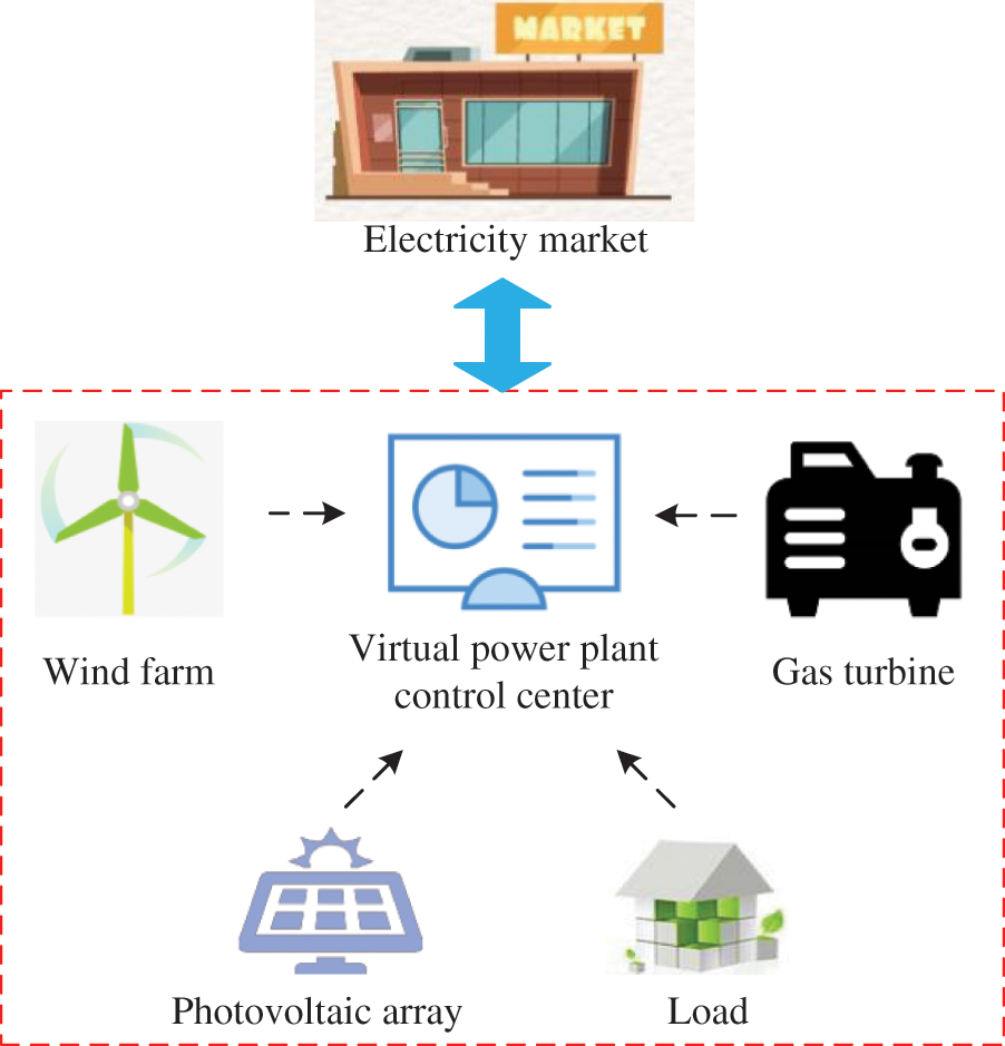
Figure 1: Schematic of studied virtual power plant
The distributionally robust formulation of virtual power plants corresponds to a two-stage optimization problem, in which the gas turbine unit commitment decisions and day-ahead bidding strategy in electricity markets are the first-stage decision variables. These decision variables should be decided one day ahead when the renewable power output is unknown. Other dispatch variables (including the gas turbine power output and power system dispatch decisions) are the second-stage decision variables, which are decided after renewable power output is realized. The objective function of the first stage model is expressed as:
where t represents dispatch periods; e represents gas turbines;
where
The power generation cost function of gas turbines is commonly a quadratic function, which can be linearized by the piecewise linearization method [20] as follows:
where m is the number of pieces; be,m and ke,m are the parameters of the linear function.
The first-stage objective function (5) consists of two parts. The first is the gas turbine unit commitment costs minus the virtual power plant revenue in the electricity market, while the second part is the expected value of the power generation cost of gas turbines calculated by Eq. (6) under the worst probability distribution of the renewable power output.
The constraints of the first stage model state the relationship of binary variables of gas turbines:
where tU and tD stand for the minimum start-up and shut-down time of gas turbine e, respectively.
Eq. (8) is the logical constraint of binary variables, while Eqs. (9) and (10) refer to the minimum start-up and shut-down time constraints of gas turbines.
The second-stage constraints include the gas turbine power output constraint and the distribution network constraint. It is worth mentioning that the distribution network constraint is taken into consideration here, in order to avoid power system problems such as bus voltage violation and branch overload.
The power output constraints of gas turbines can be expressed as follows:
where
Eqs. (11) and (12) are the upper and lower limits of the active and reactive power output of gas turbines, while Eqs. (13) and (14) stand for the ramp-up and ramp-down constraints of gas turbines.
The distribution network constraints is be described with the linearized DistFlow branch model [21]:
where w represents renewable energy units; i, j, and l stand for buses;
Eqs. (15) and (16) indicate active power balance constraints. Eq. (17) represents reactive power balance constraint. Eq. (18) refers to the relation between nodal voltage magnitudes and branch power flows. Eqs. (19)–(21) stand for the upper and lower limits for active branch power flow, reactive branch power flow, and bus voltage magnitudes.
The distributionally robust optimization model is a typical NP-hard problem, for which the optimal solution of the second-stage decision variables cannot be found until traversing all realizations of uncertain parameters. The affine policy can effectively overcome this computational obstacle. Under the policy, the second-stage decision variables affinely depend on uncertain parameters. In order to match with the extended ambiguity set G, the decision variable y in the second stage is constrained to be an affine function of the uncertain variable w and the auxiliary variable v, which is expressed as follows:
where y0, Yw, and Yv are linear coefficients of the affine function, representing the decision variables.
Taking
The linear affine functions of other second-stage decision variables (including
For notational brevity, the day-ahead distributionally robust optimization model of virtual power plants is represented as the following matrix/vector form:
with
where A, E, G, M, b, c, d, and h are coefficient matrices and vectors of the optimization model.
Eqs. (24) and (25) are the matrix/vector forms of the objective function and constraints in the first stage, respectively; Eqs. (26) and (27) are the matrix/vector forms of the objective function and constraints in the second stage, respectively. It should be noted that in Eq. (24), the ambiguity set F has been replaced by the extended ambiguity set G.
The supremum (sup) problem in the objective function (24), which is an infinite-dimensional problem, is difficult to solve. To deal with this, we first express the supremum problem as the following semi-infinite optimization problem, according to the definition of the extended ambiguity set G(3):
where f(w, v) is the joint probability density function of w and v; α, β, and γ are dual variables of the constraint Eqs. (29)–(31), respectively.
Eqs. (29)–(31) correspond to the formulas in the first to third lines in the ambiguity set G(3); Eq. (32) highlights the non-negativity of f(w, v).
Then, the strong duality theory is applied to transform the semi-infinite optimization problem (28)–(32) to a finite-dimensional dual problem. Replacing the supremum problem in the original problem (24)–(27) with the obtained finite-dimensional dual problem, we can have the equivalent form of the original problem as follows:
Finally, the second-order cone duality theory is used to convert the robust constraints (36) and (37) into their dual problems (see Appendix A for detailed conversion processes), and the final form of the distributionally robust optimization model can be expressed as follows:
where δ, ε, η, κ, π, ρ are the dual variables deriving from the dual transformation of robust constraint (36); 1 is the vector with all elements being 1; (
In this way, the original distributionally robust optimization model (24)–(27) can be equivalently transformed into the deterministic mixed-integer second-order cone programming problem (38)–(50).
A virtual power plant composed of three gas turbines, one wind farm, one photovoltaic array, and loads in the distribution network is tested here. The parameters of gas turbines are shown in Table B1, Appendix B. The wind farm is assumed to include two 1.5-MW wind turbines (Goldwind GW 77/1500 [22]), whose cut-in, cut-out, and rated wind speeds are 3, 22, and 11 m/s, respectively, and fitting coefficients are a0 = 0.50, a1 = −0.31, a2 = 0.059, a3 = −0.0025. The photoelectric transformation efficiency of the photovoltaic array is 15.7% [23] and the total surface area of the photovoltaic array is 25000 m2. Historical data of wind speed and solar irradiance for Jan. 2021 [24] are used to calculate expected values of wind and photovoltaic power output (see Appendix C for detailed calculation processes). The expected values of wind power output, photovoltaic power output, and loads are shown in Fig. B1, Appendix B. The IEEE 33-bus distribution system is considered here and its structure is shown in Fig. 2. The three gas turbines, wind farm, and photovoltaic array are located at nodes 22, 18, 33, 12, and 25, respectively. The parameters of the IEEE 33-bus system can be found in [25]. The electricity market price [26] is shown in Fig. B2, Appendix B. The commercial solver MOSEK in the GAMS platform is used to solve finally mixed-integer second-order cone programming problem, with the relative gap set to 0.1%.
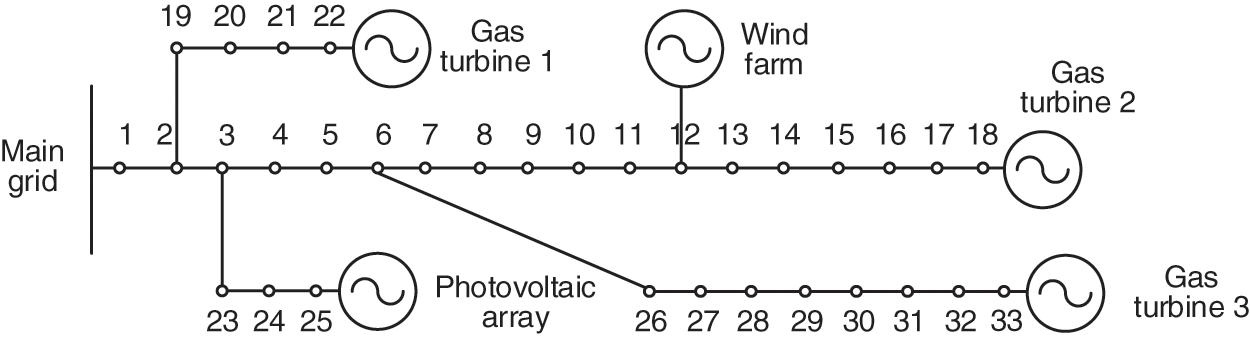
Figure 2: IEEE 33-bus distribution test system
4.2 Comparison with Different Optimization Approaches
1) Optimization results
The proposed distributionally robust optimization approach is compared with the stochastic optimization and traditional robust optimization approaches. The relative standard deviation (obtained by
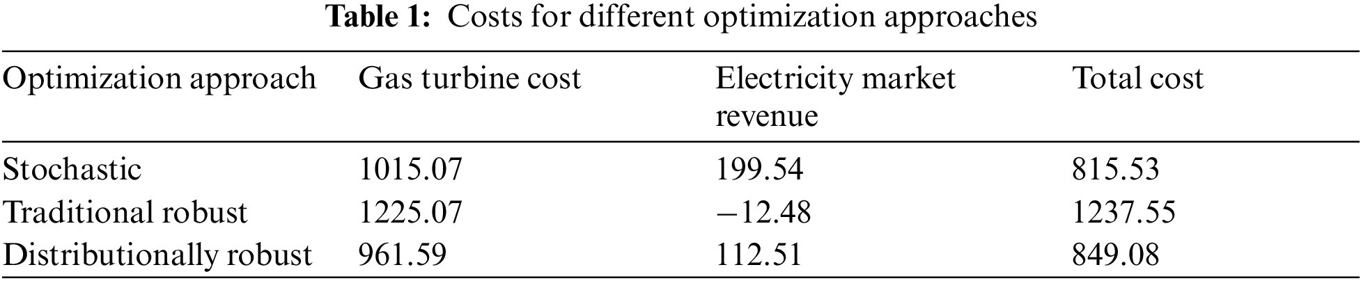
The traded energy (sold if positive or purchased if negative) of the virtual power plant in electricity markets and costs for the three optimization approaches are shown in Fig. 3 and Table 1, respectively.
The stochastic, traditional robust, and distributionally robust optimization approaches focus on the expected distribution, the worst-case distribution, and the worst-case of uncertainties, respectively. As such, the decisions of the stochastic optimization approach are most radical among these three methods, expressed as the virtual power plant tends to sell more energy and purchase less energy in electricity markets, which can be observed in Fig. 3. Such a strategy can obtain a lower total cost under ideal conditions where probability distributions of renewable power output are estimated precisely (see Table 1). However, less energy purchased may bring serious load shedding problems to the virtual power plant under a few unforeseen scenarios with low renewable power output (detailed analyses can be found below). The traditional robust optimization approach, in contrast, is the most conservative method, in which the virtual power plant tends to sell less energy and purchase more energy. This conservative strategy yields a relatively high total cost. The distributionally robust optimization approach can mitigate the over-conservative problem of the traditional one by further capturing the distribution information of renewable power output, which finally reduces the total cost of the virtual power plant by 31.39%.
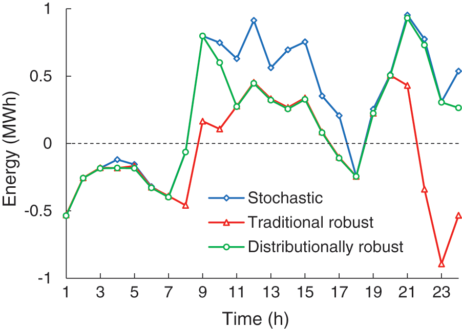
Figure 3: Traded energy for different optimization approaches
We further test the performance of stochastic, traditional robust, and distributionally robust optimization approaches by out-of-sample analyses. In order to do this, we first solve the three models to obtain the first-stage decision variables (i.e., the gas turbine unit commitment decisions and day-ahead bidding strategy), and then solve the second-stage model for the given first-stage decision variables under 500 out-of-sample scenarios. Note that the solution results of the stochastic optimization approach in Table 1 are obtained under the predetermined distribution (i.e., the Gaussian distribution). However, the actual probability distribution is normally different from the predetermined distribution because of estimation or forecast errors. In this regard, load shedding may emerge in the virtual power plant when a few unforeseen scenarios occur in practice. For ensuring the solvability under all out-of-sample scenarios, we further add a load shedding variable in the power balance constraint (15), and the product of the load shedding variable and a penalty cost (4000 $/MWh [28]) in the objective function (5).
The expected load shedding and total cost for the three approaches under a discrepant distribution (uniform distribution as a comparative example) are listed in Table 2. We can see that the stochastic optimization method suffers serious load shedding problems in this case with inaccurate estimations of probability distributions. This problem, however, is effectively avoided in the distributionally robust optimization approach, because descriptive statistics instead of detailed probability distributions are employed to cover the vagueness of the distribution information in this approach.
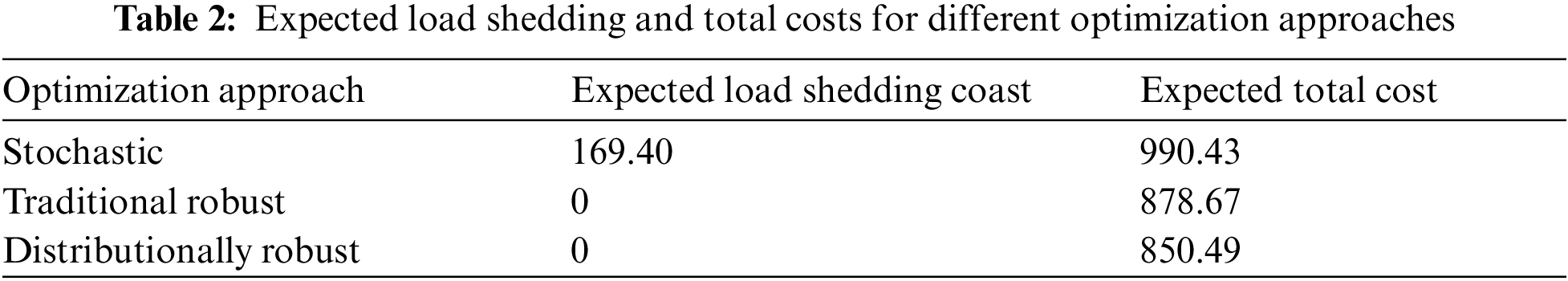
Generally, the distributionally robust optimization approach is the intermediation of the stochastic and traditional robust approach, which can guarantee a relatively low total cost and prevent serious load shedding simultaneously. That is, the distributionally robust optimization approach represents a good trade-off between robustness and economy, and thus should be favored by virtual power plant operators.
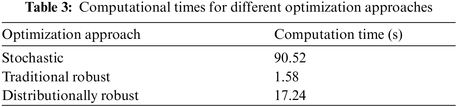
2) Computational times
The computational times for stochastic optimization, robust optimization, and distributionally robust optimization models are shown in Table 3. The stochastic optimization approach suffers from a large computational burden because of scenario enumerations. By comparison, the calculation time of the distributionally robust optimization approach is reduced by 80.95%, since heavy calculations arising from scenario enumerations are avoided. Besides, the computational time of the distributionally robust optimization model is less than 20 s, which is much less than the time threshold of the day-ahead dispatch problem. This is because the proposed solution method converts the complex distributionally optimization model into a deterministic mixed-integer second-order cone programming problem, and thereby greatly reducing the difficulty of model solving. This verifies the effectiveness of the proposed solution method.
The moment information of renewable power output is incorporated in the ambiguity set to depict its probability distribution features. This section explores the impact of the moment information on the optimization results. Here, the relative standard deviation is used to reflect the change of the variance. The total traded energy in the electricity market and the objective function value (total cost) of the virtual power plant as shown in Fig. 4, after solving the robust optimization model under different relative standard deviations.
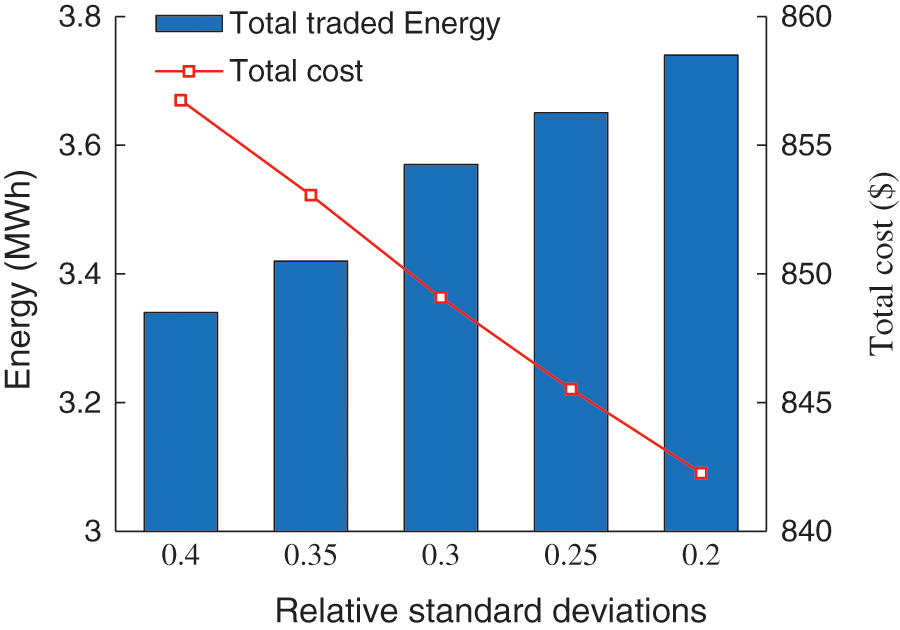
Figure 4: Traded energy and objective functions with different relative standard deviations
The traded energy of the virtual power plant in the electricity market gradually increases with the decreasing relative standard deviation. This is because the decreasing of the relative standard deviation means that the decreased fluctuation of the renewable power output. In this regard, the virtual power plant only needs to buy less energy (or sell more energy) in electricity markets to cope with the risks caused by the fluctuation of renewable power output, which reduces the total cost of the virtual power plant. This means that the adaptability of the dispatch strategy to the fluctuation of renewable power output is improved in the distributionally robust optimization approach. That is, the distributionally robust optimization approach enables the operator to adjust the dispatch strategy based on the moment information of the renewable power output so as to reduce the total cost. This adjustment capability cannot be achieved in the traditional robust optimization approach.
In this study, we consider the impact of the uncertainty of renewable power output on virtual power plant dispatch, and propose a day-ahead distributionally robust optimization dispatch model for the virtual power plant. The solution results show that:
1) Compared with stochastic and traditional robust optimization methods, the proposed distributionally robust optimization method can better balance the robustness and economy of dispatch decisions.
2) The proposed distributionally robust optimization approach can adjust the dispatch strategy of the virtual power plant according to the moment information of the renewable power output, and thus the total cost of the virtual power plant is reduced.
3) The solve difficulty of the distributionally robust optimization model is effectively reduced by the proposed solution method, which results in that the proposed model can be solved in a short time.
Funding Statement: This work was supported by the Technology Project of State Grid Jiangsu Electric Power Co., Ltd., China, under Grant J2020090.
Conflicts of Interest: The authors declare that they have no conflicts of interest to report regarding the present study.
References
1. Naval, N., Yusta, J. M. (2021). Virtual power plant models and electricity markets–A review. Renewable & Sustainable Energy Reviews, 149, 1–13. DOI 10.1016/j.rser.2021.111393. [Google Scholar] [CrossRef]
2. Nosratabadi, S. M., Hooshmand, R. A., Gholipour, E. (2017). A comprehensive review on microgrid and virtual power plant concepts employed for distributed energy resources scheduling in power systems. Renewable & Sustainable Energy Reviews, 67, 341–363. DOI 10.1016/j.rser.2016.09.025. [Google Scholar] [CrossRef]
3. Zhou, Y., Wei, Z., Sun, G., Cheung, K. W., Zang, H. et al. (2019). Four-level robust model for a virtual power plant in energy and reserve markets. IET Generation, Transmission & Distribution, 13(11), 2036–2043. DOI 10.1049/iet-gtd.2018.5197. [Google Scholar] [CrossRef]
4. Yi, Z., Xu, Y., Wang, H., Sang, L. (2021). Coordinated operation strategy for a virtual power plant with multiple DER aggregators. IEEE Transactions on Sustainable Energy, 12(4), 2445–2458. DOI 10.1109/TSTE.2021.3100088. [Google Scholar] [CrossRef]
5. Rahimia, M., Ardakania, F. Z., Ardakanib, A. J. (2021). Optimal stochastic scheduling of electrical and thermal renewable and non-renewable resources in virtual power plant. International Journal of Electrical Power & Energy Systems, 127, 1–19. DOI 10.1016/j.ijepes.2020.106658. [Google Scholar] [CrossRef]
6. Kardakos, E. G., Simoglou, C. K., Bakirtzis, A. G. (2016). Optimal offering strategy of a virtual power plant: A stochastic bi-level approach. IEEE Transactions on Smart Grid, 7(2), 794–806. DOI 10.1109/TSG.2015.2419714. [Google Scholar] [CrossRef]
7. Shabanzadeh, M., Sheikh-El-Eslami, M. K., Haghifam, M. R. (2017). Risk-based medium-term trading strategy for a virtual power plant with first-order stochastic dominance constraints. IET Generation, Transmission & Distribution, 11(2), 520–529. DOI 10.1049/iet-gtd.2016.1072. [Google Scholar] [CrossRef]
8. Naughton, J., Wang, H., Cantoni, M., Mancarella, P. (2021). Co-optimizing virtual power plant services under uncertainty: A robust scheduling and receding horizon dispatch approach. IEEE Transactions on Power Systems, 36(5), 3960–3972. DOI 10.1109/TPWRS.2021.3062582. [Google Scholar] [CrossRef]
9. Baringo, A., Baringo, L., Arroyo, M. (2019). Day-ahead self-scheduling of a virtual power plant in energy and reserve electricity markets under uncertainty. IEEE Transactions on Power Systems, 34(3), 1881–1894. DOI 10.1109/TPWRS.59. [Google Scholar] [CrossRef]
10. Bertsimas, D., Sim, M., Zhang, M. (2018). Adaptive distributionally robust optimization. Management Science, 65(2), 1–30. DOI 10.1287/mnsc.2017.2952. [Google Scholar] [CrossRef]
11. Delage, E., Ye, Y. (2010). Distributionally robust optimization under moment uncertainty with application to data-driven problems. Operations Research, 58(3), 595–612. DOI 10.1287/opre.1090.0741. [Google Scholar] [CrossRef]
12. Wiesemann, W., Kuhn, D., Sim, M. (2014). Distributionally robust convex optimization. Operations Research, 62(6), 1358–1376. DOI 10.1287/opre.2014.1314. [Google Scholar] [CrossRef]
13. Xiong, P., Jirutitijaroen, P., Singh, C. (2017). A distributionally robust optimization model for unit commitment considering uncertain wind power generation. IEEE Transactions on Power Systems, 32(1), 39–49. DOI 10.1109/TPWRS.2016.2544795. [Google Scholar] [CrossRef]
14. Zhang, Y., Shen, S., Mathieu, J. L. (2017). Distributionally robust chance-constrained optimal power flow with uncertain renewables and uncertain reserves provided by loads. IEEE Transactions on Power Systems, 32(2), 1378–1388. DOI 10.1109/TPWRS.2016.2572104. [Google Scholar] [CrossRef]
15. Wei, W., Liu, F., Mei, S. (2016). Distributionally robust co-optimization of energy and reserve dispatch. IEEE Transactions on Sustainable Energy, 7(1), 289–300. DOI 10.1109/TSTE.2015.2494010. [Google Scholar] [CrossRef]
16. Zhou, Y., Shahidehpour, M., Wei, Z., Li, Z., Sun, G. et al. (2020). Distributionally robust unit commitment in coordinated electricity and district heating networks. IEEE Transactions on Power Systems, 35(3), 2155–2166. DOI 10.1109/TPWRS.59. [Google Scholar] [CrossRef]
17. Zheng, X., Qu, K., Lv, J., Li, Z., Zeng, B. (2021). Addressing the conditional and correlated wind power forecast errors in unit commitment by distributionally robust optimization. IEEE Transactions on Sustainable Energy, 12(2), 944–954. DOI 10.1109/TSTE.2020.3026370. [Google Scholar] [CrossRef]
18. Liu, L., Hu, Z., Duan, X., Pathak, N. (2021). Data-driven distributionally robust optimization for real-time economic dispatch considering secondary frequency regulation cost. IEEE Transactions on Power Systems, 36(5), 4172–4184. DOI 10.1109/TPWRS.2021.3056390. [Google Scholar] [CrossRef]
19. Pourahmadi, F., Kazempour, J. (2021). Distributionally robust generation expansion planning with unimodality and risk constraints. IEEE Transactions on Power Systems, 36(5), 4281–4295. DOI 10.1109/TPWRS.2021.3057265. [Google Scholar] [CrossRef]
20. Zhao, C., Guang, Y. (2013). Unified stochastic and robust unit commitment. IEEE Transactions on Power Systems, 28(3), 3353–3361. DOI 10.1109/TPWRS.59. [Google Scholar] [CrossRef]
21. Yeh, H., Gayme, D. F., Low, S. H. (2012). Adaptive VAR control for distribution circuits with photovoltaic generators. IEEE Transactions on Power Systems, 27(3), 1656–1663. DOI 10.1109/TPWRS.2012.2183151. [Google Scholar] [CrossRef]
22. Goldwind GW 77/1500 (2021). https://en.wind-turbine-models.com/turbines/106-goldwind-gw-77-1500. [Google Scholar]
23. Yang, H., Xiong, T., Qiu, J., Qiu, D., Dong, Z. Y. (2016). Optimal operation of DES/CCHP based regional multi-energy prosumer with demand response. Applied Energy, 167, 353–565. DOI 10.1016/j.apenergy.2015.11.022. [Google Scholar] [CrossRef]
24. NREL Flatirons Campus (M2) (2021). https://midcdmz.nrel.gov/apps/sitehome.pl?site=NWTC#. [Google Scholar]
25. Baran, M. E., Wu, F. F. (1989). Network reconfiguration in distribution systems for loss reduction and load balancing. IEEE Transactions on Power Systems, 4(2), 1401–1407. DOI 10.1109/61.25627. [Google Scholar] [CrossRef]
26. PJM-Markets & Operations (2021). http://www.pjm.com/markets-and-operations.aspx. [Google Scholar]
27. Hong, Y. Y., Satriani, T. R. A. (2020). Day-ahead spatiotemporal wind speed forecasting using robust design-based deep learning neural network. Energy, 209, 1–13. DOI 10.1016/j.energy.2020.118441. [Google Scholar] [CrossRef]
28. Zamani, A. G., Zakariazadeh, A., Jadid, S. (2016). Day-ahead resource scheduling of a renewable energy based virtual power plant. Applied Energy, 169, 324–340. DOI 10.1016/j.apenergy.2016.02.011. [Google Scholar] [CrossRef]
This appendix provides the transformation from robust constraint (36) to (41)–(45). Robust constraints (37) can also be transformed into (46)–(50) by a similar process. Put affine function (22) into robust constraint (36), we obtain:
Then, (A1) is rewritten into the following equation under the worst scenario:
In (A2), the uncertain variable w and auxiliary variable v are within the constraints of the extended uncertainty set
Introduce the auxiliary variables τ, ψ, ζ into the set
where δ, ε, η, κ, π, θ, ρ are the dual variables of the corresponding constraint formula; 1 means a vector with all elements being 1.
It is worth mentioning that the constraint Eqs. (A6)–(A9) collectively represent the constraint Eq. (A3), i.e., (w
Eq. (A2) satisfies the constraints (A4)–(A10). Thus, (A2) can be transformed into the following dual problem using the second-order cone duality theory:
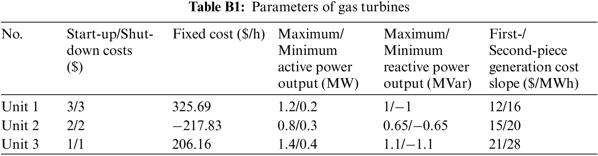
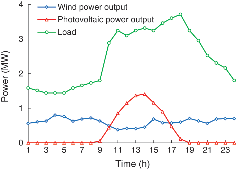
Figure B1: Expected values of wind power output, photovoltaic power output, and loads
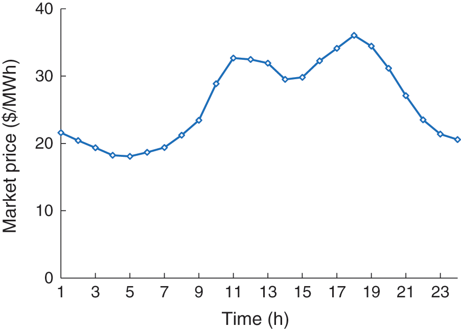
Figure B2: Electricity market prices
This appendix provides the calculation steps of expected values of wind and photovoltaic power output, which are illustrated as follows:
Step 1: Expected values of wind speed and solar irradiance are calculated by their historical data for January 2021.
Step 2: Wind power output is calculated by wind speed according to the wind power conversion curve:
where
Step 3: Photovoltaic power output is calculated by the solar irradiance-power conversion function:
where
This appendix provides the illustrations and steps of the scenario reduction method. Note that scenarios of renewable power output generated by the Monte Carlo method are very huge, which brings an expensive computational burden for solving the stochastic optimization model. Thus, it is essential to obtain a subset of renewable power output scenarios with a limited number of scenarios and without losing the generality of the original set. The scenario reduction method is such an effective method that can reduce the scenario number and maximally retain the fitting accuracy of samples.
Assume that the number of renewable power output scenarios generated by the Monte Carlo method is N, with 1/N probability of each scenario (i.e., ps = 1/N). The steps of the scenario reduction method are detailed as follows:
Step 1: Set an objective number of scenarios n, and specify the initial number of reduced scenarios n* = N.
Step 2: Calculate the Kantorovich distance D between each pair of scenarios (si, sj), where D is the absolute value of power output difference between scenarios si and sj, i.e.,
Step 3: For each scenario sk, select the scenario sl with the minimum distance
Step 4: Select and delete the scenario o with minimum
Step 5: If n* = n, present reduced scenarios and their probabilities; otherwise, reorder scenarios and return to Step 2.
 | This work is licensed under a Creative Commons Attribution 4.0 International License, which permits unrestricted use, distribution, and reproduction in any medium, provided the original work is properly cited. |