Energy Engineering

---

DOI: 10.32604/ee.2022.020344

ARTICLE

T-Shaped Transmission Line Fault Location Based on Phase-Angle Jump Checking

Jia’an Xie1,*, Yurong Wang2, Guobin Jin3 and Mucheng Wu1

1Foshan Power Supply Bureau, Guangdong Power Grid Co., Ltd., Foshan, 528000, China
2School of Electrical Engineering, Southeast University, Nanjing, 210018, China
3School of Electrical Engineering, Northeast Electric Power University, Jilin, 132012, China
*Corresponding Author: Jia’an Xie. Email: xiejiaan006666@163.com
Received: 17 November 2021; Accepted: 08 April 2022

1  Introduction

T-shaped transmission line has the characteristics of flexible operation mode, large transmission capacity and good economy, so it is widely used in power systems. Due to the more complex connection mode, more connection points and wider influence range of T-shaped transmission line, so when the T-shaped transmission line fault occurs, the realization of fast and high-precision fault location can effectively improve the efficiency of manual line inspection, and then shorten the outage time of transmission line, which has great practical significance to improve the safety, reliability and stability of power systems.

1.1 Related Research Works

In recent years, scholars have conducted a lot of research on fault location methods for T-shaped transmission line, which can be divided into two categories from the principle of fault location: traveling wave location method and fault analysis location method. The principle of the first type of traveling wave location method is simple. The fault location is realized by capturing the time difference of the fault traveling wave heads at 3-terminal of T-shaped transmission line. However, due to the difficulty in accurately capturing fault traveling wave heads, the fault location accuracy cannot be guaranteed, and the high hardware requirements and large investment scale limit its application scale [1–4].

The second type of fault analysis and location methods can be divided into synchronous fault analysis method [5–13] and asynchronous fault analysis method [14–24] according to the synchronization and asynchrony of 3-terminal measurement data. The literature [11–13] achieved the purpose of fault location by constructing a phase-comparison function based on the synchronous measurement of phasors at the 3-terminal of the T-shaped transmission line, but the existing phase comparison function method basically realizes the fault point location by segmented and point-by-point search and the accuracy of fault location is mainly determined by the search step-size. The setting of search step-size is too large, the search times and the amount of calculation are small, but the location accuracy is low; The setting of search step-size is too small and the fault location accuracy is high, but the search times and calculation will increase greatly. Therefore, the existing phase comparison fault location method cannot effectively solve the contradiction between accuracy and calculation. Literature [14,15] deduced the asynchronous fault location algorithm of T-shaped transmission line by using centralized parameter model, since the influence of distributed parameter characteristics is not considered, its fault location accuracy is low in high-voltage and long-distance T-shaped transmission line, while literature [16] deduced the asynchronous fault location equation suitable for T-shaped transmission line by using distributed parameter model, but the calculation results have the problem of coexistence of real root and virtual root, complex discrimination calculation of real root and virtual root is needed to determine the actual fault distance, which is not conducive to the rapid calculation requirement of fault location. Moreover, the asynchronous fault location method of T-shaped transmission line proposed in literature [14–16] has the problem of location dead zone near T-node, which limits its applicability.

1.2 Research Contribution

In this paper, a new fault location algorithm for T-shaped transmission line based on phase angle jump checking is proposed, which can realize the purpose of rapid selection of fault branch and high-precision fault location. The simulation results show the feasibility and effectiveness of the algorithm, and the algorithm has the characteristics of strong versatility, high fault location accuracy, immunity to transition resistance, and has the prospect of practical application. The main contributions of this manuscript are summarized below:

•   The distance function method for fast identification of fault branch is proposed. By calculating the phase-angle of distance function value of each branch and judging whether its symbol is negative, the fault branch can be determined quickly.

•   The high-precision fault location algorithm is proposed and the calculation equation is derived. Using the equation, all roots (including real root and virtual roots) can be calculated.

•   There is no factor of Rf in the fault location equation, so the fault location result is not affected by the transition resistance in principle.

•   The phase angle jump check function is proposed. The real root and virtual roots are respectively substituted into the phase angle jump check function for calculation. By judging whether the value is negative, the only real root can be quickly determined, which is the fault distance.

1.3 Organization of Contents

The paper is organized into six sections. The Section 1 describes the review of literature, research gaps, and contribution of this manuscript. The high-precision fault location equation for 2-terminal transmission lines is described in the Section 2. All the steps of the proposed algorithm for fault branch selection and fault location are detailed in the Section 3. The technical flow chart for implementing the fault location algorithm is described in Section 4. Performance estimation of the algorithm is illustrated in Section 5. A comparative study of this proposed algorithm with the algorithm reported in the literature is also included in this section, as well as a correlation study of the capacitance parameter error and the fault location error. Finally, research is concluded in Section 6 of the manuscript.

2  Analysis of 2-Terminal High Precision Fault Location Model

Fig. 1 shows the positive sequence equivalent network when a short-circuit fault occurs in 2-terminal transmission line. The total length of the line mn is L, where point f is the fault point, point k is the reference point, and point k is located to the right of point f. According to Fig. 1, the distribution of fundamental positive sequence voltage and current phasors at points f and k away from the point m can be obtained [8,9].

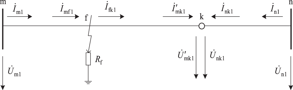
Figure 1: Fault diagram of transmission line

{U˙f1=U˙m1cosh(γ1lmf)−Zc1I˙m1sinh(γ1lmf)I˙mf1=I˙m1cosh(γ1lmf)−U˙m1Zc1sinh(γ1lmf)(1)

{U˙′mk1=U˙nk1I˙fk1=I˙mf1−I˙f1(2)

U˙′mk1=U˙f1cosh(γ1lfk)−Zc1I˙fk1sinh(γ1lfk)(3)

I˙′mk1=I˙fk1cosh(γ1lfk)−U˙f1Zc1sinh⁡(γ1lfk)(4)

In Eqs. (1)−(4): U˙f1 and I˙mf1 are the fundamental positive sequence voltage phasor and current phasor at fault point f estimated by the electric quantities of point m; U˙′mk1, I′˙mk1 and U˙nk1, I˙nk1 respectively are the fundamental positive sequence voltage phasor and current phasor at point k estimated by the electric quantities of point m and point n; I˙f1 is the fundamental positive sequence current phasor injected into fault point f; U˙m1 and I˙m1 are the fundamental positive sequence voltage phasor and current phasor at point m; lmf is the distance from point m to f, and lfk is the distance from point f to k; γ1=(R0+jw1L0)(G0+jw1C0) and Zc1=(R0+jw1L0)/(G0+jw1C0) are respectively called the fundamental positive sequence propagation constant and fundamental positive sequence characteristic impedance; L0 is the line inductance value per unit length, C0 is the line capacitance value per unit length, and w1 is the fundamental wave angular frequency.

Then Eq. (5) can be obtained by combining Eqs. (1)−(3).

U˙mk1−U˙nk1=Zc1I˙f1sinh[γ1(lmf−lmk)](5)

Eq. (6) can be obtained by combining Eqs. (1), (2) and (4).

I˙mk1+I˙nk1=I˙f1sinh⁡[γ1(lmf−lmk)](6)

In Eqs. (5) and (6): U˙mk1=U˙m1cosh⁡(γ1lmk)−Zc1I˙m1sinh⁡(γ1lmk), U˙nk1=U˙n1cosh⁡(γ1(L−lnk))−Zc1I˙n1sinh⁡(γ1(L−lnk)), I˙mk1=I˙m1cosh⁡(γ1lmk)−U˙m1sinh⁡(γ1lmk)/Zc1, I˙nk1=I˙n1cosh⁡(γ1(L−lmk))−U˙n1sinh⁡(γ1(L−lmk))/Zc1.

It can be seen from Eq. (5) that when lmf−lmk=0, the condition of Zc1I˙f1sinh⁡[γ1(lmf−lmk)]=0 must be valid, that is, U˙mk1=U˙nk1 must be valid at the fault point. At the same time, if lmf−lmk≠0, the condition of Zc1I˙f1sinh⁡[γ1(lmf−lmk)]=0 may also be valid, that is, U˙mk1=U˙nk1 may be valid at the non-fault point.

Based on above analysis, Eq. (7) can be constructed for fault location calculation.

{U˙m1(lmf)=A1cosh(γ1lmf)−A2sinh(γ1lmf)U˙n1(L−lmf)=A3coshγ1(L−lmf)−A4sinhγ1(L−lmf)U˙m1(lmf)=U˙n1(L−lmf)(7)

In Eq. (7): A1=U˙m1, A2=Zc1I˙m1, A3=U˙n1, A4=Zc1I˙n1, L is the line length, lmf is the fault distance. Then Eq. (8) can be obtained from Eq. (7).

lmf=12γ1ln⁡[(A3−A4)eγ1L−(A1+A2)][(A1−A2)−(A3+A4)e−γ1L](8)

Based on above analysis, multiple roots (including real root and virtual roots) may be obtained in Eq. (8), and the only real root must be determined by accurate identification to achieve the purpose of fault location.

Therefore, a new criterion method based on phase angle jump checking is constructed, which can achieve the purpose of accurate fault location. Simultaneous Eqs. (5) and (6), and considering the asynchronous phase angle difference of PMU systems at point m and point n is δ, the function f(lmk) can be constructed, as shown in Eq. (9).

f(lmk)=U˙mk1−ejδU˙nk1I˙mk1+ejδI˙nk1=Zc1tanh[γ1(lmf−lmk)](9)

Set lmk−lmf=Δl, lmk=lmf−Δl, then Eq. (9) can be transformed into Eq. (10).

f(lmf−Δl)=U˙m1(lmf−Δl)−ejδU˙n1[ L−(lmf−Δl) ]I˙m1(lmf−Δl)+ejδI˙n1[ L−(lmf−Δl) ]     =Zc1tanh(γ1Δl)(10)

In Eqs. (9) and (10): L is the line length, U˙m1(lmf−Δl) and I˙m1(lmf−Δl) are the fundamental positive sequence voltage phasor and current phasor at the distance from point m to lmf−Δl; U˙n1[L−(lmf−Δl)] and I˙n1[L−(lmf−Δl)] are the fundamental positive sequence voltage phasor and current phasor at the distance from point n to L−(lmf−Δl), δ is the asynchronous phase angle, which can be calculated from Eq. (11).

δ=arg⁡(U˙mn1)−arg⁡(U˙n1)(11)

In Eq. (11): U˙mn1 is the fundamental positive sequence voltage phasor at point n calculated by the electric quantities of point m and U˙n1 is the fundamental positive sequence voltage phasor extracted by the electric quantity of point n before the fault occurs.

From Eq. (10), when Δl>0, arg⁡[f(lmf−Δl)]≈90o; when Δl<0, arg⁡[f(lmf−Δl)]≈−90∘; when Δl=0, arg⁡[f(lmf−Δl)]=0∘, that is, arg⁡[f(lmf−Δl)] will have a jump when crossing from the left to the right of the fault point f.

Based on above analysis, the high-precision fault location equation of 2-terminal synchronous phasor measurement based on distributed parameter model can be derived, as shown in Eq. (12).

{lmf=12γ1ln⁡[(A3−A4)eγ1L−(A1+A2)][(A1−A2)−(A3+A4)e−γ1L]arg⁡[f(lmf−Δl)]⋅arg⁡[f(lmf+Δl)]<0(12)

In Eq. (12): A1=U˙m1, A2=Zc1I˙m1, A3=ejδU˙n1, A4=Zc1ejδI˙n1, L is the line length, lmf is the fault distance, Δl is check step-size.

3  Analysis of Calculation Method for Fault Location of T-Shaped Transmission Line

3.1 Analysis of Fault Branch Selection

A typical T-shaped transmission line is shown in Fig. 2. It is assumed that the phase angle difference between point M and point N is δ1, the phase angle difference between point M and point P is δ2. Then δ1, δ2 can be calculated by Eq. (13).

{δ1=arg⁡(U˙MT1)−arg⁡(U˙NT1)δ2=arg⁡(U˙MT1)−arg⁡(U˙PT1)(13)

In Eq. (13): U˙MT1, U˙NT1, U˙PT1 are the fundamental positive sequence voltage phasors at node T calculated by the electrical quantities of the M, N and P points respectively before the fault occurs.

As shown in Fig. 2, the fault point f is in the branch TN, the voltage and current phasors at node T are taken as U˙T1=(U˙MT1+ejδ2U˙PT1)/2 and I˙T1=I˙MT1+ejδ2I˙PT1, respectively, and then U˙mk1, I˙mk1, U˙nk1, I˙nk1 in Eq. (9) are replaced by U˙NT1, I˙NT1, U˙T1, I˙T1, respectively. At the same time node T is taken as the reference point, then Eq. (14) can be obtained after sorting.

f(lNT)=ejδ1U˙NT1−U˙T1ejδ1I˙NT1+I˙T1=Zc1tanh[γ1(lNf−lNT)](14)

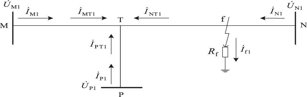
Figure 2: Fault diagram of T-shaped transmission line

According to Eq. (14), since node T is on the left side of the fault point f, that is, lNf−lNT<0, the condition of phase angle arg⁡[f(lNT)]<0 must be valid. If the voltage and current at node T are taken as U˙T1=(ejδ1U˙NT1+ejδ2U˙PT1)/2 and I˙T1=ejδ1I˙NT1+ejδ2I˙PT1, respectively, replace U˙mk1, I˙mk1, U˙nk1, I˙nk1 in Eq. (9) with U˙MT1, I˙MT1, U˙T1, I˙T1, respectively, and use node T as the reference point. Then then Eq. (15) can be obtained after sorting.

f(lMT)=U˙MT1−U˙T1I˙MT1+I˙T1=Zc1tanh(γ1lTf)(15)

According to Eq. (15), the condition that the phase angle arg⁡[f(lMT)]>0 of the non-fault branch MT must be valid. If the voltage and current at node T are taken as U˙T1=(U˙MT1+ejδ1U˙NT1)/2 and I˙T1=I˙MT1+ejδ1I˙NT1, respectively, replace U˙mk1, I˙mk1, U˙nk1, I˙nk1 in Eq. (9) with U˙PT1, I˙PT1, U˙T1, I˙T1, respectively, and use node T as the reference point. Then then Eq. (16) can be obtained after sorting.

f(lPT)=ejδ2U˙PT1−U˙T1ejδ2I˙PT1+I˙T1=Zc1tanh(γ1lTf)(16)

According to Eq. (16), the condition that the phase angle arg⁡[f(lPT)]>0 of the non-fault branch PT must be valid.

From above analysis, by calculating the symbol value of the phase angle function of each branch of T-shaped transmission line (all taking node T as the reference point), the branch where the fault point occurs can be determined, which lays a foundation for the high-precision fault location of T-shaped transmission line proposed in this paper.

3.2 Fault Branch Location Algorithm for T-Shaped Transmission Line

When the fault branch of the T-shaped transmission line is determined (taking NT as the fault branch as an example), use Eq. (17) to perform accurate fault location calculation.

{lNf=12γ1ln⁡[(A3−A4)eγ1L−(A1+A2)][(A1−A2)−(A3+A4)e−γ1L]arg⁡[f(lNf−Δl)]⋅arg⁡[f(lNf+Δl)]<0(17)

In Eq. (17): A1=ejδ1U˙N1, A2=Zc1ejδ1I˙N1, A3=(U˙MT1+ejδ2U˙PT1)/2, A4=I˙MT1+ejδ2I˙PT1, L is the length of fault branch NT, lNf is the fault distance from N side, Δl is check step-size.

3.3 Relative Error Evaluation of Fault Location

The high-precision fault location lNf can be calculated from Eq. (17) to achieve the purpose of high-precision fault location. In order to verify the ranging accuracy of the method in this paper, the relative error index is defined as Eq. (18).

el=|lNf−lfL|×100%(18)

In Eq. (18): lNf is the fault location result, lf is the actual fault distance, and L is the full length of the fault branch.

4  Calculation Steps for Fault Location of T-Shaped Transmission Line

In this paper, a new high-precision fault location method for T-shaped transmission line is proposed, and the flowchart of the technique can be represented by Diagram 1.

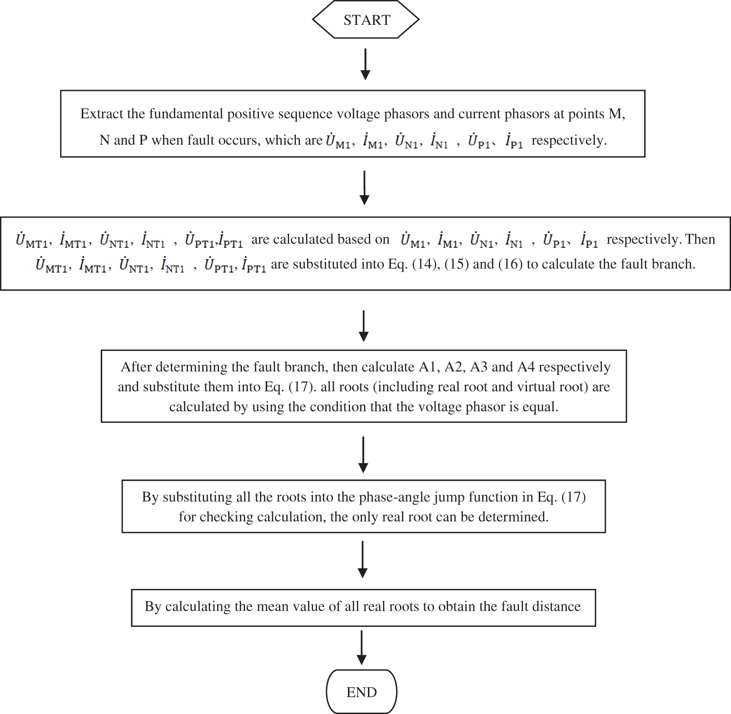
Diagram 1: T-shaped transmission line fault location based on phase-angle jump checking

5  Simulation Calculation

5.1 Simulation Example

The simulation system model of T-shaped transmission line with voltage level of 500 kV, line length of LMT=50km, LPT=70km, LNT=500km is established by using Simulink module in MATLAB software. The fault point is located in the branch NT, and the fault simulation model is shown in Fig. 3.

System parameters on side M: E˙M=1∠10o, ZM1=(0.2534+j2.046)Ω, ZM0=(0.1121+j6.723)Ω.

System parameters on side P: E˙P=1∠15o, ZP1=(0.2534+j2.046)Ω, ZP0=(0.1121+j6.723)Ω.

System parameters on side N: E˙N=1∠0o, ZN1=(2.82+j40.092)Ω, ZN0=(0.224+j12.546)Ω.

Line parameters: L1=0.8858mH/km, R1=0.027Ω/km, C1=0.0127μF/km; L0=2.0671mH/km, R0=0.1948Ω/km, C0=0.009μF/km.

The BC phase to phase short circuit fault occurs in the analog line. The fault point is 70 km away from point N, and the transition resistance is Rf=10Ω. The fault is removed after lasting 68 ms and the data sampling frequency is fs=5000Hz.

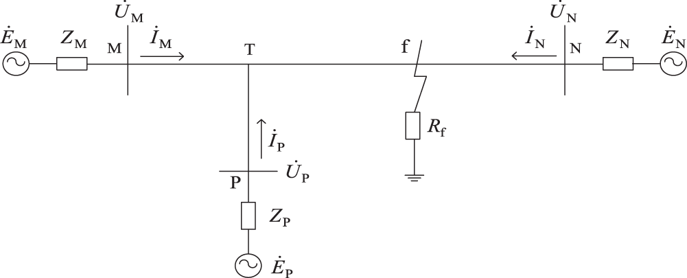
Figure 3: Simulation model of T-shaped transmission line fault

The voltage and current curves of M, N and P points with random noise (SNR=40db) are shown in Fig. 4. A Butter-worth band-pass filter is set in front of the voltage and current synchronous phasor acquisition unit at M, N and P points, the fundamental voltage and current curves extracted by filtering are shown in Fig. 5.

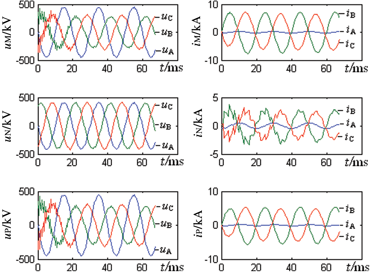
Figure 4: Voltage and current curves of M, N and P points with random noise (SNR=40db)

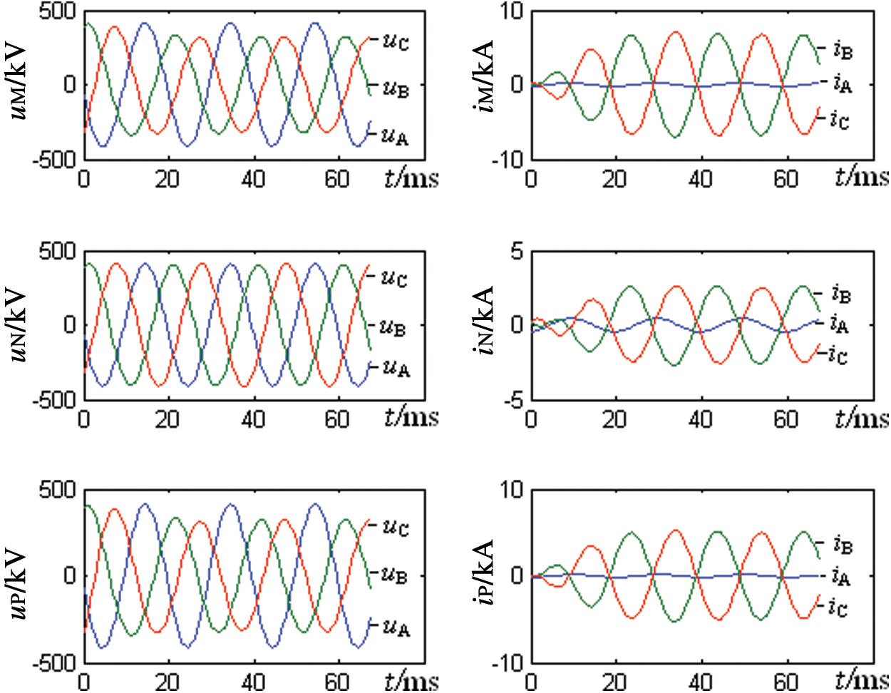
Figure 5: Fundamental voltage and current curves of M, N and P points extracted after butter-worth filtering

So that after the fault occurs in the line, the synchronous phasor acquisition unit can quickly extract the fundamental positive sequence voltage and current phasors, and substitute them into Eq. (17) to calculate the fault distance lNf and verify the step size Δl=0.1km, the results are shown in Fig. 6.

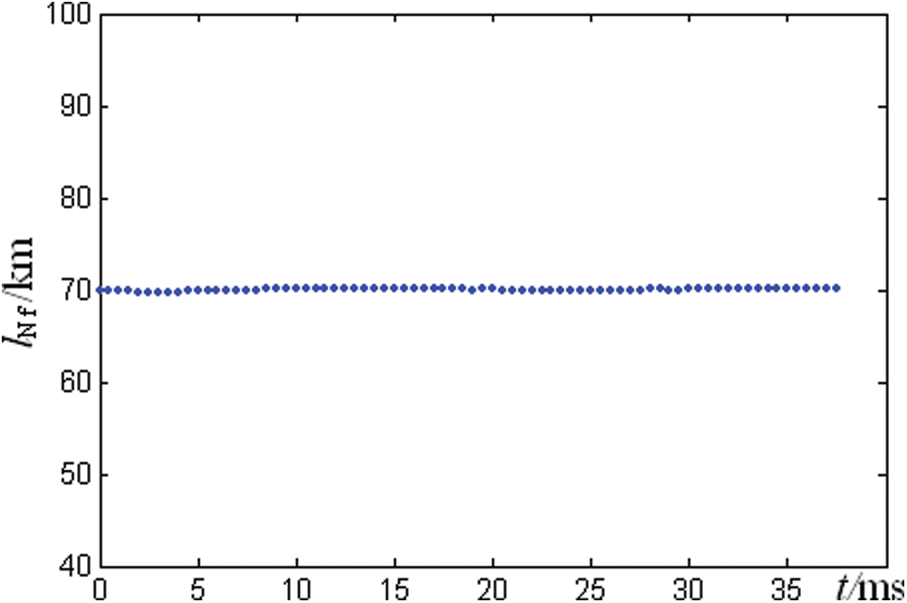
Figure 6: Results of fault location

In order to improve the accuracy of fault location, take the average value of the calculation results shown in Fig. 6, substitute the lNf after taking the average value into the phase angle check function in Eq. (17) for checking, and the final calculation results are shown in Eq. (19).

{lNf=70.0145kmarg⁡[f(70.0145+0.1)]⋅arg⁡[f(70.0145−0.1)]=−2.4540(19)

According to Eq. (19), the fault distance lNf=70.0145km, and the relative error is 0.0029%. From the calculation results, it can be seen that the algorithm has high accuracy.

In order to verify the generality and immunity to the transition resistance of the algorithm, single-phase faults under different transition resistance and different types of faults under the same transition resistance are set for calculation, meanwhile the single-terminal fundamental frequency impedance-based fault location (IBFL) is adopted for comparative study. The results are shown in Tables 1–3, respectively.

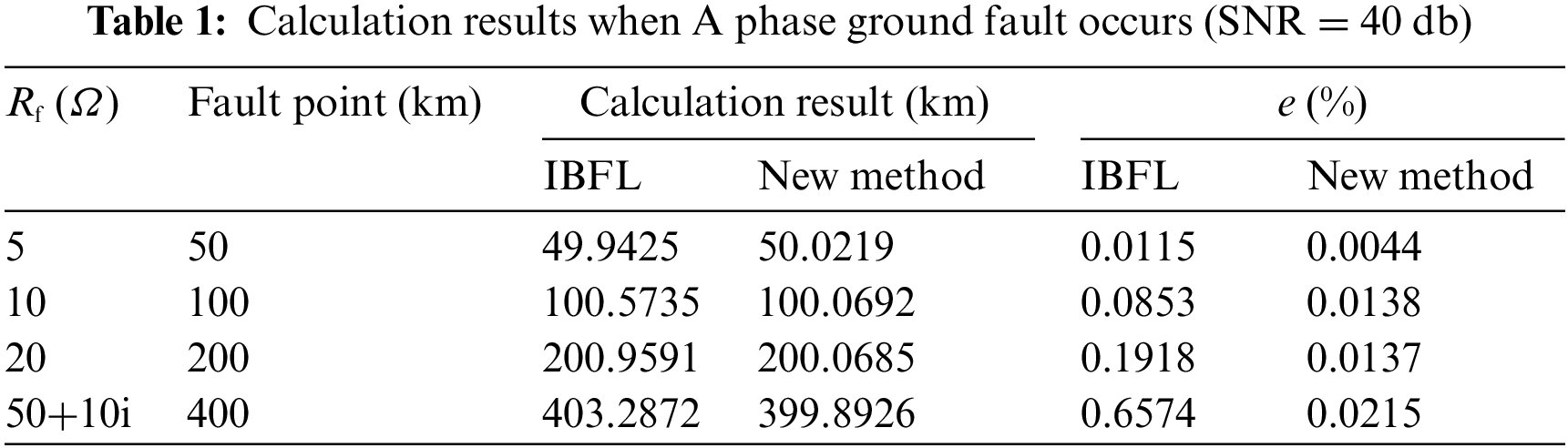
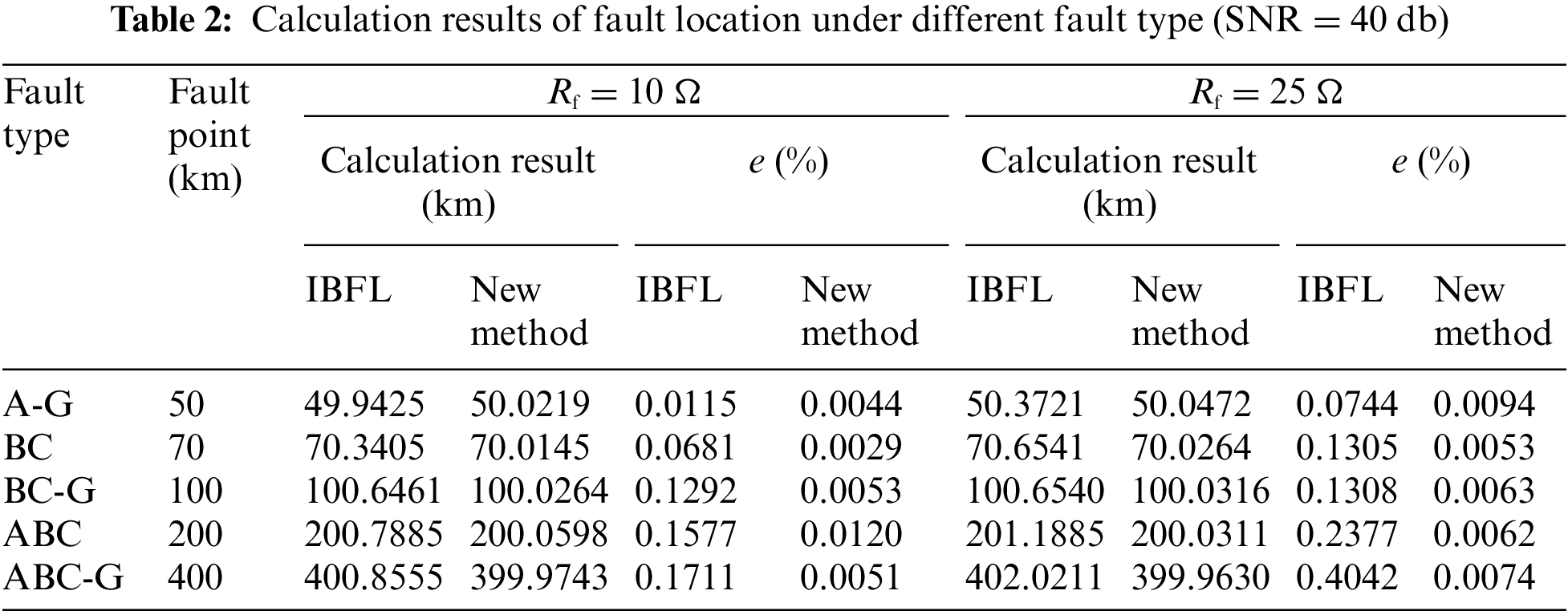
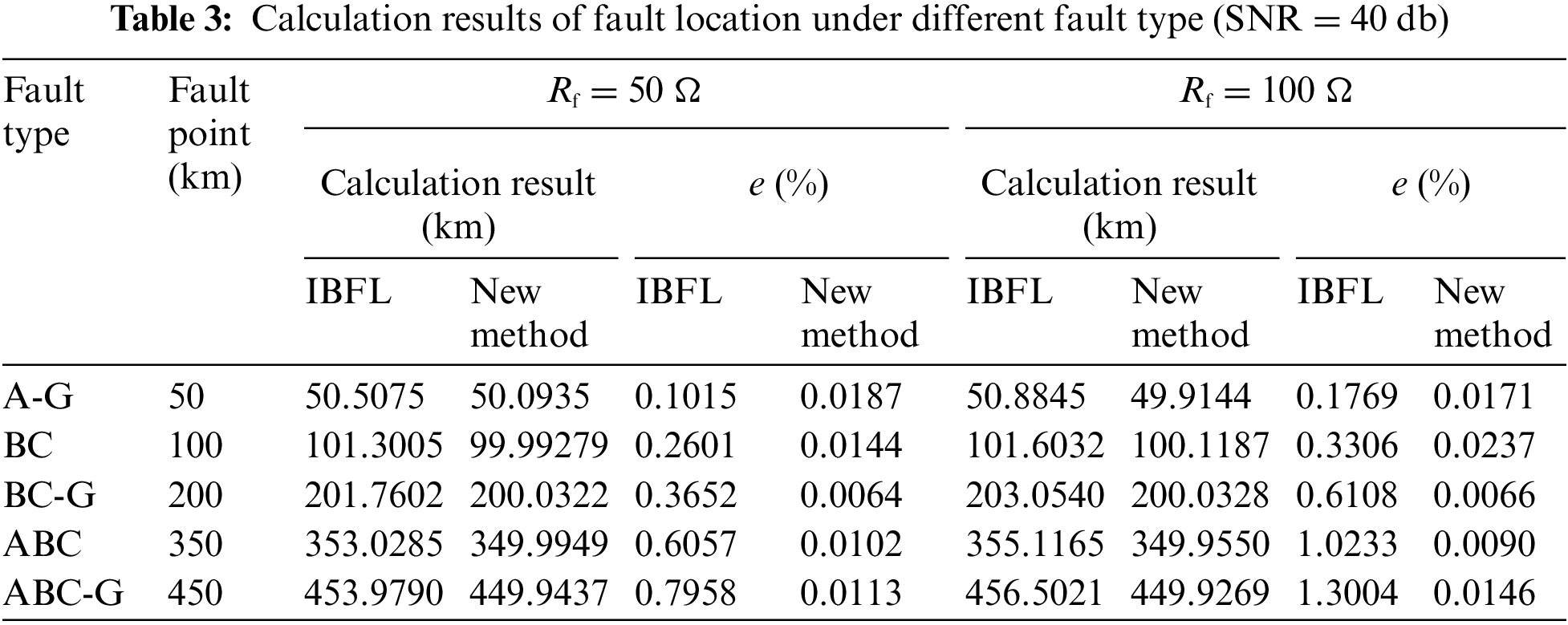
From the simulation results, the new method proposed in this paper has greatly improved the fault location accuracy of all fault types compared with the traditional IBFL method. Since the calculation of the fundamental frequency impedance in the traditional IBFL method requires zero-sequence current compensation, the calculation result of the fundamental frequency impedance is affected by the transition resistance, the operation mode and the opposite system impedance, and the centralized parameter model is used for the transmission line, which will inevitably lead to the fault location accuracy loss. The new method proposed in this paper can effectively overcome the influence of transition resistance, operation mode and system impedance, and the distributed parameter model is used for the transmission line, which can achieve high-precision fault location.

5.2 Correlation Analysis between el and ec

As the actual transmission line is greatly affected by the changes of external geographical and meteorological conditions for a long time, so its capacitance parameters will change, which will affect the accuracy of fault location results. Fig. 7 shows the correlation curve between the relative error of fault location (el) and capacitance parameters (ec), then el and ec are expressed as percentages.

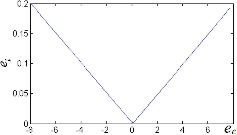
Figure 7: Correlation curve between el and ec

It can be seen from Fig. 7 that there is a typical linear correlation between el and ec. When the |ec|≤2%, the el≤0.05%, and the el is within the acceptable range, the results of fault location can still maintain high accuracy.

6  Conclusion

Based on the distributed parameter transmission line model, a new fault location algorithm for T-shaped transmission line based on phase angle jump checking is proposed in this paper. Firstly, the 3-terminal synchronous fundamental positive sequence voltage and current phasors are substituted into the fault branch distance function to realize the selection of fault branch when the fault occurs; Secondly, all roots (including real roots and virtual roots) are calculated by using the condition that the fundamental positive sequence voltage phasor at the fault point is equal. Finally, the verification calculation is performed by phase angle jump checking to determine that the only real root is the actual fault distance, Then the purpose of high-precision fault location is realized.

The algorithm has the characteristics of strong universality, high ranging accuracy and immunity to transition resistance. The simulation results verify the feasibility and effectiveness of the algorithm, and has a good application prospect.

CRediT Authorship Contribution Statement: Jia'an Xie: Data curation, Investigation, Resources, Software, Validation, Writing–original draft. Guobin Jin: Conceptualization, Methodology, Supervision. Yurong Wang: Review & editing, Project administration, Funding acquisition. Mucheng Wu: Simulation model building & review.

Funding Statement: This work is supported by National Nature Science Foundation of China (51507031).

Conflicts of Interest: The authors declare that they have no conflicts of interest to report regarding the present study.

References

 1.  Wang, Z. L., Liu, M. G. (2014). Traveling wave fault location for teed transmission line based on solutions of linear equations. Power System Technology, 38(4), 1046–1050. [Google Scholar]

 2.  Chen, X., Zhu, Y. L., Zhao, X. S. (2015). Traveling wave fault location for T-shaped transmission line considering change of line length. Power System Technology, 39(5), 1438–1443. [Google Scholar]

 3.  Ding, J. L., Wang, X., Zheng, Y. H. (2018). Distributed traveling-wave-based fault-location algorithm embedded in multi-terminal transmission lines. IEEE Transactions on Power Delivery, 33(6), 3045–3054. DOI 10.1109/TPWRD.2018.2866634. [Google Scholar] [CrossRef]

 4.  Chen, X., Zhu, Y. L., Gao, Y. F. (2016). A new fault location algorithm for high-voltage three-terminal transmission lines based on fault branch fast identification. Automation of Electric Power Systems, 40(4), 105–110. [Google Scholar]

 5.  Jin, X. N., Wang, F. P., Wang, Z. J. (2013). Research on fault location based on dynamic synchronous phasor measurement by PMU. Power System Technology, 37(7), 2932–2937. [Google Scholar]

 6.  Zhang, S. Q., Li, Y. L., Chen, X. L. (2018). A new fault location algorithm based on positive sequence current difference for double-circuit three-terminal transmission lines. Proceedings of the CSEE, 38(5), 1488–1495. [Google Scholar]

 7.  Shi, S. H., He, B. T., Zhang, W. J. (2008). Fault location for HV three-terminal transmission lines. Proceedings of the CSEE, 28(25), 105–110. [Google Scholar]

 8.  Lin, F. H., Wang, Z. P. (2011). Fault locating method based on two-terminal common positive sequence fundamental frequency component for parallel transmission line. Proceedings of the CSEE, 31(4), 93–98. [Google Scholar]

 9.  Tan, D., Yang, H. G., Qu, G. L. (2012). Fault location for distribution network based on fault distance distribution function. Power System Technology, 36(10), 119–124. [Google Scholar]

10. Hong, Y. S., Wen, J. Z., Yu, B. D. (2013). A new PMU-based fault location algorithm for three-terminal. Advanced Materials Research, 634–638, 3925–3929. [Google Scholar]

11. Lin, F. H., Wang, Z. P., Zeng, H. M. (2011). A novel fault location algorithm based on phase characteristics of fault location function for three-terminal transmission lines. Proceedings of the CSEE, 31(13), 107–113. [Google Scholar]

12. Lin, Y. H., Liu, C. W., Yu, C. S. (2002). A new fault locator for three-terminal transmission lines using two-terminal synchronized voltage and current phasors. IEEE Transactions on Power Delivery, 17(2), 452–459. DOI 10.1109/61.997917. [Google Scholar] [CrossRef]

13. Liu, R. L., Tai, N. L., Fan, C. J. (2018). Research on accurate fault location for multi-terminal transmission lines based on positive sequence components. Power System Technology, 42(9), 3033–3040. [Google Scholar]

14. Wei, G., Tang, B., Xiao, H. J. (2001). New location method of unbalanced faults on transmission lines. Automation of Electric Power Systems, 25(17), 29–31. [Google Scholar]

15. Zhou, D. M. (1998). A practical approach to accurate fault location on 3-terminal power system. Electric Power Automation Equipment, 18(1), 17–20. [Google Scholar]

16. Kang, X. N., Suonan, J. L. (2005). Frequency domain fault location method based on the transmission line parameter identification using two terminal data. Automation of Electric Power Systems, 29(10), 16–20. [Google Scholar]

17. Hong, Y., Tan, Y. H., Zhang, H. X., Song, J. L. (2016). Fault location algorithm of transmission line based on two-terminal electrical power quantities. Proceedings of the CSU-EPSA, 28(11), 20–24. [Google Scholar]

18. Wang, F. H., Mu, K., Zhang, J. (2018). Asynchronous two-terminal fault location method of transmission line based on parameter modification. Electric Power Automation Equipment, 38(8), 95–101. [Google Scholar]

19. Chen, X., Zhu, Y. L., Guo, X. H. (2016). Dual-terminal asynchronous fault location algorithm for two parallel overhead lines on same pole. Electric Power Automation Equipment, 36(5), 87–90. [Google Scholar]

20. Chen, X., Zhang, L. H., Zhang, X. R. (2020). Asynchronous fault location algorithm for T-shaped transmission line considering characteristics of location result. Automation of Electric Power Systems, 42(21), 132–138. [Google Scholar]

21. Ren, H. X., Liang, R., Ding, R., Xin, J. (2015). Fault location research adopted two-terminal asynchronous data and based on accurate line-searching and phase-comparing. Power System Technology, 39(10), 2972–2978. [Google Scholar]

22. Jia, K., Dong, X. Y., Li, L. (2020). Fault location for distribution network based on transient sparse voltage amplitude measurement. Power System Technology, 44(3), 835–844. [Google Scholar]

23. Li, Z. X., Wang, X., Tian, B. (2018). A fast fault location method based on distribution voltage regularities along transmission line. Transactions of China Electrotechnical Society, 33(1), 112–120. [Google Scholar]

24. Chen, X., Zhu, Y. L., Guo, X. H. (2015). A two-terminal fault location algorithm using asynchronous data based on phase characteristics for high voltage transmission line. Automation of Electric power systems, 39(22), 152–156. [Google Scholar]

This work is licensed under a Creative Commons Attribution 4.0 International License, which permits unrestricted use, distribution, and reproduction in any medium, provided the original work is properly cited.