Energy Engineering

---

DOI: 10.32604/ee.2022.020490

ARTICLE

Anomaly Detection and Pattern Differentiation in Monitoring Data from Power Transformers

Jun Zhao1, Shuguo Gao1, Yunpeng Liu2,3, Quan Wang2,*, Ziqiang Xu2, Yuan Tian1 and Lu Sun1

1State Grid Hebei Electric Power Research Institute, Shijiazhuang, 050021, China
2Hebei Provincial Key Laboratory of Power Transmission Equipment Security Defense, North China Electric Power University, Baoding, 071003, China
3State Key Laboratory of Alternate Electrical Power System with Renewable Energy Sources, North China Electric Power University, Beijing, 102206, China
*Corresponding Author: Quan Wang. Email: wangquan@ncepu.edu.cn
Received: 26 November 2021; Accepted: 15 February 2022

1  Introduction

With the extensive application of advanced sensor monitoring technology in the operation and maintenance of power transformers, the scale of transformer monitoring data shows an exponential trend in its growth, providing an important data foundation for the comprehensive state assessment and prediction of equipment; however, affected by various emergencies, an equipment on-line monitoring system will inevitably generate some abnormal data. According to the operating characteristics of the transformer, the abnormalities in the monitoring data are mainly divided into invalid abnormal data and valid abnormal data.

Invalid abnormal data include missing values and noise. Missing values refer to data interruptions caused by short-term failure of the sensing device, abnormal communication ports, and recording errors; Noise refers to data that deviate from the expected value due to factors such as unstable operation of monitoring equipment and external environmental interference. Data cleaning measures should be taken against invalid abnormal data to ensure the smooth progress of subsequent equipment condition assessment. Valid abnormal data refer to the horizontal migration changes in the trend of monitoring data caused by sudden failures and insulation degradation during operation of the equipment. Valid abnormal data contain key information about abnormal changes in the equipment state, reflecting the true performance of the equipment operating state, so it does not come within the ambit of the processing category of data cleaning.

Reliable identification of abnormal data and effective differentiation of abnormal patterns are important foundations for achieving on-line monitoring data cleaning and an accurate understanding of equipment operating status. In the anomaly data identification process, time series decomposition [1], time series transformation [2], statistics based and clustering based methods are mainly used. Reference [3] constructed a robust covariance estimator through the idea of iteration and Mahalanobis distance and uses this as a basis to calculate robust correlation parameters, thereby achieving effective detection of transformer oil chromatography outliers. Reference [4] proposed an abnormal detection method for power equipment status data. The basic principle is to use the iterative test method of model fitting residuals to extract abnormal information in the data, and to detect missing data and correct noise data. Reference [5] used a fuzzy C-means clustering algorithm to cluster power equipment data according to different time windows and set the anomaly score of each cluster to judge whether the data are abnormal or not.

To obtain an accurate understanding of changes in the status of a power transformer and avoid the key information pertaining to any abnormal state from being mistakenly cleaned, it is necessary to conduct an in-depth analysis around the problem of pattern differentiation, however, there are few related research results. Reference [6] used the DBSCAN clustering algorithm to identify abnormal data in the sequence. On this basis, a data cleaning process framework considering the correlation of the time series is constructed to achieve effective distinction between abnormal sensor data and abnormal equipment status. Reference [7] proposed a data cleaning method for power equipment based on a stacked denoising autoencoder, which can identify and repair outliers and missing information, and filter any interference data while distinguishing the abnormal operating state of the equipment.

The above-mentioned papers on abnormal data identification and pattern distinction mainly focus on the research of abnormal points, and do not take into account the differences in the overall characteristics of the sequence before and after the abnormal time under different abnormal patterns, which may easily lead to misjudgment of abnormal patterns. In the present work a complete anomaly detection technology framework was constructed for the problem wherein transformer monitoring data contain different types of anomaly data. First, the empirical wavelet transform (EWT), and autoregressive integrated moving average (ARIMA) model were used to model the monitoring data time series, and the residual sequence that can reflect the abnormal characteristics of the monitoring data is obtained by calculating the difference between the predicted value and the measured value. Then, use the isolated forest algorithm to perform abnormal recognition on the residual sequence, and use the recognition result as the segment boundary to segment the original sequence; Finally, the improved multi-dimensional SAX vector representation is used to represent the segment subsequence as the symbol vector. The similarity score of the two adjacent symbol vectors was calculated and combined with the decision threshold to realise anomaly pattern discrimination, and the assessment results were verified by using the sequence correlation. The effectiveness of this method is verified by testing data from an oil temperature and dissolved gas in oil of a 500-kV transformer. The research results can provide key technical support for the efficient cleaning of equipment monitoring data and accurate diagnosis of its operating status.

2  Abnormal Data Recognition Based on Time Series Modelling and Isolated Forest Algorithm

For the abnormal identification of transformer monitoring data, firstly, an EWT is used to adaptively decompose the original sequence into time series components with different frequencies; secondly, the time series components were modelled by ARIMA, and the predicted values of each component were reconstructed to obtain the predicted values of monitoring sequence; on this basis, the difference between predicted value and the measured value is calculated to obtain the residual sequence, and the abnormal data features will be clearly characterised in the residual sequence; finally, the isolated forest algorithm is used to extract abnormal information from the monitoring sequence.

2.1 EWT Theory

The EWT is a signal adaptive analysis method [8–10]. Compared with EMD and other decomposition methods, EWT algorithm has strong anti mode aliasing ability and short operation time. Taking a discrete signal in time domain as an example, the specific steps of EWT are as follows:

1)   Through the Fourier transform, the Fourier spectrum F(ω) of the input signal f(t) is obtained. ω is defined in the range [0, π].

2)   The Fourier spectrum of the signal is adaptively divided into N segments, and ωn (n = 1, 2, …, N) represents the boundary of the segment.

3)   N empirical wavelets were constructed on the basis of the Fourier spectrum segmentation. The empirical wavelet function and empirical scale function are given by Eqs. (1) and (2), and the values of β and γ by Eqs. (3) and (4).

ψ^n(ω)={1,(1+γ)ωn≤|ω|≤(1−γ)ωn+1cos⁡[π2β(12γωn+1(|ω|−(1−γ)ωn+1))],(1−γ)ωn+1≤|ω|≤(1+γ)ωn+1sin⁡[π2β(12γωn(|ω|−(1−γ)ωn))],(1−γ)ωn≤|ω|≤(1+γ)ωn0,others(1)

ϕ^n(ω)={1,|ω|≤(1−γ)ωncos⁡[π2β((12γωn|ω|−(1−γ)ωn))],(1−γ)ωn≤|ω|≤(1+γ)ωn0,others(2)

β(x)={0,x≤0x4(35−84x+70x2−20x3),∀x∈[0,1]1,x≥1(3)

γ<minn⁡(ωn+1−ωnωn+1+ωn)(4)

4)   The detailed coefficients and approximate coefficients were obtained through the following operations:

Wfe(n,t)=⟨f(t),ψn(t)⟩=F−1[f^(ω)ψ^n(ω)¯](5)

Wfe(0,t)=⟨f(t),ϕ1(t)⟩=F−1[f^(ω)ϕ^1(ω)¯](6)

5)   Reconstruct the original signal according to Eq. (7) and obtain the original signal decomposition results f0(t), fk(t).

f(t)=Wfε(0,t)∗ϕ1(t)+∑n=1NWfε(n,t)∗ψn(t)(7)

f0(t)=Wfe(0,t)∗ϕ1(t)(8)

fk(t)=Wfe(k,t)∗ψk(t)(k=1,2,…,N−1)(9)

Taking a 500-kV main transformer as an example, the top-layer oil temperature monitoring sequence with a length of 426 is processed by EWT to obtain four sets of modal components. The specific decomposition results are shown in Fig. 1.

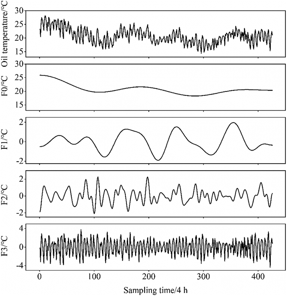
Figure 1: EWT decomposition results of oil temperature series

2.2 Autoregressive Integrated Moving Average Model

The ARIMA model is usually referred to as ARIMA (p, d, q) [11]. It is used to perform a d-order difference for a non-stationary time series to make it a stationary time series, then use an autoregressive moving average model (ARMA) to model this stationary series, and then obtain the original sequence after inversion.

Firstly, the stationarity test of input time series is needed to determine the value of difference order. In the present work, the construction test statistics were selected for hypothesis testing to determine the stationarity of the input time series. For non-stationary time series, it is necessary to repeat the difference process until the processed time series is stabilised. The difference processing process for a non-stationary time series {xt} is as follows:

∇dxt=(1−B)dxt(10)

where, B is the delay operator; ∇ = 1−B is the ordered difference operator; d represents the difference order.

The non-stationary time series {xt} is transformed into a stationary time series {yt} through difference processing. On this basis, the ARMA(p, q) model is established:

y^t=∑i=1pφiyt−i+εt−∑j=1qθjεt−j(11)

where, y^t represents the predicted value at time t; p and q represent the order of the autoregressive term and moving average term in the model; φi represents the coefficient of the ith autoregressive term; θj is the coefficient of the jth moving average; {εt} represents an independent normally distributed white noise sequence.

The construction of the ARMA model includes model ordering and parameter estimation. In the present work, the maximum likelihood method is used to estimate the parameters of the model. Based on the Akaike information criterion (AIC) [12], by limiting the value range of p and q, the order combination that minimises the AIC value is selected as the result of model order determination.

The monitoring sequence of transformer is decomposed by EWT theory, and the ARIMA prediction model is constructed through use of the aforementioned steps for the modal components obtained by the decomposition. To ensure the prediction accuracy of the ARIMA model, the component values were predicted in one step. By sliding the fitting window and the prediction window to the right with time, the complete prediction sequence about the modal components can be obtained; and then the predicted results of each component were reconstructed to obtain a complete prediction sequence of the monitoring data.

2.3 Isolation Forest Theory

EWT and ARIMA models were used to obtain the predicted values of monitoring indicators, which are subtracted from the actual measured values to obtain the residual items at the corresponding time, as given by Eq. (12). The residual sequence eliminates the periodic and trending effects of the original sequence in the process of change, making the residual term fluctuate around zero. Therefore, abnormal data caused by various emergencies will be more clearly expressed in the residual sequence in the form of outliers.

rest=x^t−xt(12)

The isolation forest (iForest) algorithm is an unsupervised anomaly detection method for continuous data [13]. Unlike distance-based and density-based anomaly detection methods, the isolated forest algorithm does not rely on any distance or density measurement, which significantly reduces the operating cost and has the advantages of high accuracy and high calculation efficiency [14]. Therefore, in this work the isolated forest algorithm was chosen to perform anomaly recognition on the residual sequence.

The isolated forest is composed of multiple isolated trees (iTree). The structure of iTree is as follows:

1)   Randomly select n training datapoints as a sub-sample set and put it into the root node of the tree.

2)   Specify an attribute dimension randomly, and randomly generate a cutting point s between the maximum and minimum values of the attribute dimension.

3)   Use this cutting point to generate a hyperplane to divide the current nodal data space to obtain two sub-sample spaces, put data less than s into the left branch of the current node, and put data greater than or equal to s into the right branch of the current node.

4)   Repeat Steps 2 and 3 to construct new subspace nodes until the data itself cannot continue to be split or the depth limit of the isolated tree is reached.

An isolated forest with multiple isolated trees was thus established so that abnormal data can be detected based on the path length h(x) of the sample in each isolated tree. Due to their particularity, abnormal data can usually be separated early to reach external nodes with a small path length; normal data can only be separated after multiple binary tree classifications, and the path length is large. Therefore, the degree of abnormality of data can be judged by the anomaly score s(x, n), as given by:

c(n)=2H(n−1)−2(n−1)n(13)

S(x,n)=2−E[h(x)]c(n)(14)

where, H(i) represents the harmonic number, its value can be estimated as ln(i) + ξ, where ξ is Euler’s constant; c(n) represents the average path length after a given number of samples, and is used to normalise the path length of the samples; E(h(x)) represents the average path length of sample point x on all isolated trees.

When s(x, n) approaches 1, it indicates that the sample point is more likely to represent an abnormal datum; when s(x, n) approaches 0, it indicates that the sample point is more likely to normal.

3  Distinguishing Abnormal Patterns in Monitoring Data

After effective extraction of abnormal data information, the accurate determination of any abnormal patterns can be realised. Invalid anomaly patterns mainly include noise and missing values. At the moment when an anomaly occurs, the observed value will deviate significantly from the expected value, and the time series before and after this time will retain relatively consistent characteristics; the effective abnormal mode mainly refers to the horizontal migration and trend change of monitoring data caused by abnormal changes in equipment status, and the time series characteristics before and after the abnormality differ significantly, therefore, on the basis of dividing the time sequence by using the abnormal point as segment point, an improved multi-dimensional SAX vector representation method is introduced to perform multi-dimensional symbolic vector representation of the segmented sub-sequence. Then, by calculating the similarity score of two adjacent symbol vectors and combining these with the decision threshold to distinguish different abnormal patterns, and further use sequence correlation analysis to verify the results of pattern determination.

3.1 Abnormal Pattern Judgment Based on Improved Multi-Dimensional SAX Vector Representation Method

3.1.1 Improved Multi-Dimensional SAX Vector Representation Method

Symbolic aggregation approximation (SAX) is commonly used for symbolic representation of time series [15]. The traditional SAX method takes the mean value of each time series as the representative feature of the segmented series from the segmented time series. Considering the greater limitations of the mean representation method, users have improved the traditional SAX method by perfecting the time series feature representation to good effect [16,17]. The improved multi-dimensional SAX vector representation method adopted here considers the statistical characteristics, morphological characteristics, and entropy characteristics of the time series [18], selects the mean value, slope, and sample entropy to form the eigenvalue vector to represent the series characteristics completely. The specific process includes:

1)   Z-score standardisation of the time series

Z-score standardisation can transform data of different orders of magnitude into the value of unified measurement to ensure comparability of data.

2)   Segment the time series equidistantly and express their eigenvalues

The normalised time series are divided into equidistant segments, and mean value, slope, and sample entropy are selected as the eigenvalues of the time series to construct the eigenvalue vector that can fully characterise the time series.

3)   Symbolic vector representation of time series

According to the numerical distribution of time series eigenvalues, the numerical space between each type of eigenvalue is divided with equal probability, and different characters are used to represent the divided numerical subspace regions, such as the letter set {A, B, C, D, E, …}. Let the scale parameter of the set be α, and the larger the value of α, the higher the accuracy of division of the numerical space. Normally, the range of α is [3,19]. The time series follows a Gaussian distribution after z-score normalization. According to the value of α, query the corresponding segment points in the Gaussian distribution table. For example, when the value of α is 3, by querying the Gaussian distribution table, select −0.43 and 0.43 as the segment points, and divide the numerical space into three equal-probability parts. Here, the character sequences representing the mean, slope, and sample entropy characteristics are respectively denoted by A^, S^, and E^.

Taking 60 sets of top oil temperature monitoring data of a 500-kV main transformer as an example, the process of multi-dimensional symbolic vector representation is realised. First, the monitoring sequence is normalised by Z-score (Fig. 2).

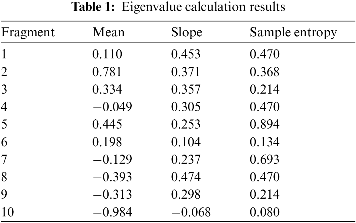
Then, the normalised monitoring sequence is divided into 10 segments at equal intervals, and the mean, slope, and sample entropy of each segmented sequence are calculated (Table 1).

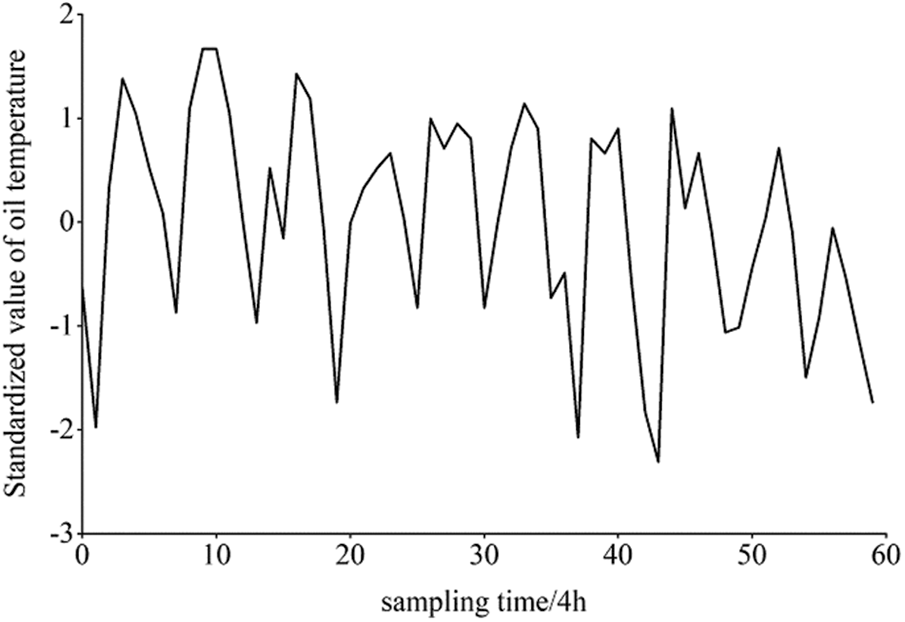
Figure 2: Z-score standardised top oil temperature sequence

Furthermore, the numerical space of various eigenvalues is divided into equal probabilities with α set to 20, and all subspaces represented by letters “A” to “T” from bottom to top.

Finally, the symbolic representation of the oil temperature sequence eigenvalues is obtained (Fig. 3), where the character sequences of mean, slope, and sample entropy are respectively expressed as “KPMJNLJGHD”, “NMMMLLLNMJ”, and “NMLNQKPNLK”.

In summary, a three-dimensional real vector space was constructed by improving the SAX vector representation method. The three dimensions in the space represent the three eigenvalues of mean, slope, and sample entropy, respectively. Therefore, the characteristics of each sub-segment of the time series can be represented by a symbol vector in three-dimensional space, for example, q→i=(A^i,S^i,E^i) is used to characterise the ith sub-segment of the time series.

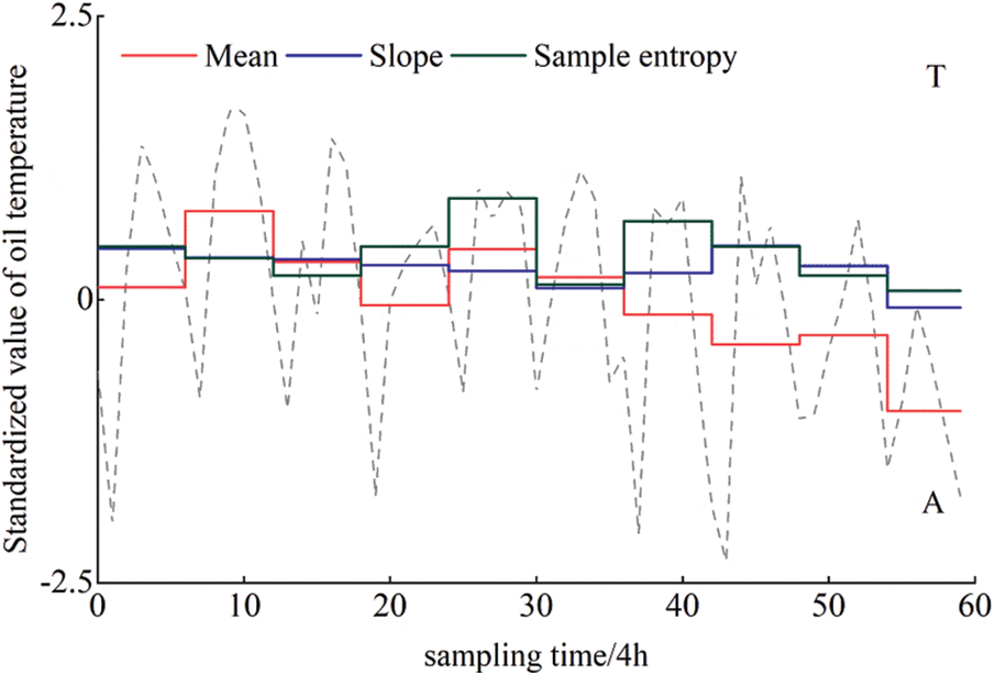
Figure 3: Symbolic representation of top oil temperature sequence eigenvalues

3.1.2 Similarity Calculation and Abnormal Pattern Determination

Through the aforementioned steps, the multi-dimensional symbolic vector representation of each segmented subsequence is realised. When the abnormal point belongs to a valid abnormal mode, the characteristics of the sub-sequences on the left and right sides of the abnormal point will differ greatly; while when the abnormal point belongs to the invalid abnormal mode, the sub-sequences on the left and right sides of the abnormal point will maintain more consistent characteristics. Therefore, by calculating the similarity values of the symbol vectors of the sub-sequences on both sides of the abnormal point to determine the anomaly pattern, the specific process is as follows:

1)   For a segment boundary, the lengths of the multi-dimensional symbolised vectors of the sub-sequences on both sides are compared. Then take the multi-dimensional symbolic vector sequence (L¯) of the longer sequence (L) as the sequence to be matched, and take the multi-dimensional symbolic vector sequence (Q¯) of the shorter sequence (Q) as the target template sequence.

2)   Move the target template sequence (Q¯) on the sequence to be matched (L¯), as shown in Fig. 4 and calculate the similarity score of the two at each position during the movement, as given by Eqs. (15) and (16). The minimum value in the similarity score set is selected as the abnormal mode judgment score of the segment point.

dist(L→i,Q→i)=(dist(A^iL,A^iQ))2+(dist(S^iL,S^iQ))2+(dist(E^iL,E^iQ))2(15)

MINDIST(L¯,Q¯)=1w∑i=1wdist(L→i,Q→i)(16)

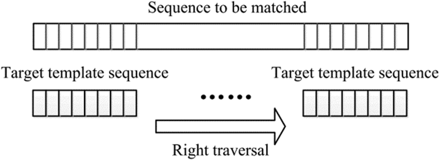
Figure 4: Moving of the target template

where, w represents the length of the target template sequence; dist() represents the measurement function of the character distance. According to the reference [16], the distance between any two characters can be obtained by looking up the table. Compared with the numerical calculation without symbolic representation, the conclusion is consistent, but the symbolic representation can improve the calculation efficiency.

3)   Set the threshold T for abnormal mode determination. If the score here is greater than T, the abnormal point is determined to be a valid abnormal mode; if the score is less than T, the abnormal point is determined to be an invalid abnormal mode.

4)   Repeat the above steps until the abnormal patterns of all abnormal points in the monitoring sequence are determined.

Based on the example given here, through several similarity retrieval experiments in advance, it is found that the similarity score of two groups of sequences with relatively consistent pattern is stable and below 0.5, therefore, the pattern decision threshold was set to 0.5; however, considering the limitation of threshold setting, sequence correlation analysis was introduced to verify further the results of pattern differentiation on the basis of using thresholding to distinguish abnormal patterns.

3.2 Sequence Correlation Analysis Based on the Grey Correlation Algorithm

The commonly used methods for time series correlation analysis include the Apriori algorithm [6], grey correlation analysis algorithm [19,20], and so on. Considering that the Apriori algorithm needs to traverse the database multiple times during operation, it suffers from low efficiency and slow solution. Here, the grey correlation algorithm was chosen to analyse the degree of correlation between each monitoring sequence.

The grey correlation analysis algorithm judges the strength of the correlation between parameters according to the similarity of the geometric shapes of the parameters. Through quantitative analysis of the development trend of the dynamic process, the algorithm completes the comparison of the geometric relationships between the time series and calculates the degree of correlation between the parameters.

Here, the reference sequence is denoted by {xt0|t=1,2,3,…,N} and the comparative sequence is denoted by {xti|t=1,2,3,…,N}, (i = 1, 2, 3,…, m). Considering the different physical meanings of the monitoring sequences, these sequences must be dimensionless:

yti=xti−xminixmaxi−xmini(17)

On this basis, the correlation coefficients of the corresponding elements of the comparison series and the reference series are calculated:

ζi(t)=mini⁡mint⁡|yt0−yti|+ρmaxi⁡maxt⁡|yt0−yti||yt0−yti|+ρmaxi⁡maxt⁡|yt0−yti|(18)

where, ρ is the distinguishing coefficient, usually taken as 0.5.

According to the grey correlation coefficients at each time point, the grey correlation degree between the reference sequence and the ith comparison sequence can be obtained:

ri=1N∑t=1Nζi(t)(19)

The greater the value of ri, the stronger the correlation between the comparison sequence and the reference sequence. We then set the correlation threshold rm to 0.75 and take the comparison sequence therewith as the correlation sequence.

3.3 Technical Framework for Monitoring Data Anomaly Detection

An abnormal detection technology framework for transformer monitoring data was constructed: it includes abnormal recognition and pattern determination function modules, as shown in Fig. 5, and the specific detection process is summarised below:

1)   The grey correlation analysis algorithm is used to measure the correlation between the sequence to be detected and other monitoring sequences. If there is a correlation sequence, the verification link is retained in the process of determining its abnormal pattern; if there is no correlation sequence, the verification link is removed.

2)   EWT theory is used to decompose the monitoring sequence, and the ARIMA prediction models are established for the modal components obtained from the decomposition. On this basis, the predicted results for each component are reconstructed to obtain the prediction sequence pertaining to the monitoring-data sequence.

3)   The residual sequence is obtained by calculating the difference between the predicted value and the actual value and the iForest algorithm is used to identify abnormal points in the residual sequence. These abnormal points are then used to segment the original monitoring sequence.

4)   The improved multi-dimensional SAX vector representation method is used to multi-dimensionally symbolise the segmented sequence and calculate the similarity scores of the symbol vectors on both sides of each abnormal point, so that different abnormal patterns are distinguished by combining the decision threshold.

5)   From the perspective of ensuring the safe and stable operation of the equipment, when an abnormal point of the monitoring sequence is determined to be an invalid abnormal mode, it is necessary to verify the determination by combining with the correlation sequence. If there is no abnormal point in the correlation sequence of the monitoring sequence at the same or adjacent time, the abnormal point can be determined as being an invalid abnormal pattern; if there is abnormal point in the correlation sequence at the same, or an adjacent time, the abnormal point is classified as a valid abnormal pattern, and the abnormality may have been due to an abnormal change in the operating state of the power transformer, or the related monitoring quantity is simultaneously subject to interference from external factors during the measurement or transmission process, which requires further intervention and judgment of staff.

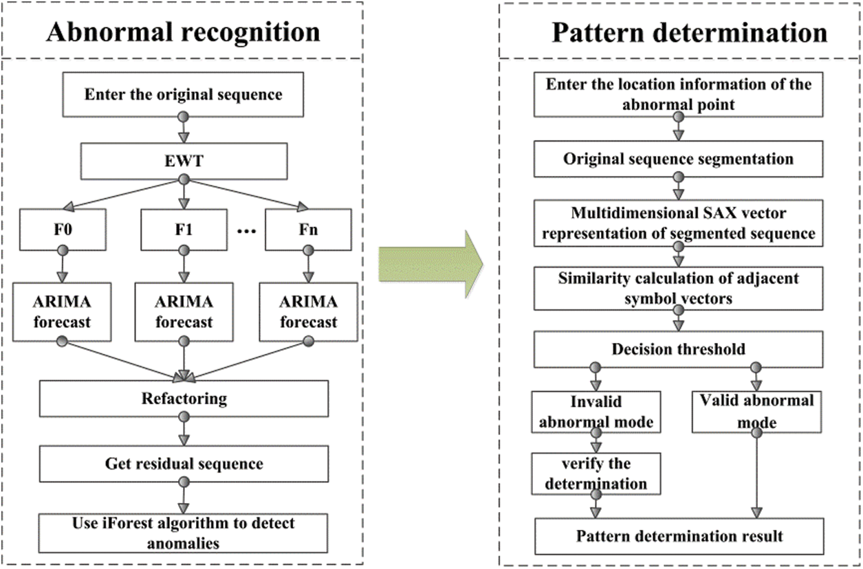
Figure 5: Flowchart for anomaly detection

4  Case Analysis

To verify the effectiveness of the proposed anomaly detection method, the on-line monitoring data from a 500-kV transformer in a substation collected 8 from November 2017 to 17 January 2018 are used as an example for analysis. The on-line monitoring data include seven parameters such as H2 concentration, top layer oil temperature, and load. The sampling interval of each monitoring parameter is 4 h, so each time series contains 426 data points.

4.1 Case 1

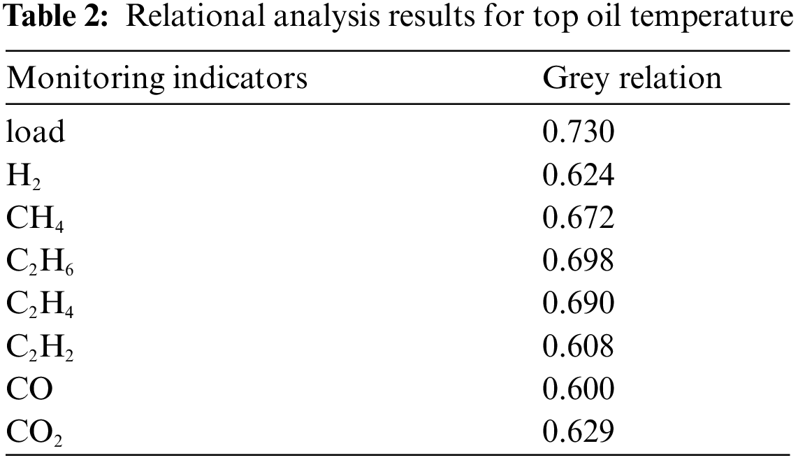
Taking the top layer oil temperature monitoring sequence as an example for analysis, according to the detection process described above, the grey correlation algorithm is used to calculate the correlation between it and other monitoring sequences. According to the calculated results (Table 2), the grey correlation between the oil temperature sequence and other monitoring sequences is less than the threshold rm. Therefore, in the pattern determination process, the verification link is removed, that is, only this single sequence is used for anomaly detection analysis.

The oil temperature sequence to be detected is shown in Fig. 6a, and there are no abnormal points in this sequence. To test the practicability of the proposed anomaly detection method, a sequence containing anomalies is formed by adding missing values and noise points to the original monitoring data. We set the monitoring value at the 230th sampling point to 0 as a missing value and added noise at the 172nd and 412th sampling points. The processed sequence is shown in Fig. 6b.

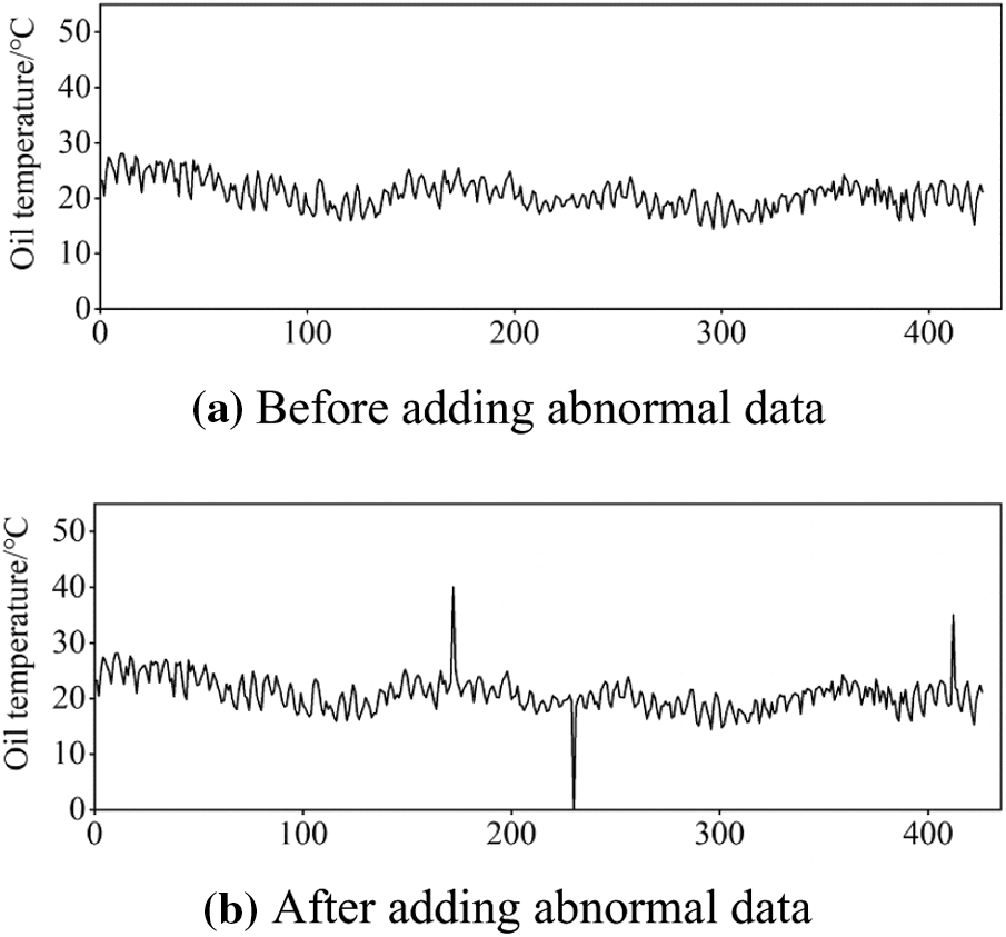
Figure 6: Monitoring data of top oil temperature

The oil temperature monitoring sequence after adding the abnormal point is modelled by EWT and ARIMA time series to obtain the residual sequence that can reflect the abnormal characteristics of the monitoring data (Fig. 7). Then, the iForest algorithm is used to identify the abnormal information from the residual sequence. The extracted abnormal points are located at the 172nd, 230th, and 412th sampling points of the monitoring sequence, which are consistent with the position of the abnormal points set here.

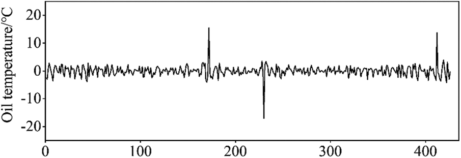
Figure 7: Residual error sequence of top oil temperature

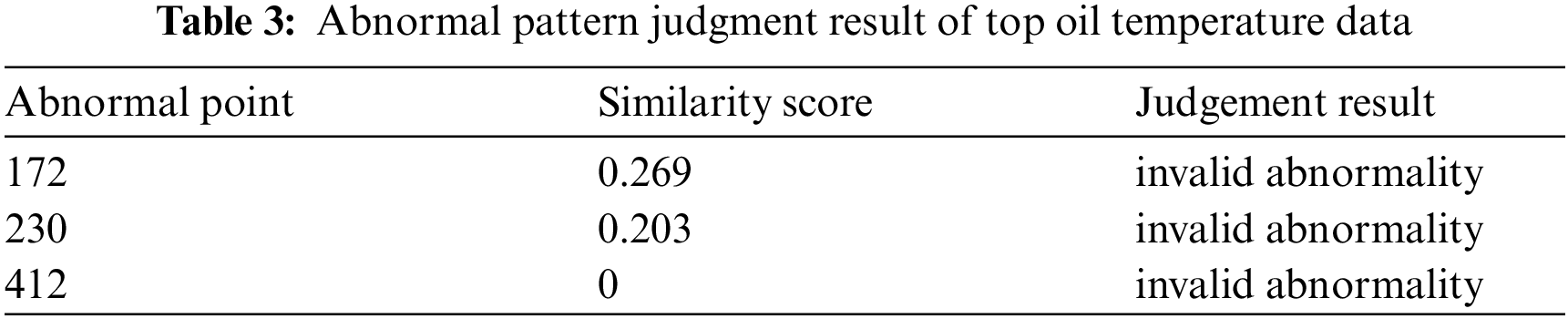
The sequence is segmented based on the aforementioned abnormal point position information, and each segment is expressed as a symbol vector using the improved multi-dimensional SAX vector representation method. Then, the similarity score of symbol vectors on both sides of each abnormal point is calculated. According to the calculated results in Table 3, combined with the decision threshold, the above three abnormal points are all invalid abnormalities, and the conclusion is consistent with the actual situation.

4.2 Case 2

Taking the data from the monitoring of C2H4 gas concentration as an example for analysis, the calculated grey correlations between C2H4 and other monitoring sequences are listed in Table 4: the correlation sequences of C2H4 concentration sequences include H2, CH4, C2H6, and C2H2 concentration sequences. Among them, the correlation between CH4 and C2H4 concentrations is the highest, and the on-line monitoring data of both are shown in Fig. 8. Therefore, in the process of distinguishing abnormal patterns, we should choose to retain the verification link, that is, combining the correlation sequence to determine the abnormal pattern.

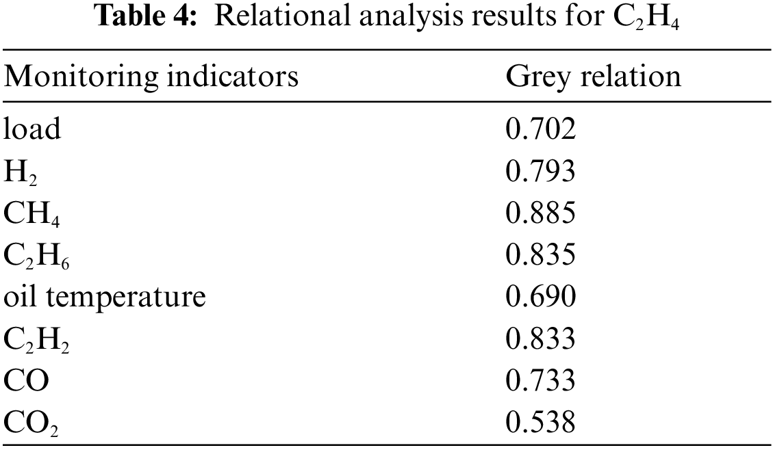
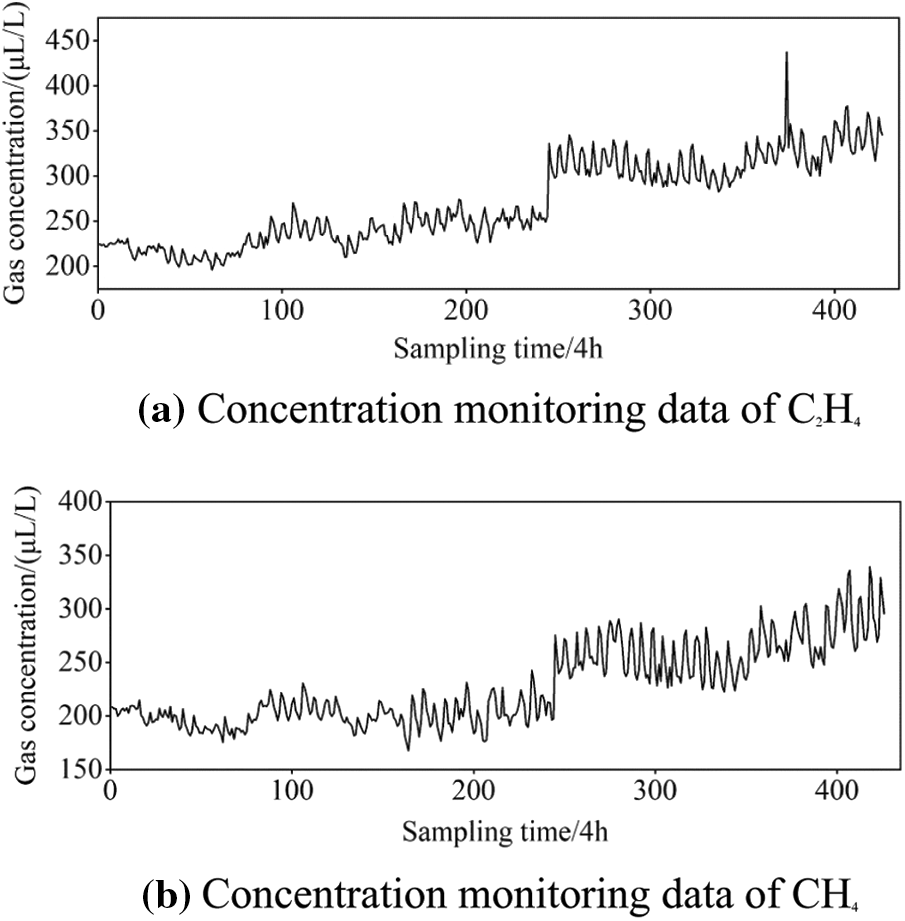
Figure 8: Concentration monitoring data of C2H4 and CH4

Using EWT theory and the ARIMA model to conduct time sequence modelling on the C2H4 concentration monitoring data, a residual sequence that can reflect the abnormal characteristics of the monitoring data is obtained (Fig. 9). The iForest algorithm is then used to perform anomaly recognition on the residual sequence, and the extracted anomaly points are located at the 245th and 380th sampling points of the monitoring sequence. On this basis, the above abnormal points are used as the segment points of the sequence and, on the basis of the improved multi-dimensional SAX vector representation method to complete the determination of the pattern of the abnormal points, the results are as listed in Table 5.

According to Table 5, the similarity score at the 380th sampling point of the C2H4 concentration sequence is 0.257, indicating that the time sequence characteristics before and after the abnormal moment are consistent, and, combined with the decision threshold, it is determined that it is an invalid abnormality pattern. In the process of result verification, the correlation sequence such as CH4 has no abnormal value at the same, or adjacent times, therefore, it can be concluded that there are noise data caused by factors such as external environmental interference or an unstable sensor device thereat.

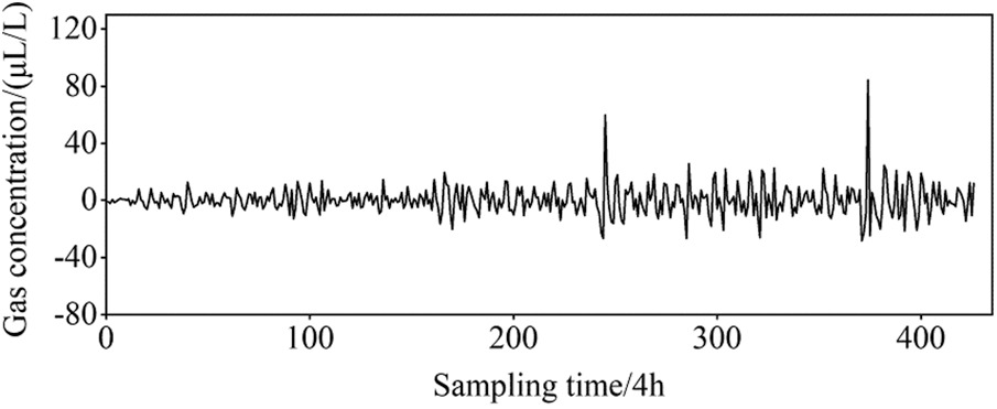
Figure 9: Residual error sequence of C2H4 concentration

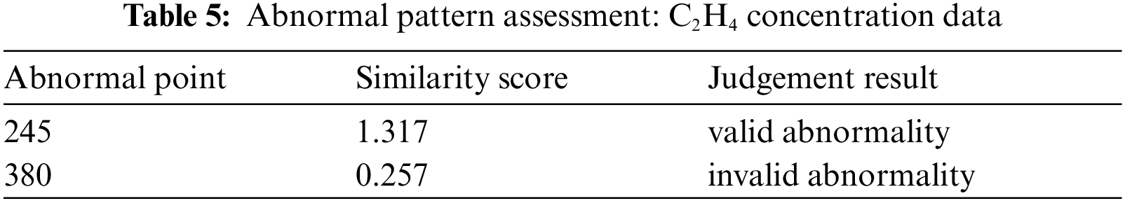
The similarity score at the 245th sampling point of the C2H4 concentration sequence is 1.317, indicating that the time series characteristics before and after the abnormal moment have changed to a significant extent, and, combined with the decision threshold, it is determined that it belongs to a valid abnormal mode. In addition, the associated CH4 concentration monitoring sequence also shows abnormal values at the same time, and the credibility of the above conclusion is further guaranteed. The actual situation at that time is that there are loose, hot parts inside the body of the power transformer, and the contact state is unstable, resulting in unstable staged high-temperature gas production. The results of the abnormal mode determination herein are consistent with the actual situation.

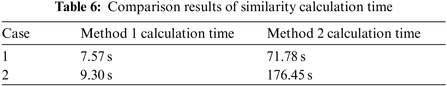
Finally, in the above two examples, we compare the similarity calculation time of each sub segment represented by symbol vector and the similarity calculation time of direct numerical calculation after segmentation, which proves that the improved multi-dimensional SAX vector representation method can significantly improve the computational efficiency. The former is denoted by Method 1 and the latter by Method 2. In Case 1 and Case 2, the calculation time of Method 1 is 10.55% and 5.27% of Method 2 respectively. The comparison of these results is shown in Table 6.

5  Conclusion

Aiming at the problem of abnormal data generated by abnormal changes in equipment status, external environmental interference and communication interruption in the power transformer on-line monitoring system, a method for abnormal detection and pattern differentiation of monitoring data was proposed. The following conclusions are drawn:

1)   Combined with EWT theory and ARIMA model, the online monitoring data were modelled to obtain the residual sequence that can reflect the abnormal characteristics of the monitoring data, and the iForest algorithm is then used to achieve the efficient extraction of abnormal information in the residual sequence.

2)   Based on the in-depth analysis of the difference between the invalid abnormal data and the valid abnormal data, the improved multi-dimensional SAX vector representation method is introduced to symbolise the time series. The similarity score of the symbol vector is then used to measure the difference in the characteristics of the segmented sequences on both sides of the abnormal point, combined with the decision threshold, the effective differentiation of abnormal patterns is realised.

3)   The grey correlation analysis algorithm was used to measure the correlation between monitoring sequences, and the results of an abnormal pattern assessment were further verified on the basis of the correlation between the time series, thus avoiding the limitations of decision threshold setting.

In summary, the proposed anomaly detection technology framework can provide key technical support for efficient cleaning of power transformer on-line monitoring data and accurate assessment of equipment operating status.

Funding Statement: This study was supported by State Grid Hebei Electric Power Co., Ltd. (kj2020-040).

Conflicts of Interest: The authors declare that they have no conflicts of interest to report regarding the present study.

References

 1.  Zhang, K., Shi, L., Hu, Y., Chen, P., Xu, Y. (2021). Variable spectral segmentation empirical wavelet transform for noisy signal processing. Digital Signal Processing, 117, 103151. DOI 10.1016/j.dsp.2021.103151. [Google Scholar] [CrossRef]

 2.  Zhang, K., Xu, Y., Liao, Z., Song, L., Chen, P. (2021). A novel fast entrogram and its applications in rolling bearing fault diagnosis. Mechanical Systems and Signal Processing, 154, 107582. DOI 10.1016/j.ymssp.2020.107582. [Google Scholar] [CrossRef]

 3.  Gao, S., Wang, X., Li, Q., Yang, R. (2014). Outliers detection and distribution characteristics of the transformer DGA data based on MCD robust statistics. High Voltage Engineering, 40(11), 3477–3482. DOI 10.13336/j.1003-6520.hve.2014.11.025. [Google Scholar] [CrossRef]

 4.  Yan, Y., Sheng, G., Chen, Y., Jiang, X., Guo, Z. et al. (2015). Cleaning method for big data of power transmission and transformation equipment state based on time sequence analysis. Automation of Electric Power Systems, 39(7), 138–144. DOI 10.7500/AEPS20140111003. [Google Scholar] [CrossRef]

 5.  Chen, J., Chen, Y., Yan, Y., Du, X., Sheng, G. et al. (2015). Anomaly detection of state information of power equipment based on spatiotemporal clustering. Southern Power System Technology, 9(11), 65–72. DOI 10.13648/j.cnki.issn1674-0629.2015.11.010. [Google Scholar] [CrossRef]

 6.  Lin, J., Yan, Y., Sheng, G., Jiang, X., Yang, Y. et al. (2017). Online monitoring data cleaning of transformer considering time series correlation. Power System Technology, 41(11), 3733–3740. DOI 10.13335/j.1000-3673.pst.2017.0141. [Google Scholar] [CrossRef]

 7.  Dai, J., Song, H., Sheng, G., Jiang, X. (2017). Cleaning method for status monitoring data of power equipment based on stacked denoising autoencoders. IEEE Access, 5, 22863–22870. DOI 10.1109/ACCESS.2017.2740968. [Google Scholar] [CrossRef]

 8.  Gilles, J. (2013). Empirical wavelet transform. IEEE Transactions on Signal Processing, 61(16), 3999–4010. DOI 10.1109/TSP.2013.2265222. [Google Scholar] [CrossRef]

 9.  Zhao, M., Xu, G. (2017). Feature extraction for vibration signals of power transformer based on empirical wavelet transform. Automation of Electric Power Systems, 41(20), 63–69 + 91. DOI 10.7500/AEPS20170327001. [Google Scholar] [CrossRef]

10. Liu, W., Chen, W. (2019). Recent advancements in empirical wavelet transform and its applications. IEEE Access, 7, 103770–103780. DOI 10.1109/ACCESS.2019.2930529. [Google Scholar] [CrossRef]

11. Box, G. E. P., Jenkins, G. M., Reinsel, G. C., Ljung, G. M. (2015). Time series analysis: Forecasting and control. John Wiley & Sons, USA. DOI 10.1111/j.1467-9892.2009.00643.x. [Google Scholar] [CrossRef]

12. Burnham, K. P., Anderson, D. R. (2004). Multimodel inference: Understanding AIC and BIC in model selection. Sociological Methods & Research, 33(2), 261–304. DOI 10.1177/0049124104268644. [Google Scholar] [CrossRef]

13. Liu, F. T., Ting, K. M., Zhou, Z. H. (2008). Isolation forest. Proceedings of the 2008 Eighth IEEE International Conference on Data Mining, pp. 413–422. Pisa, Italy. DOI 10.1109/ICDM.2008.17. [Google Scholar] [CrossRef]

14. Li, S., Zhang, K., Duan, P., Kang, X. (2019). Hyperspectral anomaly detection with kernel isolation forest. IEEE Transactions on Geoscience and Remote Sensing, 58(1), 319–329. DOI 10.1109/TGRS.2019.2936308. [Google Scholar] [CrossRef]

15. Lin, J., Keogh, E., Lonardi, S., Chiu, B. (2003). A symbolic representation of time series, with implications for streaming algorithms. Proceedings of the 8th ACM SIGMOD Workshop on Research Issues in Data Mining and Knowledge Discovery, pp. 2–11. San Diego, USA. [Google Scholar]

16. Sun, Y., Li, J., Liu, J., Sun, B., Chow, C. (2014). An improvement of symbolic aggregate approximation distance measure for time series. Neurocomputing, 138, 189–198. DOI 10.1016/j.neucom.2014.01.045. [Google Scholar] [CrossRef]

17. Li, H., Liang, Y. (2017). Similarity measure based on numerical symbolic and shape feature for time series. Control and Decision, 32(3), 451–458. DOI 10.13195/j.kzyjc.2016.0326. [Google Scholar] [CrossRef]

18. Wang, C. (2019). Research on prediction and anomaly detection algorithm of time series in cloud environment. Nanjing University, China. [Google Scholar]

19. Sima, L., Shu, N., Zuo, J., Wang, B., Peng, H. (2012). Concentration prediction of dissolved gases in transformer oil based on grey relational analysis and fuzzy support vector machines. Power System Protection and Control, 40(19), 41–46. [Google Scholar]

20. Liu, H., Wang, Y., Liang, X., Bai, D., Qin, J. (2018). Prediction method of the dissolved gas volume fraction in transformer oil based on multi factors. High Voltage Engineering, 44(4), 1114–1121. DOI 10.13336/j.1003-6520.hve.20180329010. [Google Scholar] [CrossRef]

This work is licensed under a Creative Commons Attribution 4.0 International License, which permits unrestricted use, distribution, and reproduction in any medium, provided the original work is properly cited.