Energy Engineering

---

DOI: 10.32604/ee.2022.020698

ARTICLE

Energy Efficient Thermal Comfort Control for Residential Building Based on Nonlinear EMPC

Xucheng Chang1,*, Bing Kong2, Yong Li1, Gaofeng Ren1, Chao Zhang1 and Zhenghe Wang1

1Zhengzhou University of Aeronautics, Zhengzhou, 450046, China
2Zhengzhou Technical College, Zhengzhou, 450010, China
*Corresponding Author: Xucheng Chang. Email: changxc@zua.edu.cn
Received: 17 November 2021; Accepted: 28 January 2022

1  Introduction

Energy-efficient and intelligent green buildings are becoming more and more important, with climate change and the reduction of fossil energy. Construction energy consumption includes the whole process energy cost in the three stages of building material manufacturing, building construction and building operation, while the energy cost of building operation is dominant, including the daily energy cost of residents, such as heating, lighting, cooking, air conditioning and household appliances. Energy cost in China's buildings totaled 899 million tons of standardized coal, approximatively 20.6 percent of the country's total energy cost in 2016, according to statistics. And the heating energy cost of northern cities and towns in China is approximately 193 million tons of standardized coal, approximately 21.47 percent of the total energy cost of buildings nationwide [1]. Therefore, it can effectively decrease the total energy cost of buildings by decreasing the energy cost in heating.

Central heating was widely used in northern China. Many policies, regulations and standards had been issued by national and local governments, as the energy problem was becoming more and more serious. For example, In December 2017, Henan Province issued the Energy Conservation Regulations of Henan Province [2], which pointed out that “new buildings and existing buildings should be equipped with heat metering conditions for household use, and have the possibility to realize heat meter metering and household control according to the heat meter”. Therefore, household control and heat metering were important measures to realize energy efficient in green buildings. Users could adjust the heating heat according to their own needs, so as to improve the thermal comfort and cut down the heating cost.

The Model Predictive Control (MPC) method has a good control effect. Therefore, there were many applications in indoor temperature, humidity and energy saving control using HVAC (Heating, Ventilation and Air Conditioning) or electric heating systems. Kajgaard et al. identified the room temperature model based on the measured room data by using the system identification method, and designed the rolling time controller (RHC) to control the room temperature to decrease the energy cost of the power supply, so as to achieve energy saving [3]. Mario et al. designed the optimal solution problem for the temperature control of household boiler heating system and obtained the optimal temperature of the heating medium and optimal mass flow based on the idea of MPC. And the purpose of minimizing the energy cost in a certain range was achieved [4]. Jozef et al. solved the temperature control problem of office buildings with characteristics of multi-variable systems, simplified the multi-variable system into multiple univariate systems, and designed a decoupled MPC controller, which eliminated the influence of frequent disturbances and improved the energy saving effect [5]. Takatoshi et al. used k-means clustering and robust outlier prediction method to predict solar radiation, and used MPC to control the temperature change of HVAC room, so as to obtain comfortable temperature and reduce electricity cost at the same time [6]. Yang et al. estimated the uncertain parameters in the building model by using the actual building operation data measured online, introduced the model adaptive function, and designed an adaptive robust controller. Compared with the constant temperature controller, the energy consumption was reduced by about 20% [7]. When controlling the thermal comfort of a room, Barata et al. designed a distributed MPC algorithm by solving multiple subsystems under their own state prediction and coupling constraints, which realized the saving of power cost [8]. Maciej et al. used the online secondary optimization calculation of MPC to realize the indoor temperature and reduce energy consumption control of the electric heating floor heating system [9].

Energy efficient was achieved, but the main position of human comfort in indoor thermal environment was ignored, in the control system with temperature control as the goal. Indoor thermal comfort could be adjusted by temperature regulation, but there was a certain lag in this control process, because this method indirectly affected the comfort of the human body [8–10]. Therefore, the comfort and energy efficient of the heating system under the traditional temperature control strategy need to be further developed and studied. The main work of this investigation is to propose an energy-saving control strategy that meets the thermal comfort conditions, and use computer simulation to verify the effect.

The chapter structure of this paper is as follows. In Section 2, the residential thermal room used in the simulation of this study is briefly described, and then the nonlinear thermal comfort model of the thermal room is described in detail. In Section 3, the structure of the control system is introduced, the approximate nonlinear prediction model and algorithm steps are given, and the economic cost function and optimization problem are designed. Section 4 summarizes and analyzes the simulation results of this study. Section 5 summarizes the research results.

2  Thermal Comfort Model

The control architecture and strategy were proposed based on the EMPC, with the view of maintaining appropriate thermal comfort, meanwhile, decreasing the energy cost of the heating room. The proposed control strategy was validated in the simulation, based on real data from given room and environment. Therefore, indoor dynamic models that can accurately describe the main environmental parameters needed to be established first. To be more exact, in this work, a thermal comfort model of heating room based on the energy conservation law was established.

2.1 Description of Residential Room for Simulation

A bedroom in the residential building, with a volume of 5 × 4 × 2.7 square meters and a south-facing window with double glazing and an area of 19.71 square meters, was selected as the research object for modeling and simulation control in this study. The room was heated in the same way as other surrounding rooms and there were no electronics that continuously heat the room. The radiator was used as a heating device in the room, and the hot water flow of the radiator was regulated by an electric valve located at the radiator entrance, and then the ambient temperature in the heating room and the thermal comfort expected by residential users was regulated. The windows of heating room were opened in a shorter time during the winter heating period.

2.2 Temperature Dynamic Model of Heat Conduction Process

In general, the heat conduction process of enclosed heating room was a complex system, and the environmental factors affecting the system mainly included two aspects, one was the indoor environment, and the other was the outdoor environment. Indoor environmental factors mainly included indoor heat dissipation equipment, windows and walls. Outdoor environmental factors mainly included external climate and micro-climate in surrounding rooms. The mathematical mechanism equation of different environmental factors could be described according to First Principle of Thermodynamics, and the quantity of heat in the equation included heat by heat convection, heat conduction and heat radiation [11]. Therefore, the dynamic temperature equation of indoor heat conduction process was described by Eq. (1),

maCaT˙ain=Qradiator+Qwindow+Qwall+QiGain+Qnvnt+Qinf(1)

According to Eq. (1), the heat involved in the calculation of indoor environmental temperature variables included:

(1)   the heat dissipation of the radiator Qradiator;

(2)   the heat conduction through the window Qwindow, including heat exchange with the outside environment and heat conduction of solar radiation through the glass;

(3)   the heat conduction through the wall Qwall, including heat conduction with the outside and adjacent room;

(4)   the internal environmental thermal gain generated by indoor personnel and electronic equipment QiGain;

(5)   the heat changes generated by natural ventilation Qnvnt;

(6)   the heat generated by thermal penetration through the gap of the door Qinf.

The representation of the heat balance inside a room was shown in Fig. 1.

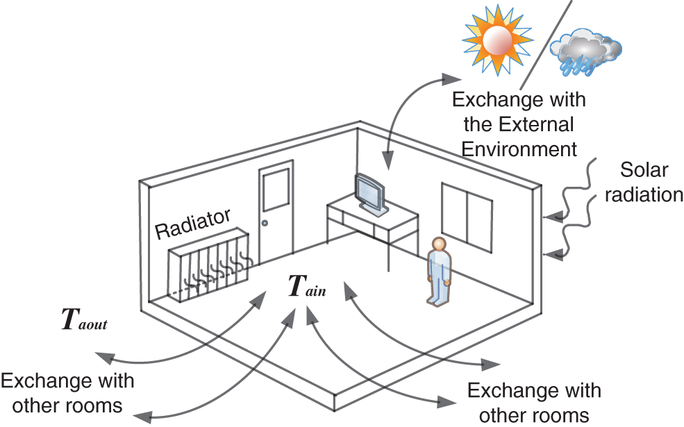
Figure 1: The representation of the heat balance inside a room

According to the description of the residential room for simulation in Section 2.1, the same heating method was adopted for the selected room and adjacent room. As the thermal environment of the room was consistent with that of the surrounding room, therefore, the heat conduction through the wall with the adjacent room and the heat penetration Qinf through the gap of the door were ignored, and only the heat conduction with the external environment was considered. The internal environmental thermal gain QiGain generated by indoor personnel and electronic equipment was negligible. Heat transfer from natural ventilation was also ignored. It was assumed that the radiator inlet temperature was constant, i.e., Trwin=Ct, and the backwater temperature varied with room temperature. Therefore, the simplified temperature dynamic equation of indoor heat conduction process was described by Eqs. (2)–(7),

maCaT˙ain=Qradiator+Qwindow+Qwall(2)

Qradiator=KradiatorAradiator(Tave−Tain)(3)

Qwindow=ISRAwindowgwindow+KwindowAwindow(Taout−Tain)(4)

Qwall=KwallAwall(Taout−Tain)(5)

0.58KvCwater(Trwin−Trwout)=KradiatorAradiator(Tave−Tain)+ρwaterVwaterCwaterT˙ave(6)

2Tave=Trwin+Trwout(7)

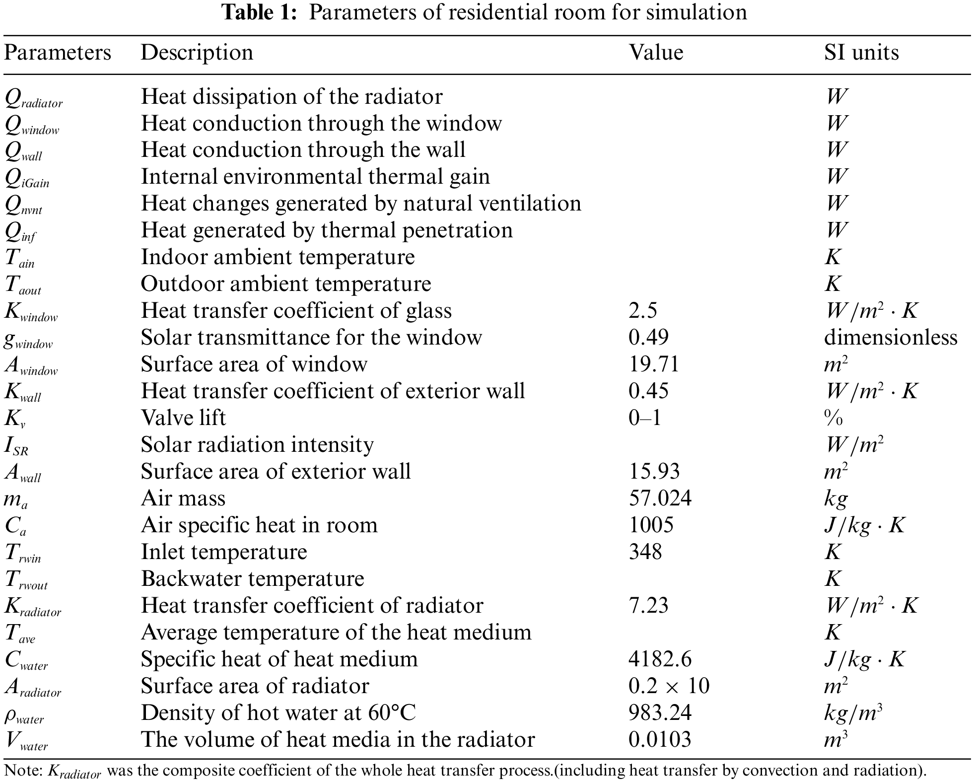
Eq. (6) was the temperature dynamic equilibrium equation of the radiator. The meanings of parameters in Eqs. (1)–(7) were shown in Table 1, the parameter values came from the design drawings of the heating room and relevant design code and standards [12,13].

Defined:

a=maCa; c=ρwaterVwaterCwater; d1=Awindowgwindow/a; d2=(KwindowAwindow+KwallAwall)/a;

b1=(KradiatorAradiator+KwindowAwindow+KwallAwall)/a; b2=KradiatorAradiator/a; b3=KradiatorAradiator/c; b4=Cwater/c.

Defined:

x=[Tain,Tave]T was the state variables of the system; yt=x1 was the output variables of the system;

ϑ=[ISR,Taout]T was the disturbing variable; u=Kv was the manipulated variables of the system.

The nonlinear temperature dynamic equation of indoor heat conduction process was described by Eq. (8),

{x˙=f(x,u,ϑ)yt=g(x,u)⇒{x˙1=−b1x1+b2x2+d1ϑ1+d2ϑ2x˙2=−b3(x2−x1)+1.16b4(Ct−x2)uyt=x1(8)

where, the elements in the x=[x1,x2]T vector were Tain and Tave, u was Kv, the elements in the ϑ=[ϑ1,ϑ2]T vector were ISR and Taout. It was necessary to consider the diameter of radiator electric valves and pipes, as well as the actual requirements for inlet and return water temperatures of the building heat network. So, the constraint set for the variable X was {x∈R2|278K⩽x1⩽308K,323K⩽x2⩽348K}; The constraint set for the variable U was U={u∈R2|0⩽u⩽1}.

2.3 Thermal Comfort

Generally speaking, the user's thermal comfort level in specific environment could be described by a function related to multiple environmental factors, including air quality of heating room, thermal comfort and visual comfort of residential users. In a certain environment, the thermal comfort of users was not only related to personal work efficiency, but also had a close relationship with people’s physical and mental health. Users' thermal comfort was influenced by physiological, physical and psychological processes, so it could be considered as a kind of human sensory and perceptual experience [14].

Thermal comfort was described as “the psychological state that people are satisfied with the surrounding thermal environment” in ASHRAE55-2017 [15,16]. Thus, it could be inferred from the definition that thermal comfort depended on a variety of environmental factors, such as the air temperature and relative humidity of heating room, air velocity in heating room and seasonal external climate. In addition, the research literature had demonstrated that people's choices of indoor air temperature were very similar when given the same thermal comfort conditions such as clothing, physical activity and climate, even if there were differences in the inhabited environment and culture of residential users around the world [14].

Therefore, an appropriate mathematical model could be used to calculate the thermal comfort level. The Predicted Mean Vote (PMV) index was one of the most common and widely used models, which expressed the thermal comfort level by the average thermal sensation of the residential users, and was proposed by Fanger in the 1970s [17]. Average thermal sensation was obtained by long-term prediction of residential users in different thermal environments based on the principle of energy balance of human body [18].

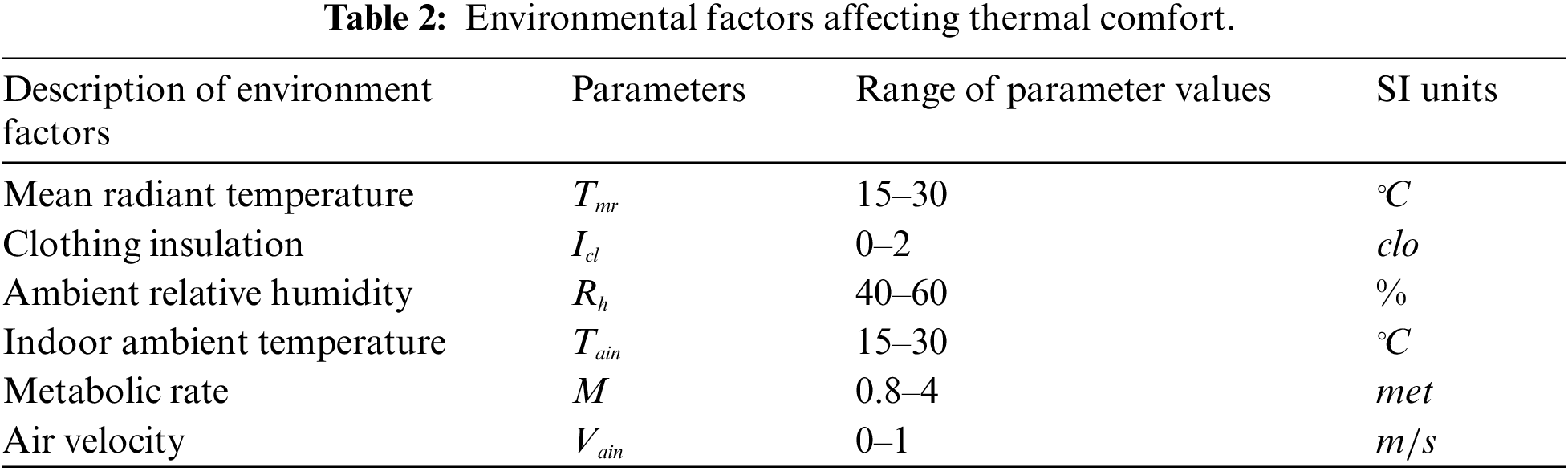
As can be seen from Table 2, PMV index is related to six factors, including M, Icl, Tain, Tmr, Vain and Rh [19]. Among them, mean radiant temperature, indoor ambient temperature, air velocity and ambient relative humidity could be measured [20]. Human metabolic rate and clothing insulation were not easy to calculate, because these two parameters depended on the location of the person in the room and the time of year, they could be obtained from manuals and international standards using look-up table method [14,17]. For example, the typical values of clothing insulation were 1.0 clo and 0.5 clo, respectively, in winter and summer (where, 1clo=0.155m2⋅∘C/W). In addition, the metabolic rate of human body could be selected to be equal to 1.0 met, in the typical indoor resting state of rest. The PMV index was calculated according to Eq. (9) [14],

PMV=[0.303e−0.036M+0.028]L(9)

In Eq. (9), M represented the metabolic rate of human body, and the unit was met. (1met=58.15W/m2, The parameter units identified later referred to the units used in the calculation of the formula). L represented the human thermal load, which was described as the difference between the heat generated inside the human body and the heat emitted by the human body in the actual environment under a certain thermal condition. This thermal load L could be calculated by Eq. (10),

L=(M−W)−0.0014M(34−Tain)−1.73×10−5M(5870−pa)−0.42(M−W−58.15)−3.96×10−8fcl[(Tcl+273)4−(Tmr+273)4]−3.05×10−3[5730−7(M−W)−pa]−fclhc(Tcl−Tain)(10)

Tain was the indoor ambient temperature, in unit of K, W was the mechanical work done by the human body in units of W/m2. pa represented the vapour pressure of water around human body, in unit Pa, which was related to the relative humidity of indoor air Rh and the vapour saturation pressure of water at Tain around the human body, and could be calculated by Eq. (11). Tmr represented the mean radiant temperature, in units of K. hc represented the convective heat transfer coefficient, in unit W/(m2⋅K). fcl represented clothing area coefficient, dimensionless. Tcl represented the surface temperature of clothing, in unit of K, which could be calculated by Eq. (12),

pa=Rhe(16.6536−4030.183Tain+235)(11)

Tcl=35.7−0.028(M−W)−0.155Icl{ fclhc(Tcl−Tain)+3.96×10−8fcl[ (Tcl+273)4−(Tmr+273)4 ] }(12)

hc and fcl in Eqs. (10) and (12) were calculated from Eqs. (13) and (14),

hc={2.38(Tcl−Tain)0.252.38(Tcl−Tain)0.25>12.1Vain12.1Vain2.38(Tcl−Tain)0.25<12.1Vain(13)

fcl={1.0+0.2IclIcl⩽0.5clo1.05+0.1IclIcl>0.5clo(14)

where, Icl represented the clothing insulation, in unit of clo. Vain represented the air velocity, in unit of m/s.

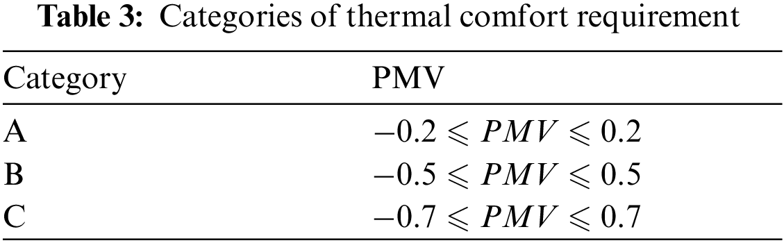
In conclusion, Eqs. (8) and (9) described the thermal comfort nonlinear model of the heating room. Table 3 showed the range of PMV parameters corresponding to three categories of thermal comfort requirements. According to literature [10], in the thermal comfort demand satisfaction survey, 90% of participants were satisfied with the thermal environment corresponding to thermal comfort category B. Therefore, the constraint set of thermal comfort index wasPMV={PMV∈R2|−0.5⩽PMV⩽0.5}.

3  Energy Efficient Thermal Comfort MPC(EETCMPC)

3.1 Control System Architecture

The primary purpose of the research was to present and design an energy efficient thermal comfort control strategy. Under this control strategy, users of green buildings could obtain an appropriate thermal comfort level, simultaneously, the economic cost of maintaining this thermal comfort environment could be optimized and reduced. Traditional MPC usually adopted hierarchical control structure to realize economic performance [9,21–23], that is, the upper layer was Real Time Optimization (RTO) layer, which obtained steady-state optimal set point through economic performance function, and the lower layer was control adjustment layer, which adopted MPC control strategy to realize set point tracking. However, this control structure ignored the economic performance of the whole dynamic process, and could only ensure that the system achieved economic optimization in the steady state set point. Economic Model Predictive Control (EMPC) was proposed in recent years, which integrated economic optimization and dynamic control regulation, and directly considered the economic efficiency during dynamic tracking, which could effectively improve the dynamic economic efficiency for control system. As shown in Fig. 2, The structure diagram of the EETCMPC system for heating rooms was presented in this study based on EMPC.

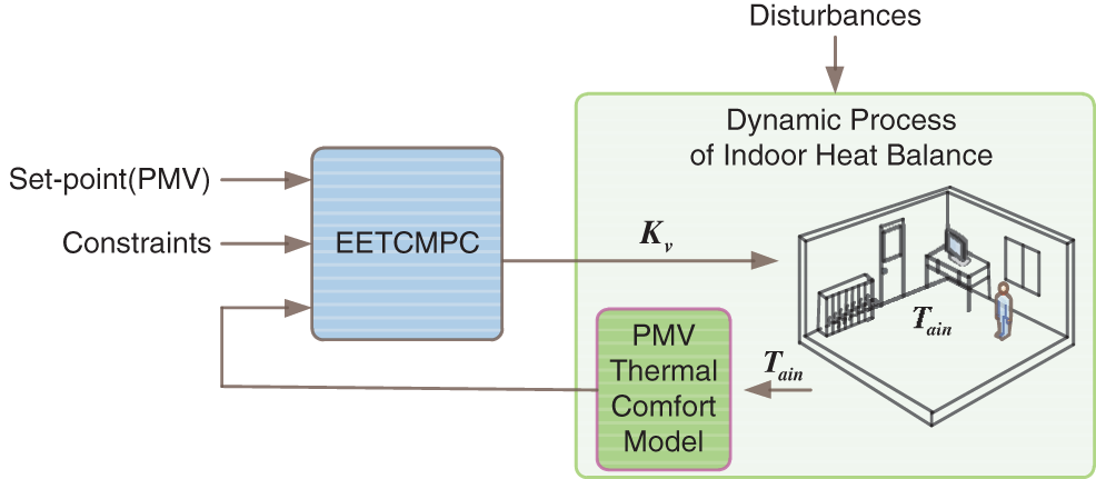
Figure 2: Control system architecture

3.2 A Nonlinear MPC Method

According to the nonlinear model given in Section 2, an approximate nonlinear prediction model was adopted in this study [24], as shown in Eq. (15),

Y~=f(Y←,u←,ϑ←,u)(15)

where the symbols were defined as follows:

Y← Historical and current values of thermal comfort PMV output.

u← Historical value of optimal manipulated variable (that is Kv).

ϑ← Historical values of measurable disturbances (that are ISR and Taout).

u=u0+δu=u(k−1)I+DΔu, where, I was the column vector of Nu×1 dimension, all elements were one, and Nu is the control horizon. Where, D was the lower triangular matrix of M×M dimension, and the elements were all one. Δu=[Δu(k)Δu(k+1)⋯Δu(k+Nu−1)]T.

Eq. (15) was transformed using first-order Taylor approximation expansion to obtain the following equation:

Y~=f(Y←,u←,ϑ←,u0)+∂Y~∂uδu(16)

From the symbol definition,

∂Y~∂uδu=∂Y~∂ΔuΔu(17)

Defined,

F=f(Y←,u←,ϑ←,u0),GNMPC=∂Y~∂Δu(18)

Then, Eq. (16) was transformed into the following equation:

Y~=F+GNMPCΔu(19)

where, F was the predicted output vector when Δu=0. Ny was the prediction horizon, GNMPC was the Jacobian of the predicted output Y~, and was obtained by Eq. (20),

GNMPC=[∂Y~k+1∂Δuk0⋯0∂Y~k+2∂Δuk∂Y~k+2∂Δuk+1⋯0⋮⋯⋯⋮∂Y~k+Ny∂Δuk∂Y~k+Ny∂Δuk+1⋯∂Y~k+Ny∂Δuk+Nu−1](20)

The calculation steps of GNMPC were as follows:

Step 1: Set Δu=[0,0,⋯,0]T, calculated F from Y←,u←,ϑ←, and obtained Y~0 vector, the length was the prediction horizon Ny, that was, Y~0=F.

Step 2: Calculated the first column of GNMPC, set a very small arbitrary value ε, such as ε=u(k−1)/1000, according to Step 1, set Δu=[ϵ,0,⋯,0]T and calculated Y~1 from Y←,u←,ϑ←, then GPNMPC(:,1)=(Y~1−Y~0)/ε.

Step 3: Calculated the second column of GNMPC, set Δu=[0,ϵ,⋯,0]T and calculated Y~2 from Y←,u←,ϑ←, then GPNMPC(:,2)=(Y~2−Y~0)/ε.

Step 4: Repeated Nu times, obtained Y~Nu, and finally get GPNMPC(:,Nu)=(Y~Nu−Y~0)/ε.

3.3 Economic Cost Function

Indicators such as thermal comfort index tracking and heat consumption could be considered in the economic cost function of indoor radiator heating systems and defined as the following equation:

{EIn1(y,u)=(PMV−y)2EIn2(y,u)=u(21)

where, PMV was the demand of thermal comfort index, EIn1 represented the tracking error of thermal comfort index, and EIn2 represented the heat consumption of heat medium in radiator. The economic benefit function of energy efficient thermal comfort could be obtained by linear weighting of thermal comfort index tracking and heat consumption,

EIn(y,u)=α1EIn1+α2EIn2(22)

where, α1,α2 were weight coefficients.

3.4 Optimization Problem

Based on the nonlinear prediction model and economic cost function mentioned above, the online optimization problem of EETCMPC was constructed as shown in Eq. (23),

minu(k+i|k)∑i=0Ny−1EIn(Y~(k+i|k),u(k+i|k))(23)

s.t.Y˜(k+i+1|k)=f(Y˜(k+i|k),u→(k+i−1|k),0)+GNMPCΔu(k+i|k)(24a)Y˜(k|k)=y(tk)(24b)umin⩽u(k+i|k)⩽umax(24c)Δumin⩽Δu(k+i|k)⩽Δumax(24d)i=0,1,⋯,Ny−1(24e)Y˜(k+N|k)=ys(24f)(24)

where, Ny represented the prediction horizon of EMPC, Y~(k+i|k) represented the predicted state of PMV at the future time, Eq. (24a) was the approximate nonlinear prediction model of room thermal comfort index at the current time tk (without considering interference). y(tk) was the actual system output at time tk, umin,umax were control constraints, Δumin,Δumax were control increment constraints. Eq. (24f) was the terminal equality constraint to ensure stability, ys was the optimal steady-state based on the economic cost function (22).

4  Results and Discussion

4.1 Simulation Data

In the simulation, the data of a certain sunny day in Zhengzhou (December 27, 2019) were selected from China Meteorological Data Network and obtained by linear interpolation. The outdoor temperature is given with green solid line and the solar radiation is given with purple solid line, as shown in Fig. 3. As described in Section 2.3, among the six factors that affect PMV index, mean radiant temperature, indoor ambient temperature, air velocity and ambient relative humidity were environmental factors that can be measured. In this study, indoor relative humidity and air velocity data were measured and obtained by hygrometer and thermal anemometer respectively, and stored in a one-day database, as shown in Fig. 4. There was little difference between the mean radiant temperature and the indoor ambient temperature. In simulation, the two were assumed to be equal and given by temperature dynamic model.

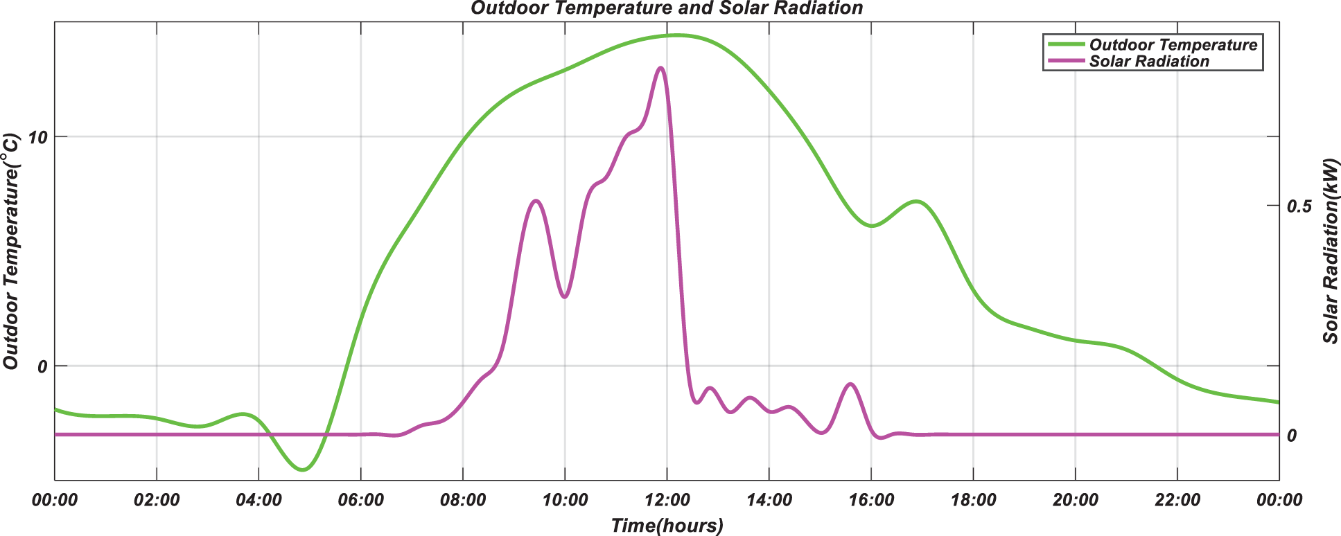
Figure 3: Outdoor climate data in Zhengzhou (December 27, 2019)

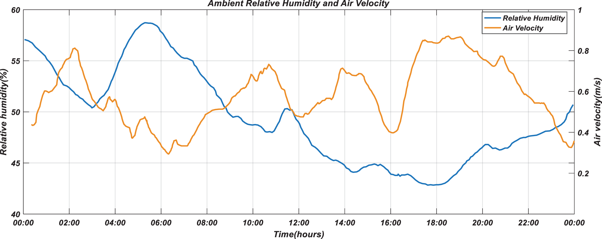
Figure 4: Relative humidity and air velocity data used for simulation

Human metabolic rate and clothing insulation were human factors that depend on the specific situation of the occupant. They were uncontrollable factors and should be selected according to the season, clothing and activity status of the occupant.

Under the calculation conditions M=1met, Vain=0.1m/s, Rh=50%, Tmr=Tain, Fig. 5 shows the curve of PMV changing with the clothing insulation at different temperatures. The calculated results show that PMV increases with the increase of clothing insulation at fixed temperature. From the slope, PMV increases greatly when the temperature is low, while PMV increases slightly when the temperature is high. In addition, when the clothing insulation is 0.5clo and the temperature range changes by 10∘C the PMV value changes by about 4. When the clothing insulation is 1.5clo and the temperature range changes by 10∘C, the PMV value changes by about 2. Thus, the higher the clothing insulation, the less the influence of temperature on PMV.

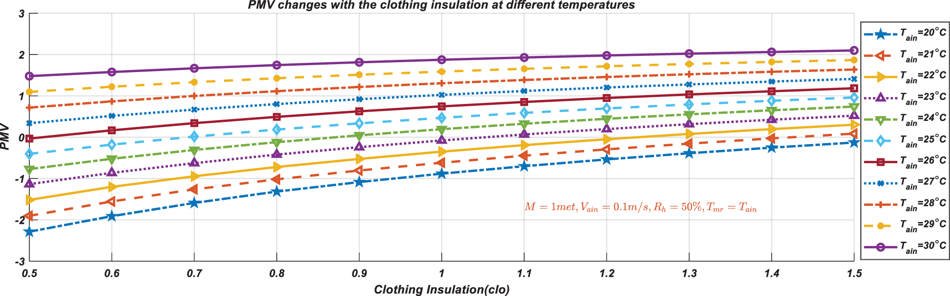
Figure 5: The curve of PMV changing with the clothing insulation at different temperatures

According to the residential room for simulation selected in this paper, in winter bedrooms, occupants were generally in a state of rest and wore sleepwear, which includes: Long-sleeve pajama tops, long pajama trousers, short 3/4 length robe (with slippers and socks). According to ANSI/ASHRAE Standard 55-2017, the clothing insulation value for a typical ensemble was 1 and the metabolic rate for a typical resting task was 1. When the clothing insulation was taken as a typical value, according to the PMV calculation Eq. (9) given in Section 2.3, under the calculation conditions M=1met, Icl=1clo, Vain=0.1m/s, Rh=50%, Tmr=Tain, the curve of PMV changing with temperature is shown in Fig. 6. As shown in the Fig. 6, when the indoor temperature ranges from 21.4∘C to 25.1∘C, satisfactory thermal comfort value of PMV can be obtained.

When the temperature changes, occupant adapted to the change by adding or removing clothes. Occupant's clothing was inversely proportional to temperature. The lower the temperature was, the greater the clothing insulation was required. The function of clothing insulation and temperature is shown in Fig. 7 [16].

Therefore, clothing insulation changed dynamically with temperature under the constraint of the function of clothing insulation and temperature. According to the PMV calculation Eq. (9) given in Section 2.3, under the calculation conditions M=1met, Vain=0.1m/s, Rh=50%, Tmr=Tain, the curve of PMV changing with temperature is shown in Fig. 8.

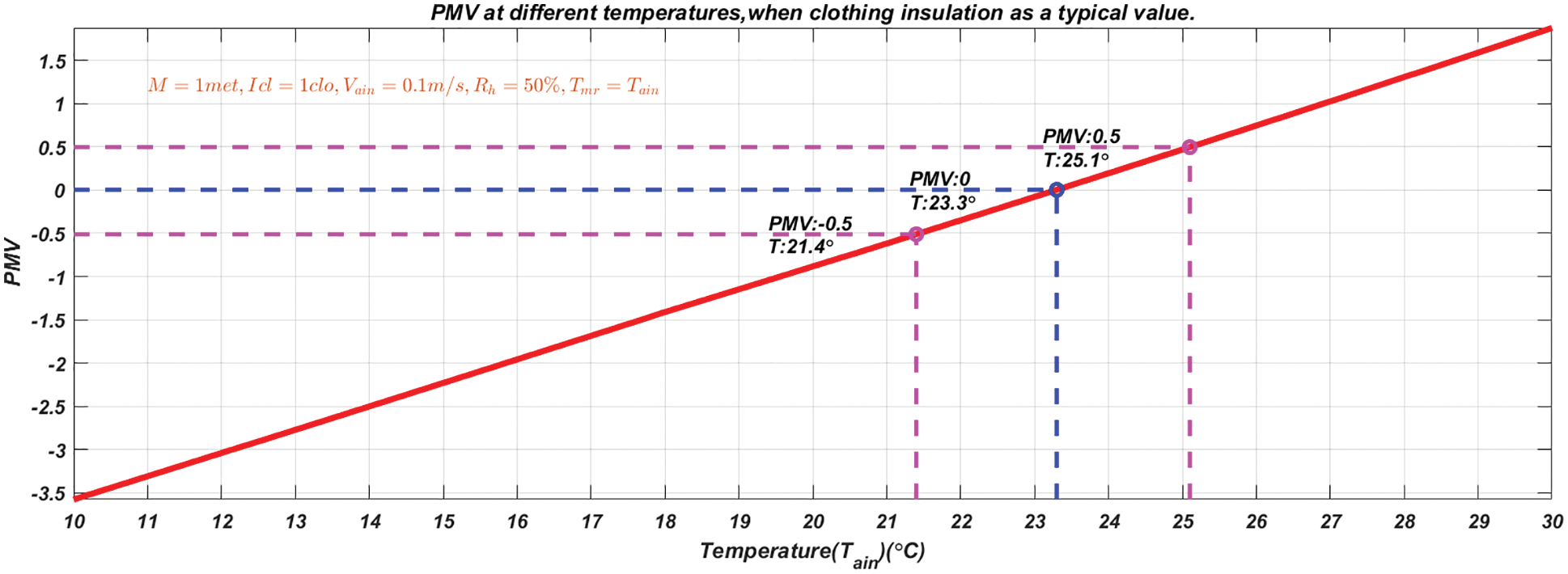
Figure 6: The curve of PMV with temperature when the clothing insulation is a typical value

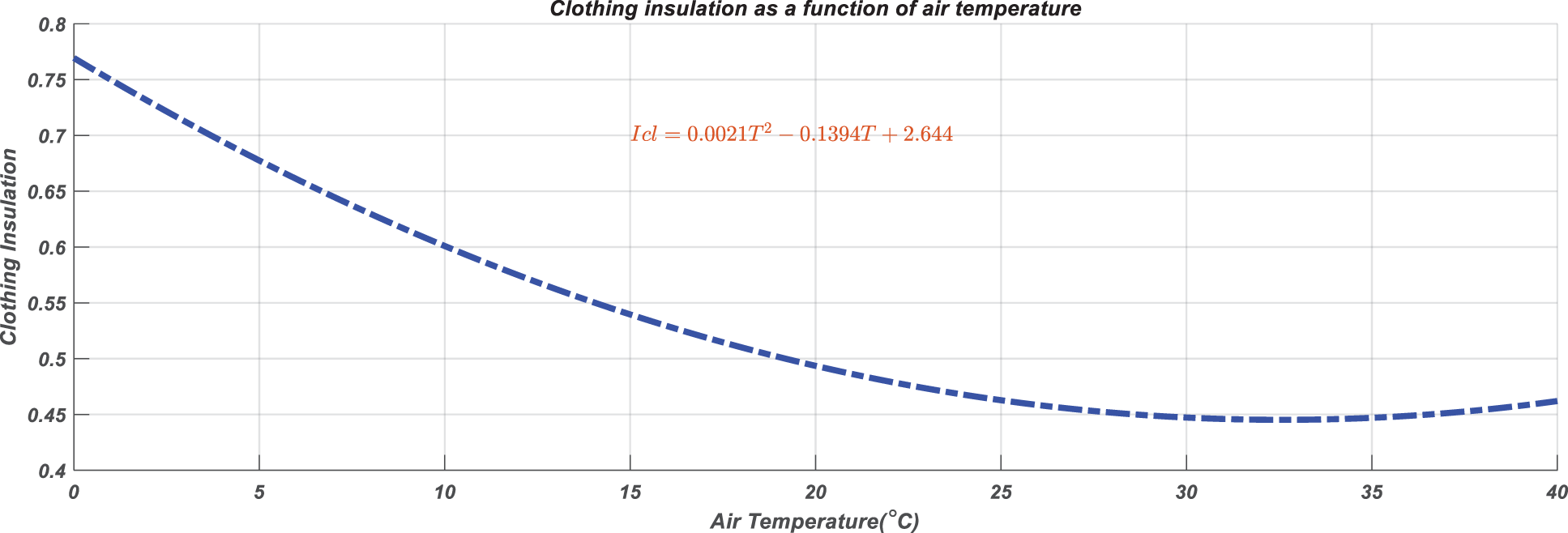
Figure 7: Clothing insulation as a function of air temperature

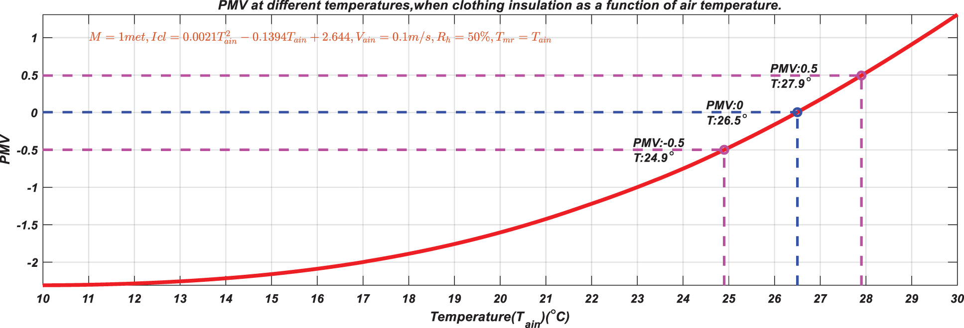
Figure 8: The curve of PMV with temperature when clothing insulation is a function of temperature

It can be seen from Figs. 5–8 that the clothing insulation has a great influence on PMV value. Therefore, the performance of the designed control strategy was analyzed when the clothing insulation was a typical value and the clothing insulation changed with temperature. The other simulation parameters are shown in Tables 1 and 2. All simulations were completed with MATLAB tools, and the running platform was a computer with a 2.9 GHz Intel I7 processor and 8 GB RAM memory.

4.2 Model Validation

Firstly, the approximate nonlinear model was verified. The process output is thermal comfort index (PMV), and the model inputs are manipulated variable Kv (valve lift) and disturbances (solar radiation ISR and outdoor ambient temperature Taout). Set Taout=5∘C(278K) and ISR=0.5kW/m2. When the indoor ambient temperature Tain=5∘C(278K), the PMV values calculated by the nonlinear model and its approximate model when Kv=20%,50%,80%, as well as the errors between the two models are given, respectively, as shown in Fig. 9. When Kv=50%, the PMV values calculated by the nonlinear model and its approximate model when Tain=5∘C(278K),10∘C(283K),15∘C(288K), as well as the errors between the two models are given respectively, as shown in Fig. 10. It can be seen from Figs. 9 and 10 that the approximate nonlinear model obtained approximates properties of the process very well.

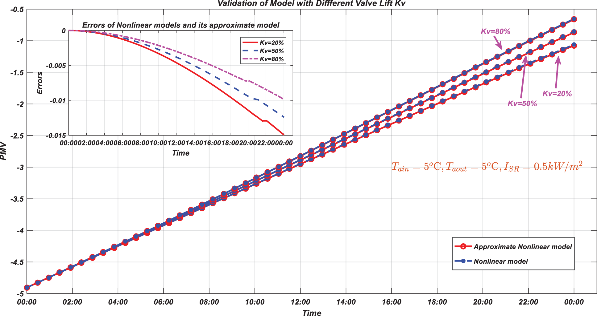
Figure 9: Nonlinear model vs. its approximate model with different Kv

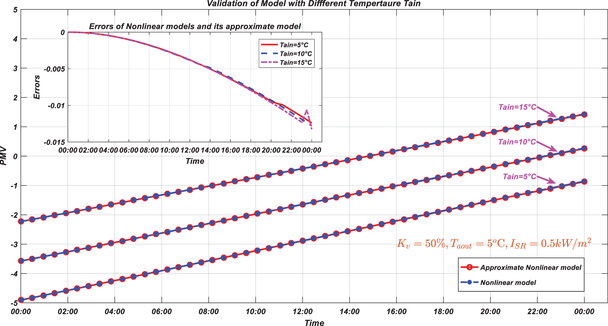
Figure 10: Nonlinear model vs. its approximate model with different Tain

4.3 Simulation Scenario 1: PMV with Step Change

With the view of validating the performance of the EETCMPC constructed in this study, a simulation comparison was made with the traditional Double-Layer Model Predictive Control (DMPC). The control horizon Nu=3 and the prediction horizon Ny=20. In the DMPC structure, the Steady-State Target Optimisation (SSTO) objective optimization method proposed in literature [9] was adopted in the RTO layer to calculate and obtain the optimal steady-state temperature set point, which was sent to the MPC of the regulation layer to complete the set point tracking.

According to the selected variation range of PMV, the initial thermal comfort index was selected as 0. For the purpose of verifying the validity of the control strategy, it was assumed that the heating room was in a state of heat balance during the 0:00–2:00, and the input value of the thermal comfort index stepped to 0.5 at 2:00. Figs. 11–13 show the temperature, thermal comfort index and valve lift curves of the heating room under EETCMPC and DMPC control strategies.

The optimal steady-state temperature set point obtained by RTO is given by the solid red line in Fig. 11, corresponding to the thermal comfort index with step change in DMPC. The room temperature under the EETCMPC is given by the solid blue line in Fig. 11 and calculated from the simulation results of PMV in Fig. 12.

Figure 11: Simulation results for temperature (simulation scenario 1)

Fig. 12 shows that the output response time of the system under the action of EETCMPC is larger than that of DMPC because EMPC sacrifices some tracking performance to improve the economy in dynamic process. Fig. 9 shows that the lift of the radiator inlet valve decreases so the heat medium flow into the radiator is decreased, that is, more heat is no longer needed to achieve the temperature tracking target, but only a certain amount of heat is radiated to ensure the thermal comfort level in the room during the dynamic response process under the action of EETCMPC. Therefore, the energy required for heating is also reduced and the economic performance is improved.

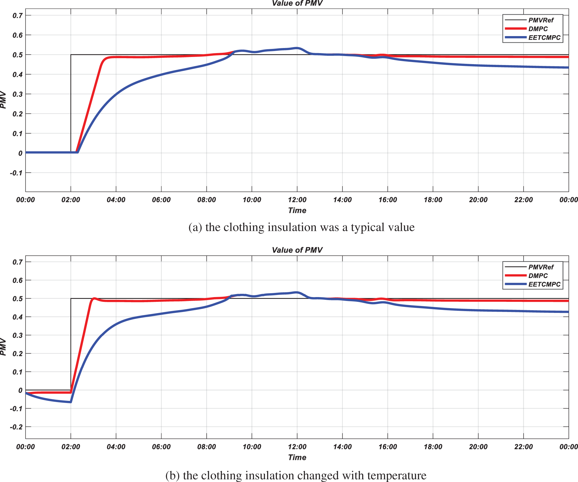
Figure 12: Simulation results for PMV (simulation scenario 1)

As shown in Fig. 13, except for the step phase, a certain amount of heat to maintain temperature balance is radiated from the radiator under the controller during the night. The temperature of the room is raised by outdoor disturbances in natural means such as conduction, convection and radiation during the day. In this case, the valve lift is reduced by the controller, and then, the heat dissipation of the radiator is decreased with the view of reducing energy cost. The influence of outdoor disturbance can be observed from Fig. 13, and the control signal curve has obvious fluctuation during 9:00–13:00. It can be seen from Fig. 3 that the solar radiation during 07:00–13:00 is one of the main reasons for this fluctuation. The influence of this disturbance on the thermal comfort of heating room can be effectively eliminated under the two control strategies of EETCMPC and DMPC.

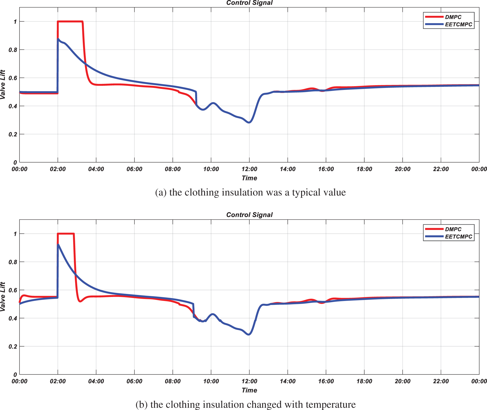
Figure 13: Simulation results for control signal (simulation scenario 1)

4.4 Simulation Scenario 2: PMV Varies with Demand

The actual heat demand in the heating system was affected by non-human factors and human factors. Non-human factors were mainly the disturbance of the ambient conditions, and the influence caused by the disturbance could be eliminated by the controller, which was described in the simulation scenario 1. For human factors, such as the time of work and rest, at night, people mainly slept on the bed, considering the existence of quilt, heat demand could be minimized; During the day, people were mainly in the state of work and leisure, and the demand for heat was higher. Therefore, the thermal comfort index from 10:00 to 06:00 was set as –0.5, and the heat demand was the lowest. The thermal comfort index of the two periods of 6:00–11:00 and 17:00–22:00 was set as 0.5, and the heat demand was the highest (during this period, the external temperature was relatively low). The thermal comfort index from 11:00 to 17:00 was set as 0, and the heat demand was normal (during this period, the outside temperature was relatively high). Simulation was used to illustrate the effect of the EETCMPC in the dynamic process, and the simulation parameters were set in accordance with simulation scenario 1. Figs. 14–16 show the temperature, thermal comfort index and valve lift curves of the heating room when the heat demand changes under EETCMPC and DMPC control strategies.

The optimal steady-state temperature set point obtained by RTO is given by the solid red line in Fig. 14, corresponding to the thermal comfort index changes with the heat demand in DMPC. Compared with the room temperature under the EETCMPC strategy (solid blue line), it varies in a larger range and requires more energy to maintain the temperature within a larger range. The indoor thermal comfort index is stabilized at the set point under the EETCMPC and DMPC strategy, when the PMV set point changes with the heat demand, as shown in Fig. 15. When the heat demand changes (06:00, 11:30, 17:00, 22:00), economy is the main objective of controller optimization under EETCMPC. The response time of system output under EETCMPC is larger than that of traditional DMPC. At the same time, it can be seen from Fig. 16 that the valve lift decreases during the dynamic response process under the EETCMP controller, so the heating consumption decreases and the economic performance improves.

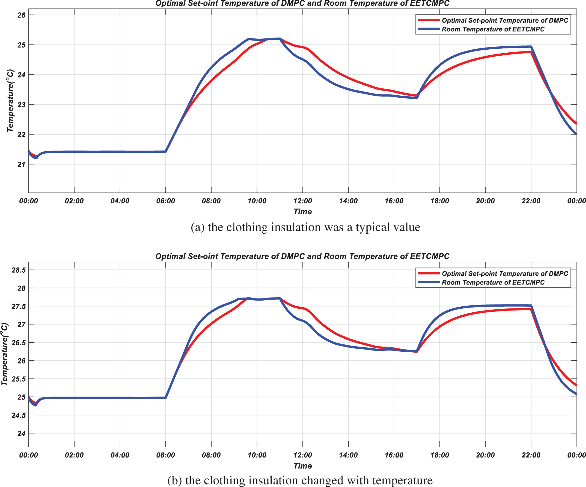
Figure 14: Simulation results for temperature (simulation scenario 2)

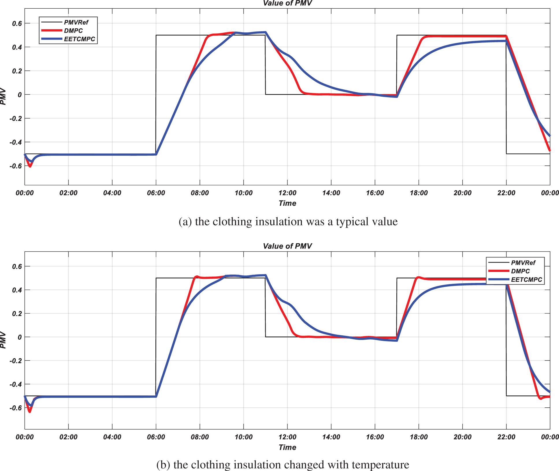
Figure 15: Simulation results for PMV (simulation scenario 2)

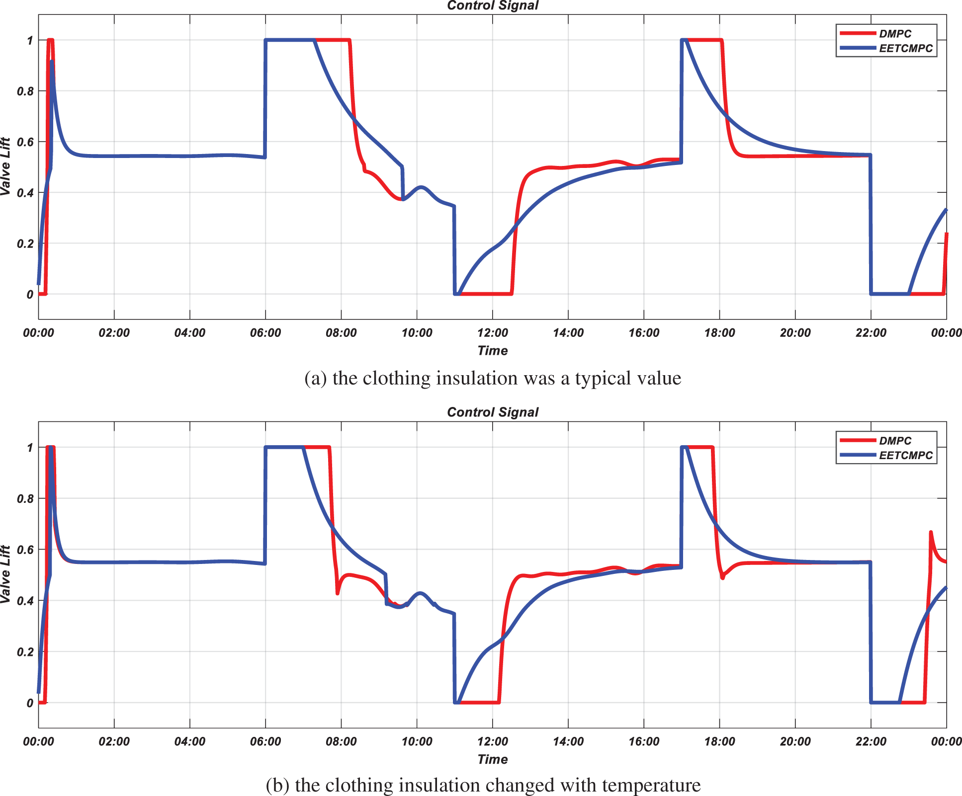
Figure 16: Simulation results for control signal (simulation scenario 2)

4.5 Analysis of Economic Performance

The variation trajectories of cost function EIn in simulation scenario 1 and simulation scenario 2 are shown in Figs. 17 and 18. It can be seen from Fig. 17 that, in simulation scenario 1, the steady-state economic optimal points of the two control strategies are basically the same, and economic cost tend to the steady-state optimal point, indicating that the two control strategies can reach the economic optimal point when PMV changes with step. During 2:00–11:00 (PMV step change), the value of the blue curve is smaller than that of the red curve, and the stabilization time is faster than that of the red curve, indicating that the economic performance of EETCMPC is better than that of DMPC in the dynamic process. During 19:00 to 00:00, the red curve gradually deviates from the steady-state optimum, indicating that the economic performance of DMPC begins to deteriorate. As shown in Fig. 18, in simulation scenario 2, when PMV changes with heat demand, the economic cost of the two control strategies change with time and both of them tend to their own steady-state economic optimal point. However, the steady-state economic optimal point under the EETCMPC control strategy is less than that under the DMPC, indicating that the global economic optimal point can be achieved under the EETCMPC control strategy, while the DMPC can only reach its optimal steady-state set point. According to (a) and (b) of Fig. 18, when the clothing insulation changes with temperature, the steady-state economic optimal point of the two control strategies does not differ much. However, under the EETCMPC control strategy, when the clothing insulation of clothing changes with temperature, the steady-state economic optimal point is larger than that when the clothing insulation is typical value, indicating that the change of clothing insulation affects the steady-state economic optimal point of the controller. This is caused by the coupling relationship between the thermal resistance of clothing and temperature in the model.

To evaluate the energy efficient effect of control strategies, the total radiant heat of radiators under different control strategies during the simulation period [tstart,tend] could be calculated from Eq. (25),

Eradiator=∫tstarttend0.58KvCwater(Trwin−Trwout)dt(25)

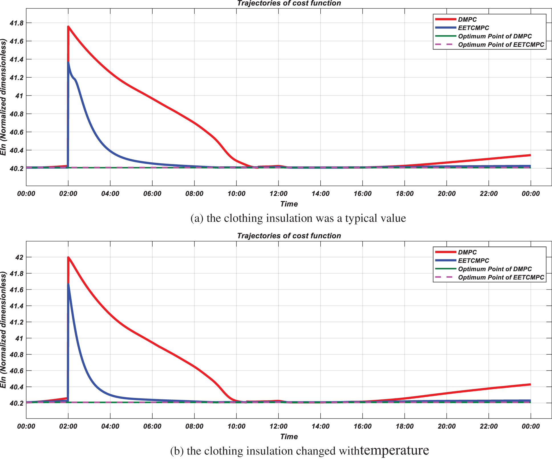
Figure 17: Trajectories of economic cost function (simulation scenario 1)

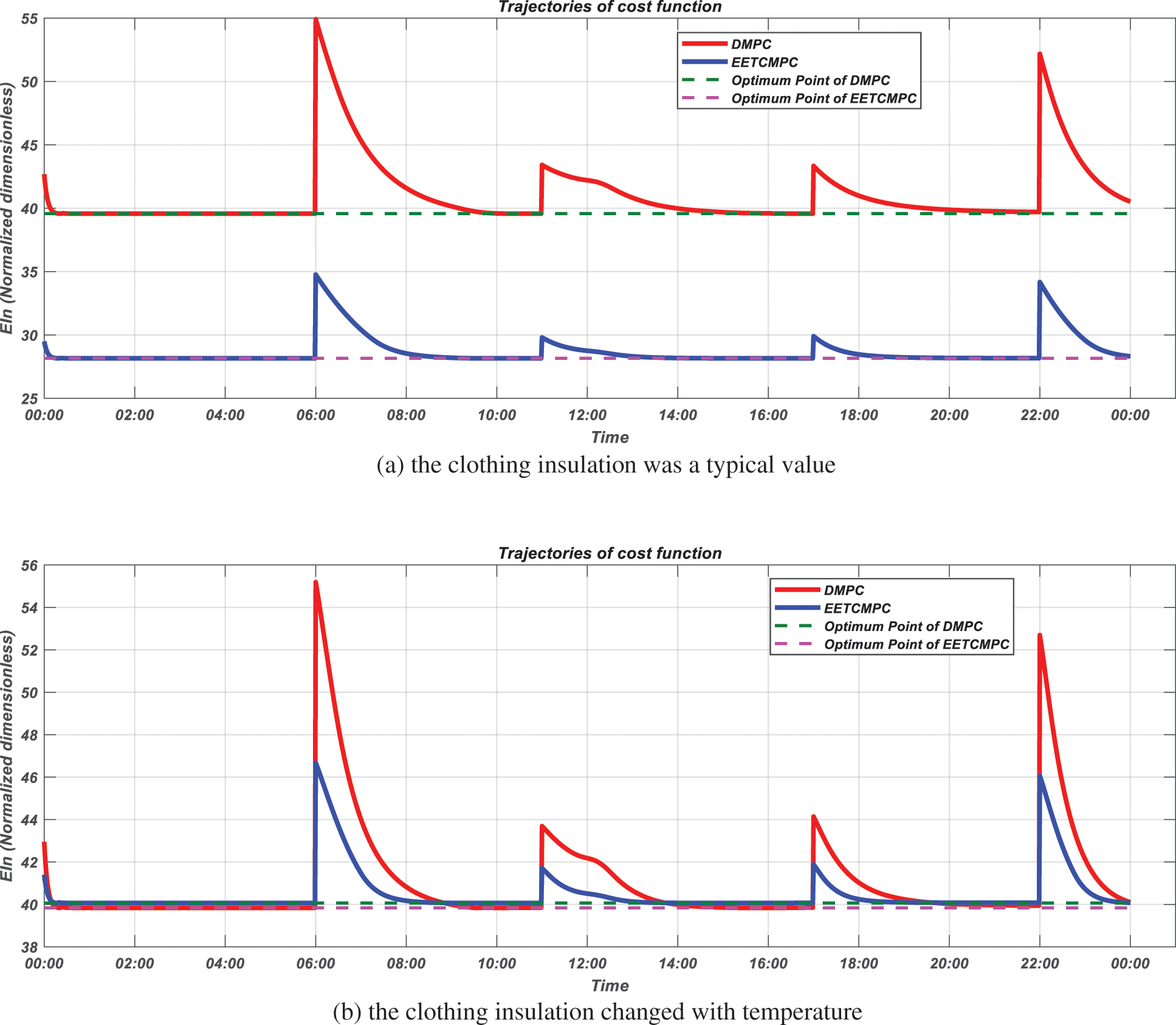
Figure 18: Trajectories of economic cost function (simulation scenario 2)

The energy consumptions of EETCMPC and DMPC control strategies in the two simulation scenarios are shown in Fig. 19.

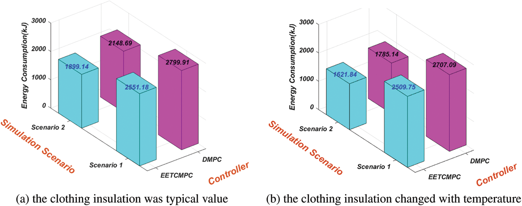
Figure 19: Comparison of energy consumptions

When the clothing insulation was typical value, in simulation scenario 1, the energy consumption of EETCMPC was reduced by 8.9% compared to DMPC, resulting in a lower economic cost. In simulation scenario 2, the energy consumption of both control strategies was lower than that of simulation scenario 1, because the heat demand was reduced according to the schedule. Compared with DMPC, the energy consumption of EETCMPC was reduced by 11.6%, which further reduced the economic cost, indicating that the economic performance was further improved.

When the clothing insulation changed with temperature, the energy consumption of EETCMPC was reduced by 7.29% and 9.15% compared with that of DMPC in simulation scenario 1 and simulation scenario 2, respectively. Compared with the typical clothing insulation, the range of energy efficient was reduced. However, the total energy consumption was decreased. Under the EETCMPC control strategy, the reduction was about 14.6% in simulation scenario 2 and 1.65% in simulation scenario 1, which indicates that the total energy consumption was reduced and the economic performance was further improved under the two control strategies when the clothing insulation changed with temperature.

5  Conclusions and Future Works

The nonlinear model of thermal comfort for the heating room of household control and thermal metering building was firstly presented, and a practical approximate nonlinear thermal comfort prediction model was established. The economic benefit function was designed. In order to reduce the heat radiation from the radiator in the process of PMV tracking and improve the economic performance, an EETCMPC strategy was constructed. Simulation results showed that the EETCMPC strategy achieved economic cost optimization of dynamic process and has energy efficient effect. Therefore, the EETCMPC control strategy could be applied to green building heating system to reduce the economic cost of heating under thermal comfort conditions.

In future works, one of the interest directions of future research is the optimization of heating cost considering the change of heating price (peak and valley thermal charges) and weather forecasts.

Funding Statement: This work was supported by the Key Technologies R&D Program of Henan Province (Nos. 202102210335/212102210026/212102210509/222102220095/212102110218), the Key Scientific and Technological Project (Social Development Field) of Henan Province, China (No. 212102310093), the Key Scientific Research Projects of Institutions of Higher Education in Henan Province (No. 20B413007) and the Science and Technology Program of Henan Province Department of Housing and Urban Rural Construction (No. K-1916).

Conflicts of Interest: The authors declare that they have no conflicts of interest to report regarding the present study.

References

 1.  China Association of Building Energy Efficiency (2019). China building energy consumption research report 2018. Construction and Architecture, 2, 26–31 (in Chinese). [Google Scholar]

 2.  Henan Provincial People's Congress Standing Committee (2017). Regulations of Henan Province on energy conservation. Zhengzhou, China: Henan Daily Press. [Google Scholar]

 3.  Kajgaard, M. U., Mogensen, J., Wittendorff, A., Veress, A. T., Biegel, B. (2013). Model predictive control of domestic heat pump. American Control Conference, Washington DC, USA. [Google Scholar]

 4.  Vašak, M., Martinčević, A. (2013). Optimal control of a family house heating system. 2013 36th International Convention on Information and Communication Technology, Electronics and Microelectronics (MIPRO), Opatija, Croatia [Google Scholar]

 5.  Kurilla, J., Hubinsky, P. (2017). Model predictive control of room temperature with disturbance compensation. Journal of Electrical Engineering, 68(4), 312–317. DOI 10.1515/jee-2017-0044. [Google Scholar] [CrossRef]

 6.  Suda, T., Namerikawa, T. (2018). Robust prediction and MPC-based optimal energy management for HVAC System. IFAC-PapersOnLine, 51(25), 472–477. DOI 10.1016/j.ifacol.2018.11.182. [Google Scholar] [CrossRef]

 7.  Yang, S., Wan, M. P., Chen, W., Ng, B. F., Zhai, D. (2019). An adaptive robust model predictive control for indoor climate optimization and uncertainties handling in buildings. Building and Environment, 163(1), 106326. DOI 10.1016/j.buildenv.2019.106326. [Google Scholar] [CrossRef]

 8.  Barata, F. A., Neves-Silva, R. (2012). Distributed model predictive control for thermal house comfort with auction of available energy. International Conference on Smart Grid Technology, Economics and Policies (SG-TEP), Nuremberg, Germany. [Google Scholar]

 9.  Ławryńczuk, M., Ocłoń, P. (2019). Model predictive control and energy optimisation in residential building with electric underfloor heating system. Energy, 182, 1028–1044. DOI 10.1016/j.energy.2019.06.062. [Google Scholar] [CrossRef]

10. Sian En, O., Yoshiki, M., Lim, Y., Tan, Y. (2018). Predictive thermal comfort control for cyber-physical home systems. 2018 13th Annual Conference on System of Systems Engineering (SoSE), Paris, France. [Google Scholar]

11. Yaser, A., María, C., José, Á., Antonio, R. (2017). An economic model-based predictive control to manage the users’ thermal comfort in a building. Energies, 10(3), 1–18. DOI 10.3390/en10030321. [Google Scholar] [CrossRef]

12. Ministry of Housing and Urban-Rural Development of the People's Republic of China (2012). Design code for heating ventilation and air conditioning of civil buildings. Beijing: China Architecture & Building Press. [Google Scholar]

13. Henan Province Department of Housing and Urban Rural Construction (2017). Henan Province design standard for energy efficiency of residential buildings (cold zone 75%). Zhengzhou: Zhengzhou University Press. [Google Scholar]

14. ASHRAE (2017). ASHRAE handbook—Fundamentals. Atlanta, GA, USA: Refrigerating American Society of Heating and Air-Conditioning Engineers. [Google Scholar]

15. Fanger, P. O. (1973). Assessment of man's thermal comfort in practice. British Journal of Industrial Medicine, 30(4), 313–324. DOI 10.1136/oem.30.4.313. [Google Scholar] [CrossRef]

16. ASHRAE (2017). Ansi/ashrae standard 55-2017: Thermal environmental conditions for human occupancy. Atlanta, GA, USA: American Society of Heating, Refrigerating and Air Conditioning Engineers. [Google Scholar]

17. Fanger, P. O. (1972). Thermal comfort analysis and applications in environment engineering. NewYork, USA: McGraw-Hill. [Google Scholar]

18. Orosa, J. A. (2009). Research on general thermal comfort models. European Journal of Scientific Research, 27(2), 217–227. [Google Scholar]

19. Hong, S. H., Lee, J. M., Moon, J. W., Lee, K. H. (2018). Thermal comfort, energy and cost impacts of PMV control considering individual metabolic rate variations in residential building. Energies, 11(7), 1767. DOI 10.3390/en11071767. [Google Scholar] [CrossRef]

20. Tse, W. L., Chan, W. L. (2007). Real-time measurement of thermal comfort by using an open networking technology. Measurement, 40(6), 654–664. DOI 10.1016/j.measurement.2006.07.005. [Google Scholar] [CrossRef]

21. Ma, J., Qin, S. J., Salsbury, T. (2014). Application of economic MPC to the energy and demand minimization of a commercial building. Journal of Process Control, 24(8), 1282–1291. DOI 10.1016/j.jprocont.2014.06.011. [Google Scholar] [CrossRef]

22. Staino, A., Nagpal, H., Basu, B. (2016). Cooperative optimization of building energy systems in an economic model predictive control framework. Energy & Buildings, 128(2), 713–722. DOI 10.1016/j.enbuild.2016.07.009. [Google Scholar] [CrossRef]

23. Kuboth, S., Heberle, F., König-Haagen, A., Brüggemann, D. (2019). Economic model predictive control of combined thermal and electric residential building energy systems. Applied Energy, 240(9), 372–385. DOI 10.1016/j.apenergy.2019.01.097. [Google Scholar] [CrossRef]

24. Castilla, M., Álvarez, J. D., Normey-Rico, J. E., Rodríguez, F. (2014). Thermal comfort control using a non-linear MPC strategy: A real case of study in a bioclimatic building. Journal of Process Control, 24(6), 703–713. DOI 10.1016/j.jprocont.2013.08.009. [Google Scholar] [CrossRef]

This work is licensed under a Creative Commons Attribution 4.0 International License, which permits unrestricted use, distribution, and reproduction in any medium, provided the original work is properly cited.