Energy Engineering

---

DOI: 10.32604/ee.2022.021342

ARTICLE

Optimal Intelligence Planning of Wind Power Plants and Power System Storage Devices in Power Station Unit Commitment Based

Yuchen Hao*, Dawei Su and Zhen Lei

Control Center of State Grid of Jiangsu Electric Power Co., Ltd., Nanjing, 210000, China
*Corresponding Author: Yuchen Hao. Email: yuchenhao2021@163.com
Received: 10 January 2022; Accepted: 15 March 2022

Nomenclatures

Pit	Generated power of generator i at time t
Δ1t	Load uncertainty budget
Pwt	Generated power of wind farm w at time t
Δ2t	Wind farm-generated power uncertainty budget
SnP	Generated power of ESS r at time t
YrBegin	Initial energy of ESS r
Srts	Consumed power of ESS r at time t
YrLast	Final energy of ESS r
Yr,t	Capacity of ESS r at time t
t	Time
PL1	Power passing line l
n	Bus
Xit	Presence or absence of generator i at time t
j	Busbar
Uit	Generator i turning on at time t
w	Wind farm
Vit	Generator i turning off at time t
r	ESS
Sit	Cost of commissioning
i	Non-wind power station
Git	OFF cost
1	Transfer line
Cit	Cost per MWH of electricity generated by the non-wind power station
U(n)	Set of units in bus n
Crp	Cost per MWH of ESS discharging
W(n)	Set of wind farms in bus n
Crs	Cost per MWH of ESS charging
R(n)	Set of ESS in bus n
MinUPi	Minimum ON time
MinDWi	Minimum OFF time
J(n)	Set of loads in bus n
RDit	Decreasing slope rate
N(w)	Set of wind farms with wind uncertainty
RUit	Increasing slope rate
N(d)	Set of unit loads with uncertainty
pimin	Minimum power generated by each non-wind power station
Δ1t	Load uncertainty budget
pimax	Maximum power generated by each non-wind power station
Δ2t	Wind farm-generated power uncertainty budget
PLimax	Maximum power passing the line
YrBegin	Initial energy of ESS r
djt	Load in bus j at time t
YrLast	Final energy of ESS r
SrminS	Minimum ESS charging power
t	Time
SrmaxP	Minimum ESS discharging power
n	Bus
SrmaxS	Maximum discharging power
j	Busbar
Yrmin	Minimum ESS capacity
w	Wind farm
Yrmax	Maximum ESS capacity
ηs	ESS charging efficiency
ηp	ESS discharging efficiency

1  Introduction

Reduction of system operating costs is a critical economic program in power systems. As such, programming for unit commissioning and decommissioning is of utmost importance. Generally, two objectives of “ensuring safe operation” and “facilitating economic operation” are of significance. The unit commissioning/decommissioning problem was designed and implemented based on the grid's security principles in the traditional power system operation. In this case, grid operation was not necessarily the most economical mode of operation. In the restructured environment, security can be facilitated by using various services available to the market and the electricity consumption price can be reduced by the economic use of the electricity market [1].

Due to uncertainties related to the load prediction error, unexpected generator decommissioning, and transfer line outages during real-time operation, operators have to deviate from the pre-determined decisions by the unit commitment (UC) program and take costly modification measures, e.g., rapid generator commissioning or load disconnection to maintain system security [2]. The rising fossil fuel prices, their limited supply, and their resulting pollution, clarify the necessity of replacing them with new and clean energy sources. Solar energy systems are a major RES due to their availability, low maintenance costs, lack of mobile components, bio-friendliness and longevity. The increased penetration of RESs that have fluctuating power generation, e.g., solar and wind energy, introduces more uncertainty to the system and poses new challenges for the grid manager and generation programming. There is a dire need for a UC process to manage system uncertainty [3]. Currently, the electricity generation industry uses reserve constraints for the UC problem to deal with uncertainty. Reserve requirements are often highly conservative, making it economically inefficient. Moreover, standards for determining reserve levels are based on the expected demand. This means that the solution for the UC problem with reserve constraints may not supply the demand in real time due to the serious deviation from the prediction demand [4].

Due to the uncertainty in dispersed energy sources, the existence of an energy storage system (ESS) beside the RES is an efficient solution to attaining a proper level of confidence. In regular low-voltage grids, ESSs are mainly employed by the end-users for peak shaving or protection against short-term breaks in resources. With the emergence of MGs and the development of ESSs, the role of this equipment has become more and more prominent. As an ESS, DG sources such as wind farms generate fluctuating loads due to the variable nature of wind [5]. These fluctuations negatively affect the power quality, voltage, and system frequency. The use of ESSs along with photovoltaic (PV) and wind farms can make this variable output power more uniform. To this end, various ESS technologies and their connecting methods have been proposed. A very popular method for dealing with power system uncertainty is stochastic programming. Different studies on power station UC and uncertainty are reviewed below [6].

In [7], a robust two-stage optimization model was introduced to solve UC problems by considering variable wind power generation. In [8], a robust optimization approach was proposed to adapt to wind output uncertainty. In [9], the difference between multi-band robust optimization and Seng-Cheol robust optimization was analyzed. This study also improved the multi-band robust optimization parameter setting method based on the wind power sample. The results were tested on an IEEE 39-bus power system with three wind farms. In [10], UC scheduling on integrated fuel and natural gas systems was examined. Natural gas storage in the gas network support problem was done during peak hours via reducing pipeline congestion. A hydrogen energy storage system was integrated with novel flexible technologies, including power-to-gas (P2G) and demand response program (DRP), in order to reduce the RES costs of operation and transfer the peak load demand to peak hours. In [11], a sensitivity analysis was performed to evaluate the effect of increasing thermal load on the combined heat and power (CHP) unit operation as its thermal and electrical output. A plug-in electric vehicle (PEV) charging station was integrated with this problem to examine its effects on grid performance since PEVs introduced an unplanned and undetermined load to this system. In [12], the advantages of combining the stochastic programming framework with reserve constraints were examined.

In [13], water reserve pump units were used to control the uncertainty of wind units based on the robust optimization in the UC problem. In [14], a general ESS, i.e., any device storing and transferring energy, was utilized. Several simplifying assumptions were included for the ideal ESS in its technical and economic performance. In [15], the use of electric energy storage systems as a proper strategy was introduced for reducing fluctuations and using renewable dispersed generators in the MG. In [16], uncertainties were dealt with by vastly adopting two-stage robust optimization methods for power system operations and programming problems. In [17], the large-scale wind power integration problem and the significant challenges it causes for the safe and economic performance of the power system were dealt with. To tackle wind power uncertainty, this paper proposed a two-stage stochastic UC model, in which the wind power prediction error was described via the mixed multi-dimensional Gaussian model. In [18], the unit programming problem was examined in the presence of wind farms and a power system storage system. In [19], a modified formula was presented for the battery-thermal UC problem that combined BESS with thermal units to compensate for wind power generation uncertainty. In [20], the commitment of a hydrogen storage system and DR was dealt with to mitigate the problems related to wind power integration in the system.

In [21], an optimality decomposition algorithm is used to solve security-constrained OPF problem in present of wind power is proposed. In order to reduce the calculation time, in process state a filtering approach is applied to the algorithm. The proposed strategy is applied in different load, generation and network configurations scenarios to illustrate the proposed strategy in this paper. Using power system dividing approach for unit commitment model in present of wind turbines to achieve reliable, secure and optimal generation units is proposed in [22]. Uncertainties in wind generations and load prediction are considered in this model. For reliability study, a powerful intelligence method is applied. In [23], an optimal dynamic economic emission dispatch problem model is proposed in present of wind turbine, electric vehicles, thermal electric generation is proposed to minimize cost and emission of system. This paper is model the problem based on nonlinear problem and optimized with new fuzzy based optimization model. In [24], an optimal market-based model based on system of system concept for the secure and economic hourly generations is proposed. decentralized modelling, uncertainty considering, prediction model, scenario reduction and security constrains considering are the main contributions of this paper. Also, another decentralized model for R-SCUC problem is proposed in [25]. In this model the uncertain model is modeled by probability distribution function and weibull probability distribution for load and wind predictions, respectively.

The present study solved the security-constrained UC problem in the presence of wind farms and ESS having load and wind-generated power uncertainties via a novel optimization method. The grid load and power generated by the wind farms were included in the problem as uncertainties. Our proposed method aimed to present UC programming for the previous-day market that minimized the total costs under the worst-case scenario of uncertainty in real time. The main novelties of the proposed strategy could be written as follows:

✓   New model strategy defining for UC problem in modern power systems containing undispatchable power resources and storage system;

✓   Uncurtains factors modelling of undispatchable power resource in present UC problem using PDF;

✓   Adopted a novel method to perform security-constrained UC programming in the presence of a wind farm and ESS with load and wind farm-generated power uncertainty;

✓   Minimizing grid operation cost for worst load condition of system;

✓   Applying two stage optimization algorithms to reach the global best solution of the UC problem.

2  Problem Model

2.1 Deterministic Model

The deterministic model of the SCUC problem was extensively studied in [26]. The objective function minimizing the total cost of operation includes the cost of energy generation, ON/OFF and charge/discharge of the ESS.

minu,y,p,Ss,Sp⁡[∑t=1T⁡(∑i⁡(uit×Sit+vit×Git+Cit×Pit)+∑r⁡(CrS×SrtS+CrP×SrtP))](1)

The SCUC problem constraints include system load balance,

∑i⁡(Pit)+∑r⁡(Srtp−Srts)+∑w⁡(Pw−t)=∑j⁡(dj−t)(2)

minimum and maximum power generated by each unit,

PiminXit≤Pit≤PimaxXit(3)

wind farm capacity,

Pwmin≤Pw−t≤Pwmax(4)

minimum and maximum ESS charge/discharge power,

SrminS≤SrtS≤SrmaxS(5)

SrminP≤SrtP≤SrmaxP(6)

hourly ESS capacity [27],

Yr,t=Yr,t−1+ηsSrts−1ηPSrtP(7)

Yr0=YrBegin(8)

YrT=YrLast(9)

Yrmin≤Yrt≤Yrmax(10)

logical relationship between units’ ON/OFF status and their turning ON/OFF,

xit−1−xit+uit≥0∀t∈T,i∈Ng(11)

xit−xit−1+vit≥0∀t∈T,i∈Ng(12)

units’ minimum ON/OFF time,

∀T∈[t+1,min{t+MinUpi−1,T}]t∈[2,T](13)

xit−xit−1≤xiT(14)

xit−1−xit≤1−xiT(15)

∀T∈[t+1,min{t+MinDWi−1,T}]t∈[2,T](16)

units’ generated power increase/decrease slope and

−RDit≤Pit−Pit−1≤RUit(17)

transfer line capacity.

−PLlmax≤∑n=1N⁡SFl,n(∑i∈U(n)⁡Pit+∑w∈W(n)⁡P¯wt+∑r∈R(n)⁡(SrtP−SrtS)∑j∈J(n)⁡d¯jt)≤PLlmax(18)

2.2 SCUC Problem Formulation

Predicted values for the demanded load and wind farm-generated power for the deterministic model of the SCUC problem can be incorrect. Herein, uncertainty intervals [d¯jt−d^jt,d¯jt+d^jt] and [P¯wt−P^wt,P¯jt+P^wt] are used to denote their hourly variations djt. Moreover, Pwt denotes a set of loads and power station-generated power that can be realized and may assume any value in the uncertainty interval.

djt∈[d¯jt−d^jt,d¯jt+d^jt]

Pwt∈[P¯wt−P^wt,P¯jt+P^wt](19)

A set of constraints is introduced for optimization model conservatism control.

Dt(d¯t,d^t,Δt)={∑j∈Nd⁡djt−d¯jtd^jt≤Δ1tdjt∈[d¯jt−d^jt,d¯jt+d^jt]}(20)

wt(P¯t,P^t,Δ2t)={∑j∈Nd⁡Pwt−P¯wtP^wt≤Δ2tPwt∈[P¯wt−P^wt,P¯wt+P^wt]}(21)

Parameters Δ1t and Δ2t respectively denote load uncertainty budget and wind farm-generated power, and assume a value from 0 to Nd (the number of loads with uncertainty) and Nw (the number of win units with uncertainty). When Δ1t=0 and Δ2t=0, the load variable with uncertainty and the wind farm-generated power assume the same deterministic value (Dt={d¯jt}) and (wt={P¯wt}). In fact, the larger Δ1t and Δ2t increase, the larger the set of uncertainties Dt and wt would become; this means more deviations are assumed for load and wind farm-generated power from their deterministic value, which makes the proposed optimization results to be highly conservative and protecting the system against a high level of uncertainty. When Δ1=Ndt and Δ2t=Nw, then, Pwt and djt have the greatest deviation from the deterministic value. Now, the two-stage SCUC problem is formulated as follows in the presence of a wind farm and ESS with load and wind farm-generated power uncertainties [12]:

minx,u,v⁡{∑i=1T⁡(∑i⁡(uit×Sit+vit×Git)+maxd,pwminp,Ss,SP⁡[∑i⁡Cit×Pit+∑r⁡(Crt×Srts+Crt×SrtP)])}(22)

In Eq. (15), due to the existence of Min-Max, the duality theorem is adopted to convert the problem into the Max-Max one by transforming Min into Max. Subsequently, maxλ,π,∅,δ,μ,Ω,ψ,σmaxd,pw is converted into maxλ,π,∅,δ,μ,Ω,ψ,σ,d,pw.

Therefore, the SCUC problem will be as follows in the presence of the wind farm and ESS.

minx,u,v{∑i=1T[∑i(uit×Sit+vit×Git)+maxλ,π,∅,δ,μ,Ω,ψ,σ,d,pwλt×∑jdjt+∑i=1Ng(π1,it×Pimin×xit−π2,it×Pimax×xit)+∑l(∅1,lt+∅2,lt)×∑nSFIn×(∑j∈J(n)djt−∑w∈W(n)Pwt)−∑l(∅1,lt∅2,lt)×PLlmax]−∑t=2T[∑i(RDit×δ1,it+RUit×δ2,it)]+∑t=2T[∑rμ1,rt×Sr minP−∑rμ2,rt×Sr maxP+∑rΩ1,rt×Sr mins−∑rΩ2,rt×Sr maxs+∑rσ1,rtyrmin−∑rσ2,rtyrmax]+∑r(ψrT×YrLast−ψr0×YrBegin)}(23)

If:

∀i∈Ng,t=1

(λt+π1,it−π2,it+δ1,i(t+1)+δ2,i(t+1)+∑l⁡(∅1,It−∅2,It)SFIn)≤Ci(24)

∀i∈Ng,t>1,t<T

(λt+π1,it−π2,it+∑l⁡(∅1,It−∅2,It)SFIn+δ1,i−δ1,i(t+1)−δ2,i+δ2,i(t+1))≤Ci(25)

∀i∈Ng,t=T

(λt+π1,it−π2,it+δ1,i−δ2,i+∑l⁡(∅1,It−∅2,It)SFIn)≤Ci(26)

∀r∈Nr,t∈T

(λt+∑l⁡(∅1,It−∅2,It)SFIn+μ1,rt−μ2,rt−1ηP×ψrt)≤CrP(27)

∀r∈Nr,t∈T

(−λt−∑l⁡(∅1,It−∅2,It)SFIn+Ω1,rt−Ω2,rt−ηS×ψrt)≤CrS(28)

∀r∈Nr,t>1,t<T

−ψrt+ψr(t+1)+σ1,rt−σ2,rt≤0(29)

∀r∈Nr,t=T

−ψrt+σ1,rt−σ2,rt≤0(30)

π1,it,π2,it,∅1,lt,∅2,lt,δ1,it,δ2,it,Ω1,rt,Ω2,rt,μ1,rt,μ2,rt,σ1,rt,σ2,rt≥0λt,ψrtfree(31)

(∑j∈Nd⁡djt−d¯jtd^jt≤Δ1tdjt∈[d¯jt−d^jt,d¯jt+d^jt])(32)

(∑j∈Nj⁡Pwt−P¯wtP^wt≤Δ2tPwt∈[P¯wt−P^wt,P¯wt+P^wt])(33)

3  Problem Solving Method

A hybrid honey bee mating optimization (HBMO) and bacterial foraging algorithm is used to solve the aforementioned problem. The hybrid algorithm is described below.

3.1 HBMO Algorithm

The HBMO is a novel optimization algorithm inspired by the actual mating process of honey bees. As a general optimization method based on inset behavior, this algorithm relies on the mating behavior of male bees with the queen bee. Honey bees’ behavior is an interaction of genetics, the physiological and ecological environment, the social conditions of the hive, or a combination of these factors [28].

A beehive often houses a queen with long life to lay eggs, from 0 to several hundreds of male bees (drones), and about 10,000–60,000 workers. In some honeybee species, the queen(s) plays the main reproductive role and lays eggs. The queen lays about 1500 eggs in 24 h. Drones are the fathers of the beehive. They are exclusively male and must mate with the queen. The brood from fertilized eggs grow to be queens or workers and the brood from non-fertilized eggs grow to be drones. Workers have the largest number of tasks in a hive, e.g., nurturing the brood, taking care of the queen and drones, cleaning the hive, regulating beehive temperature and collecting nectar.

The queen commences the special mating dance. In this flight, drones follow the queen to mate with her in space. In each mating flight, the queen mates with 7–20 drones on average. In each mating, sperms enter and are collected in the spermatheca. The mating flight can be likened to a set of displacements in space and time (the environment), wherein the queen flies at different points and with variable speed, hits drones at that point and moment and randomly mates with them. Evidently, the queen has a certain energy level at the outset of the mating flight, which is reduced and approximates zero at the end of the path, i.e., when the queen returns to the hive [29].

Therefore, the HBMO algorithm can be summarized in the following basic steps:

1)   Queen's mating: The algorithm begins with the mating flight, wherein the queen (best solution) randomly selects its mates among the drones to fill her spermatheca and, eventually, produce the new brood. In this stage, the queen (the best solution) mates with any drone based on the following rolling probabilistic function:

prob(Q,D)=e−Δ(f)S(t)≥q0(34)

where prob(Q,D) is the probability of adding the sperm of drone D to the spermatheca volume of queen Q with the probability of successful mating. Δ(f) is the difference between the queen's and drone's fitness function, S(t) is the queen's speed at time t and q0 is a random value (0, 1). The queen's speed and energy are reduced after each mating based on the following equation:

S(t+1)=α×S(t)(35)

E(t+1)=E(t)−γ(36)

where α is a coefficient between 0.1 and 1 for the queen's speed reduction and γ is a coefficient between 0.1 and 1 for the queen's energy reduction following each mating. At the end of the mating flight, the queen's energy and speed decrease to such an extent that they can be assumed zero.

2)   Producing the new brood generation (new solutions): The new brood (test solution) is generated by replacing the drones’ genes with the queen's genes based on the following:

child=parent1+β(parent2−parent1)(37)

Here, β is a random value (0, 1).

3)   Nurturing and promoting the brood's generation: In this stage, workers nurture and promote the brood's generation based on the following:

Broodik=Broodik±(δ+ε)Broodik

δ∈[0,1],0<ε<1(38)

where δ is generated randomly between 0 and 1, while ε is a constant number.

4)   Queen selectivity: After arranging the brood as the new solutions based on the degree of promotion in the generation relying on the workers’ fitness function, the best ones are selected to replace the queen in the next mating flight if they have better fitness than the current queen. Otherwise, the current queen (the best solution) starts mating to produce the new brood (new solutions).

5)   Stopping the algorithm: If the conditions of the algorithm are met, the current queen is selected as the final solution. Otherwise, a new generation of drones is generated and the stages before satisfying the stop condition are iterated.

In the following, to improve the performance of this algorithm, the local search method is applied.

3.2 Bacterial Foraging Algorithm

This algorithm is based on the idea that, in nature, animals with poor foraging methods have a higher risk of extinction than those with successful foraging strategies. After many generations, animals and weak foraging methods are eliminated or transformed into better forms. E. coli that lives in the human intestine has a four-stage foraging method: chemotactic, swarming, reproduction, elimination, and dispersal [30].

1)   Chemotactic

Bacteria begin to move and swim in this stage. In fact, depending on their tail rotation, they hop and begin moving in a certain direction (tumble). If the amount of food is higher in the new path, the bacterium begins swimming in the same direction (swimming).

Assume that we are looking for the minimum of J(θ),θ∈ℜp. Let θ be the bacterium's location and J(θ) the amount of food in location θ. Assume that J(θ)>0,J(θ)=0,J(θ)<0 respectively denote that the bacterium has good, neutral or bad food in location θ. To perform tumbling, a vector with unit length known as ∅(i) is generated. This vector is used to define the new direction for bacterium's post-tumbling chemotactic. The new location of the bacterium is defined as:

θi(j+1,k,l)=θi(j,k,l)+C(i)∅(i)(39)

where θi(j,k,l) represents the bacterium's location at the jth chemotactic stage, the kth reproduction and the lth elimination and dispersal. C(i) is the bacterium's chemotactic size in the direction of chemotactic ∅(i). If the size of J(i,j,k,l) at θi(j+1,k,l) is less than its size at θi(j,k,l), another chemotactic step with size C(i) is taken in the direction ∅(i) and the bacterium begins to swim in direction ∅(i). This swimming continues until the size of J(θ) is reduced to the maximum permissible number of swimming stages Ns. This indicates the bacterium will continue moving in the same direction until it finds a better food environment in that direction.

2)   Swarming

When a bacterium finds a better path for food, it attracts the other bacteria and reaches the main source of food more quickly. Swarming leads to the bacteria's mass movement towards the food.

If P(j,k,l)={θi(j,k,l)i=1,2,…,s} is assumed as the set of bacteria's locations, swarming is modeled as:

jcc(θ,P(i,j,l))=∑i=1Sjcci(θ,θi(j,k,l))=∑i=1S[−dattractexp(−ωattract∑m=1P(θm−θmi)2)]+∑i=1S[−drepellantexp(−ωrepellant∑m=1P(θm−θmi)2)](40)

where jcc(θ,P(i,j,l)) is a time-dependent function depending on the movement of all the bacteria and is added to the value of the cost function, J(i,j,k,l). Therefore, bacteria try to find food, escape places without food, attract each other and, at the same time, do not get too close to each other; s is the total number of bacteria; p is the number of parameters that must be optimized and regarded as the bacterium's location coordinates in the p-dimensional space. Moreover, ωattract, dattract, ωrepellant and drepellant are the coefficients, for which proper values must be selected depending on the problem.

3)   Reproduction

A half of the bacteria that fail to find proper food are eliminated; in the other half consisting of healthy bacteria, each bacterium is divided into two which are located in the bacterium's previous place. This keeps the population of bacteria constant.

4)   Elimination and dispersal

The life of the bacterium population changes gradually as they consume food or suddenly due to other factors. Events can kill or disperse the bacteria. Dispersion may initially disrupt the chemotactic towards food, but can also positively affect it as it may place the bacteria near good food sources. Elimination and dispersion prevent the bacteria from entrapment in local optima. In each state of elimination and dispersal, any bacterium in the population runs the ped risk of elimination and dispersal. To keep the number of bacteria constant, a new bacterium is randomly placed in the search space if one bacterium is eliminated.

3.3 The Hybrid Method

To promote efficiency, a combination of these two algorithms is used. The procedure of the hybrid method is as follows:

Stage 1: HBMO algorithm searches the search space and presents the best solution.

Stage 2: The best solution obtained in Stage 1 is sent to the bacterial foraging algorithm.

Stage 3: The bacterial foraging algorithm starts to perform optimization around the best solution sent from Stage 1.

Stage 4: The best solution obtained from the previous stage is sent to the HBMO to once again find the best solution with more precision.

Stage 5: If the stop condition is met, the algorithm converges, the iteration ends and the best solution is proposed. This hybrid method covers both the search space and the exploration space. The proposed model is presented in Fig. 1.

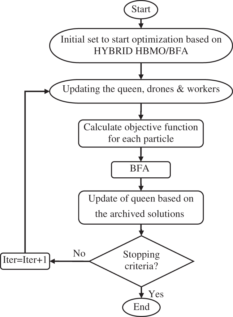
Figure 1: The flowchart of suggested hybrid HBMO/BFA technique

4  Numeric Results

In this section, the robust security-constrained UC programming problem in the presence of wind farm and ESS obtained in the previous section is implemented on two test systems: a six-bus test grid and a 24-bus IEEE transfer grid; the capabilities of the proposed model are also examined.

4.1 Six-Bus Test Grid

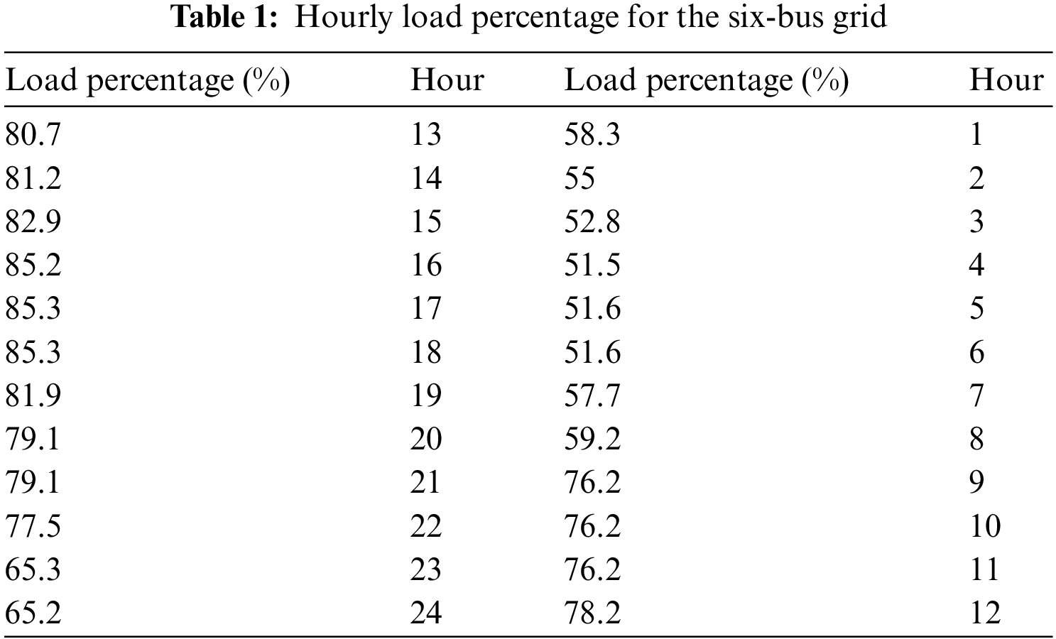
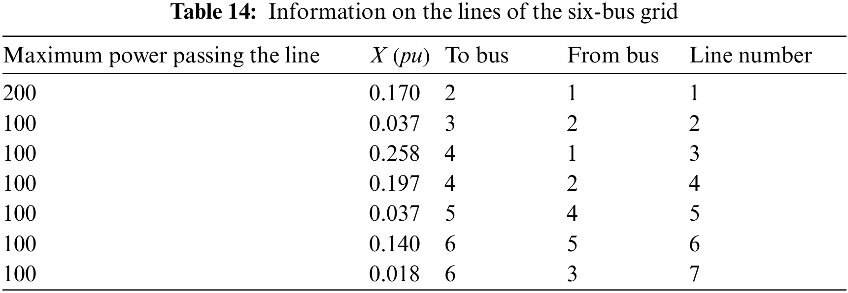
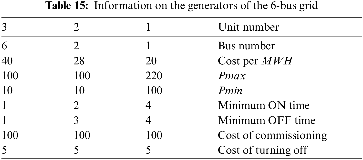
The security-constrained UC programming by using optimization in the presence of wind farm and ESS for 24 h is implemented on a six-bus grid (specifications in Appendix A and single-line diagram in Fig. 2. This grid has three generators, seven lines and six buses, and serves as a small grid for better understanding the concepts. Fig. 2 depicts the single-line diagram of this grid. Loads in buses 3, 4 and 5 make up respectively 20%, 40% and 40% of the total load of the grid that is 216 MW. The hourly load is obtained by multiplying the total load by load percentage (Table 1).

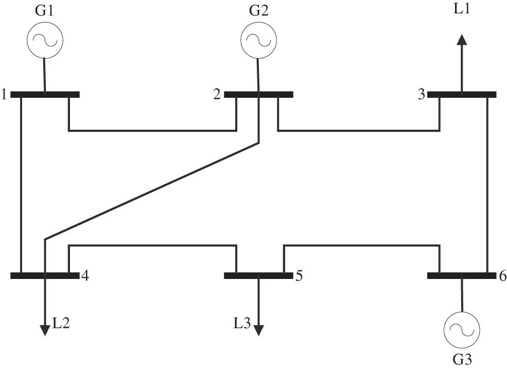
Figure 2: Single-line diagram of six bus grid

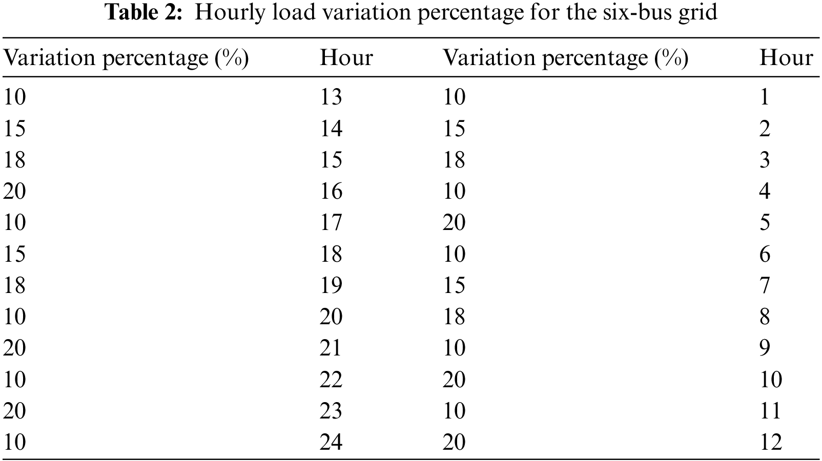
Due to the load uncertainty, the percentage of variations in Table 2 is assumed for the load of this test grid.

A 20 MW wind farm is added to the examined grid on bus 4. The hourly wind-generated power is calculated by multiplying 20 MW by the wind percentage in Table 3. However, since the WT output has variations, the same load variation percentage is assumed for the hourly deterministic wind power variations.

An ESS is also added to bus 5 (Table 4).

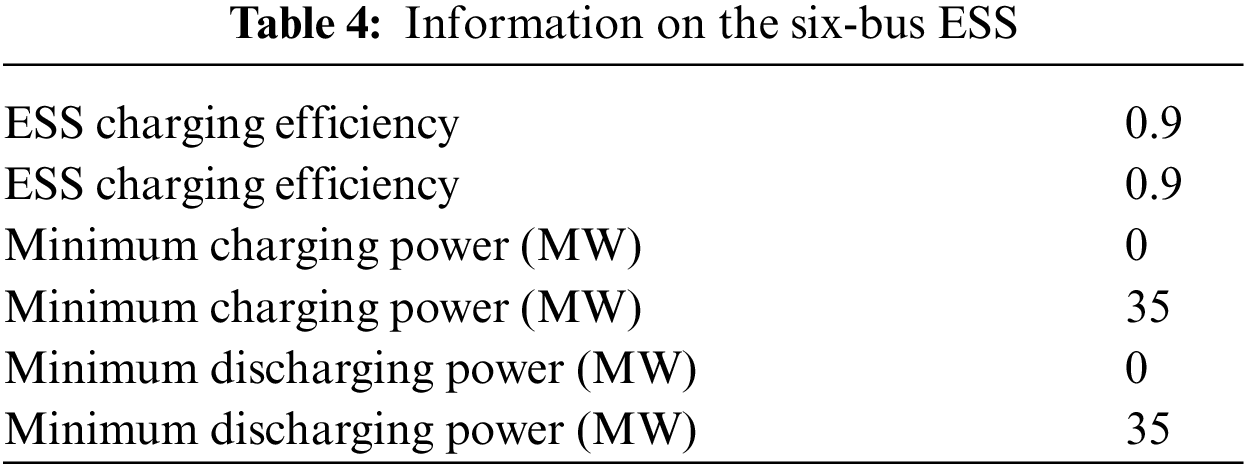
The maximum and minimum hourly capacity of the ESS is 90 and 0 MW, respectively. The cost per MWh of ESS charging is $0.5 and the cost per MWh of ESS discharging is $0.1.

4.2 Results of the SCUC Model without the Wind Farm and ESS

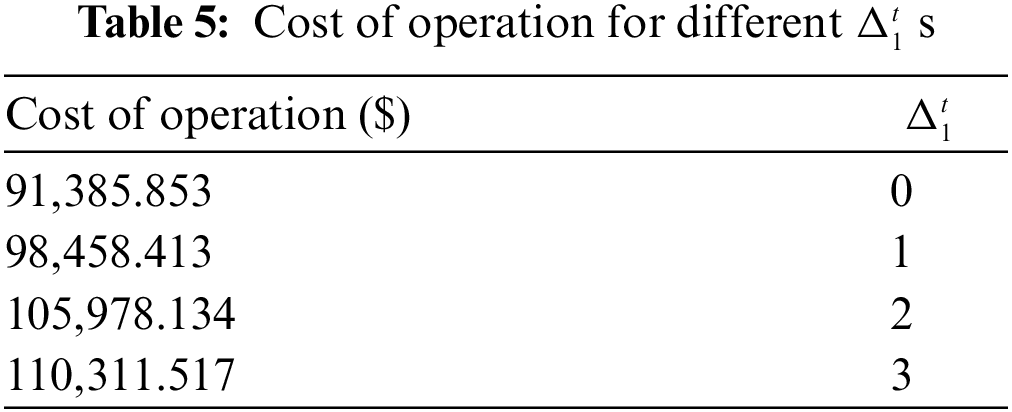
The security-constrained UC programming problem is first solved without the wind farm and ESS by using optimization for the load uncertainty budget of Δ1t=0 (deterministic case) and Δ1t=1, Δ1t=2 and Δ1t=3. Fig. 3 displays the load variation interval, deterministic load and load for different values of the uncertainty budget parameter. Table 5 lists the cost of operation for different values of the uncertainty budget parameter. Based on Fig. 3, by increasing Δ1t, more deviation is made from the predicted load value; therefore, solving the SCUC problem will yield more conservative results and the system will be protected against further variations in load uncertainty. In Δ1t=3, the SCUC problem is programmed for the worst-case load determinism conditions (maximum load that may occur in real time).

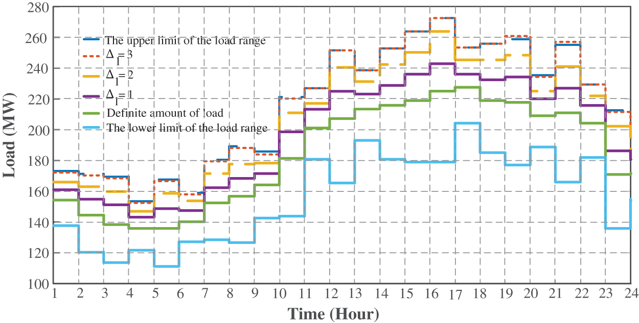
Figure 3: Load uncertainty variation interval and its value per different Δ1ts

By raising Δ1t, the system confidence is promoted, but the costs of operation also rise due to the need for more units to cover a wider range of uncertainties (Table 5).

4.3 Results of the SCUC Model in the Presence of the Wind Farm and without ESS

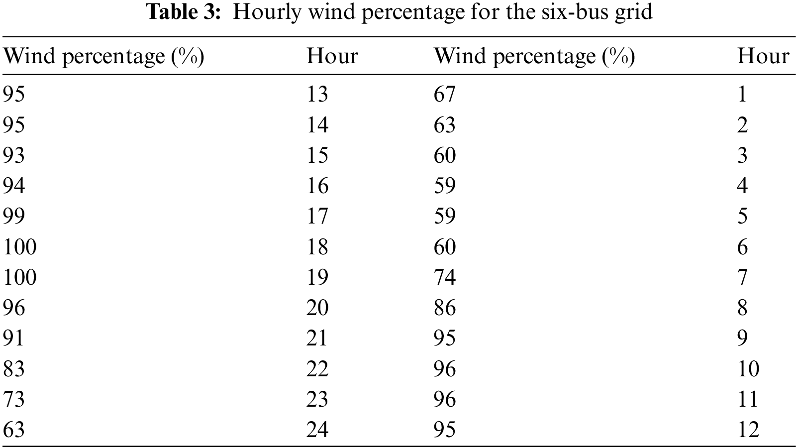
In this case, we assume the wind farm exists in the grid without the ESS. Based on the wind farm-generated power uncertainty, the SCUC problem is solved for the worst-case scenario of load uncertainty (Δ1t=3) and wind uncertainty parameter of Δ2t=0 (deterministic), Δ2t=0.5 and Δ2t=1. Fig. 4 displays the variation interval, deterministic circuit and wind farm-generated power for different values of the wind uncertainty budget parameter. Table 6 lists the cost of operation for different values of the wind uncertainty budget parameter. By increasing the wind uncertainty budget from 0 to 0.5 as the result of a decrease in wind farm power generation, the total cost is increased from 98,501.532 to 99,238.942. By setting the wind uncertainty budget to 1, the wind farm power generation is minimized. Thus, by increasing Δ2t, the cost of operation also rises and more accurate programming is achieved; therefore, the use of the model reduces the grid's confidence when incorporating wind farms. To promote grid confidence and power quality for users, we will utilize an ESS in addition to the model when using the wind farm.

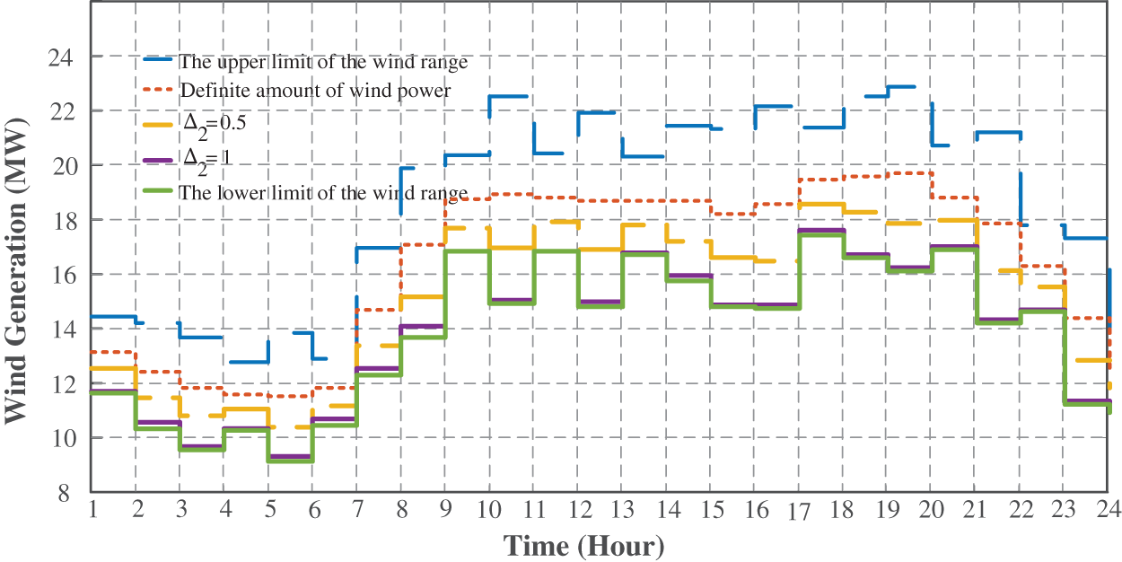
Figure 4: Wind-generated power uncertainty variation interval and its value for different Δ2ts

4.4 Results of the SCUC Model in the Presence of the Wind Farm and ESS

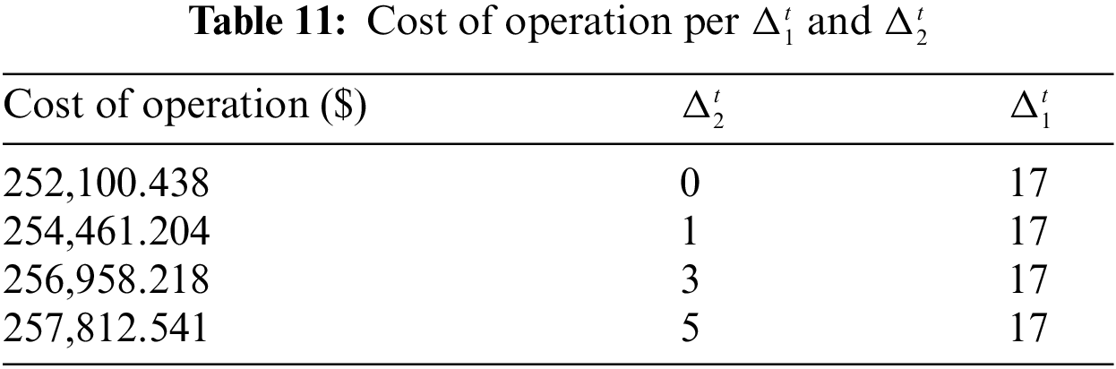
The SCUC problem is solved in the presence of a wind farm and ESS with load and wind farm-generated power uncertainties by using the model for the worst-case uncertainty scenario (Δ1t=3 and Δ2t=1). The load and wind farm-generated power are based on Figs. 3 and 4. The cost of operation of the grid without the ESS is 100,105.718, but it is reduced to $99,103.917 in the presence of the ESS.

Based on Fig. 5, this cost reduction when using the ESS is due to charging the ESS by cheap power stations during non-peak hours and discharging it during peak hours. Thus, the use of the ESS reduces the cost of operation, promotes system confidence and improves the power quality, which are important issues.

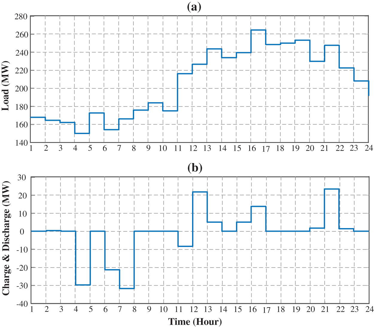
Figure 5: ESS charge/discharge power and grid load (Δ1t=3 and Δ2t=1)

4.5 The 24-Bus Test Grid

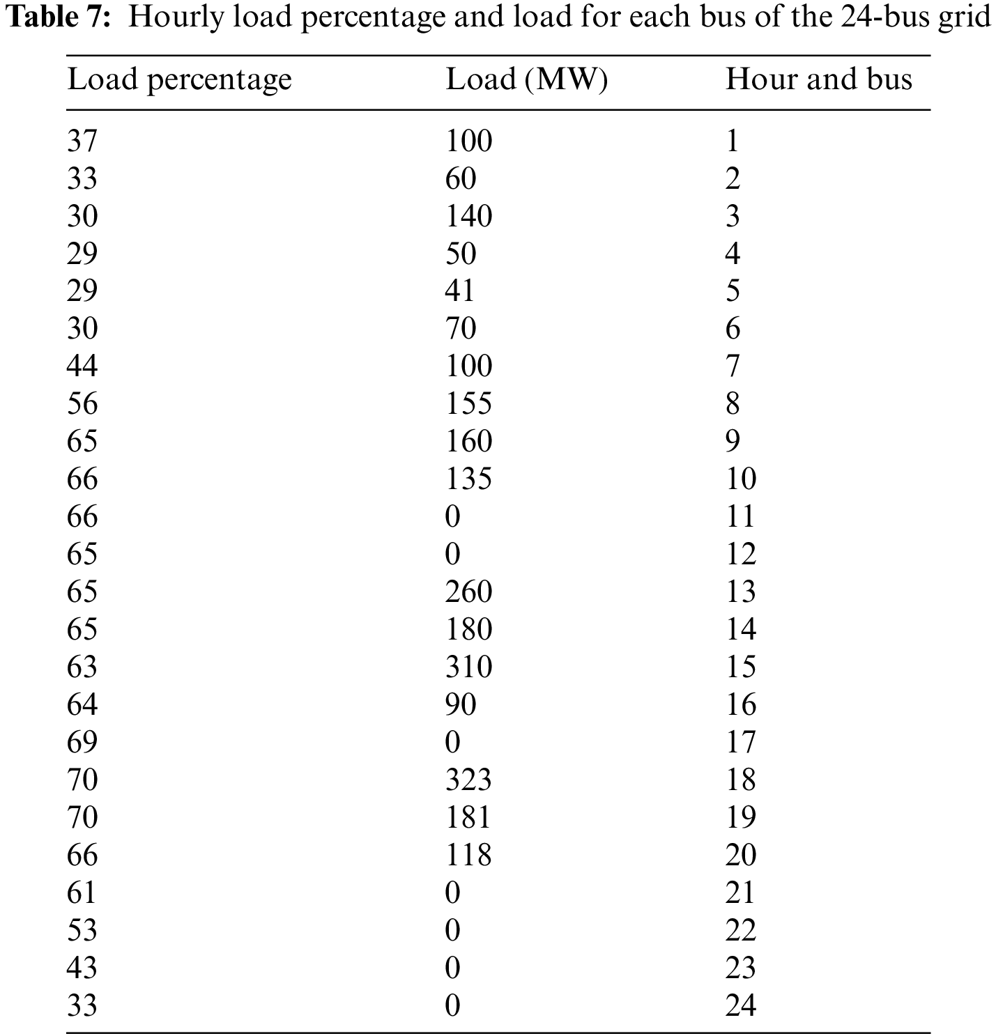
Herein, the model proposed in Section 2 is applied to a larger grid. To this end, a 24-bus IEEE grid is selected (costs of units and single-line diagram in [31] and cost of units’ commissioning in [32]). In the deterministic state, the hourly load for each bus is attained by multiplying the load by the hourly load percentage (the load and load percentage given in Table 7). Based on the uncertainty assumed for the load, its variation percentage for this grid is similar to the six-bus grid.

4.6 Results of the SCUC Model without the Wind Farm and ESS

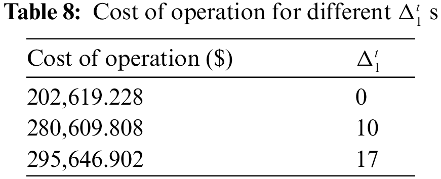
Based on Fig. 6, by increasing Δ1t, a larger part of the load uncertainty interval is covered, so that at Δ1t=17, the worst-case scenario of load uncertainty is assumed. As a result, the grid is promoted against load uncertainty and system confidence. However, this promotion in system confidence is associated with a rise in costs (Table 8). In other words, the problem's optimality is diminished. One can select Δ1t such that the intended gird confidence and optimality can be attained.

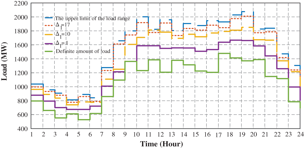
Figure 6: Load uncertainty variation interval and its value per different Δ1ts

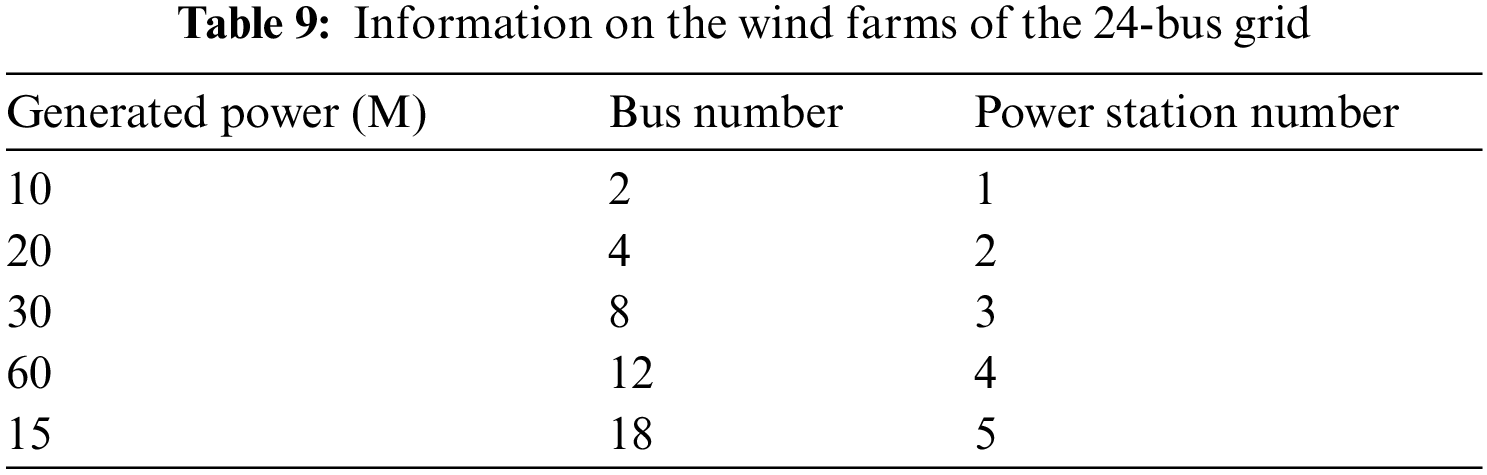
4.7 Results of the SCUC Model in the Presence of Wind Farm and without ESS

In this case, we assume that only a wind farm is added to the grid in the worst-case load uncertainty scenario (Δ1t=17). Table 9 lists the information on the wind farms in the standard IEEE 24-bus grid. As the scheduling interval is 24 h, a coefficient known as wind percentage is presented in Table 10. Each power station's hourly generated electric power is calculated via multiplying the power station's nominal power by the wind percentage. As uncertainty is assumed for the electric power generated by the wind farms, the generated electric power variation percentage is assumed to be the same as the load variations.

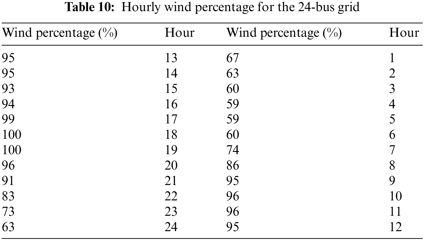
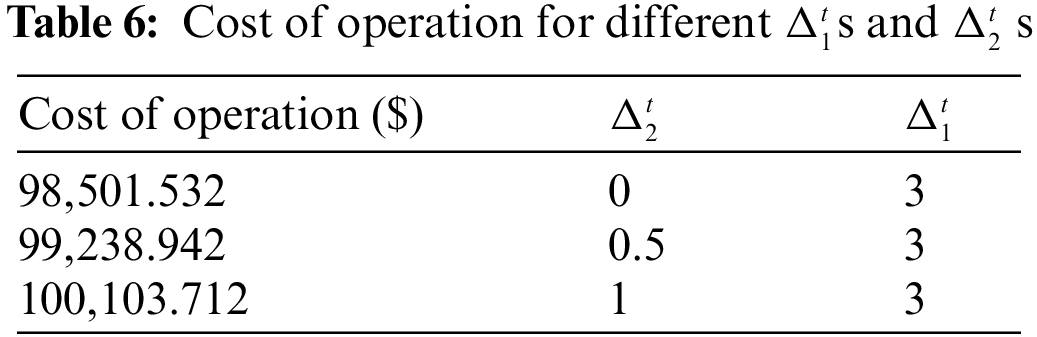
Based on Fig. 7, by increasing Δ2t, the value obtained for the wind farm-generated power in the security-constrained UC programming problem approaches the lower limit of the wind farm-generated power prediction interval. At Δ2t=5 (maximum Δ2t that is equal to the number of wind farms, the output of which has uncertainty), the worst case of wind farm-generated power uncertainty is assumed. Consequently, the grid against the wind farm-generated power uncertainty and the system confidence has increased (in other words, the probability of power supply deficit through wind farms in real time is much reduced). Nevertheless, this promotion in system confidence is associated with a rise in costs (Table 11). Increasing Δ2t is associated with a decline in wind farm-generated power; as a result, power is supplied from more expensive thermal power stations. In other words, the problem's optimality is diminished. One can select Δ2t, such that the intended gird confidence and optimality can be attained.

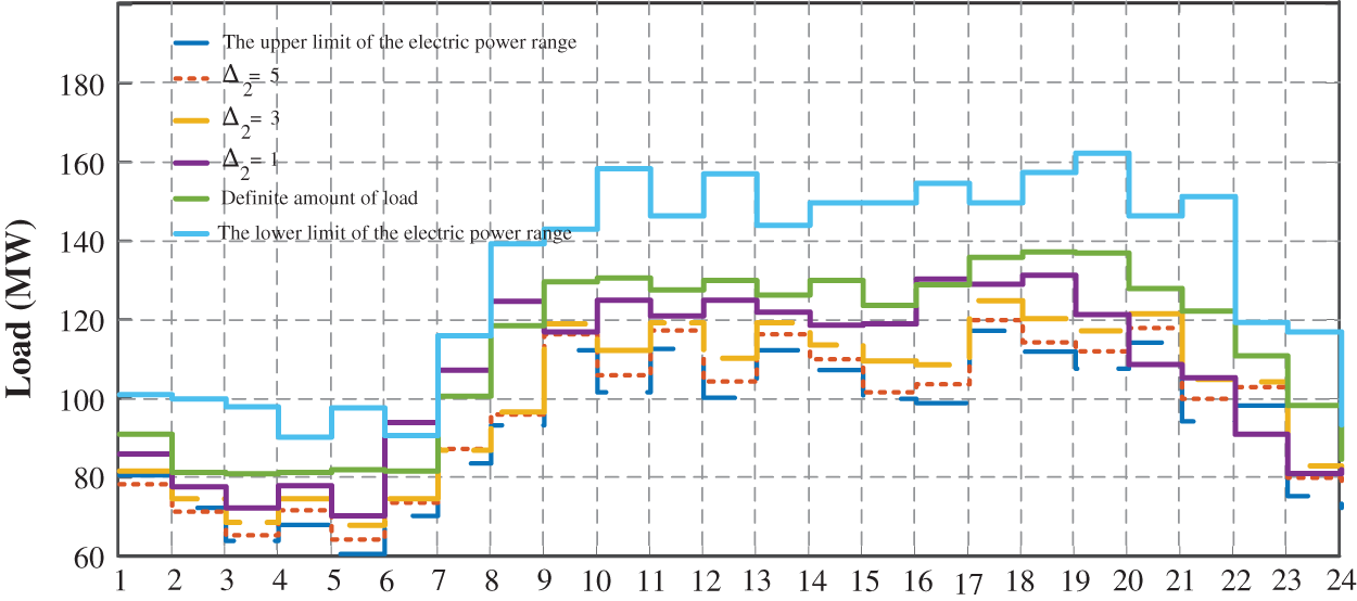
Figure 7: Wind-generated power uncertainty variation interval and its value for different Δ2ts

4.8 Results of the SCUC Model in the Presence of the Wind Farm and ESS

To observe the effect of ESS, this equipment is assumed for the power system in this grid (Table 12). The maximum and minimum hourly capacities of the ESS are 100 and 0 MW, respectively. The cost per MWh of ESS charging is $0.5 and the cost per MWh of ESS discharging is $0.1. The initial and final energies of the ESS are assumed to be 0. The ESS charge/discharge power and grid load is presented in Fig. 8.

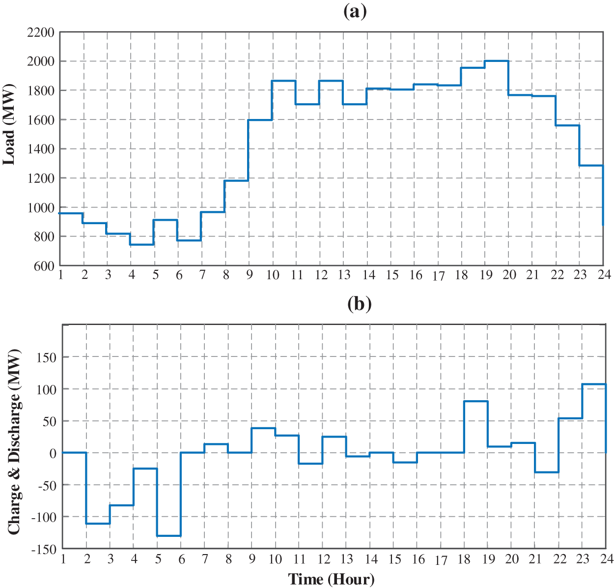
Figure 8: ESS charge/discharge power and grid load (Δ1t=3 and Δ2t=1)

Table 13 presents the hourly charge/discharge level of the ESS for the worst case of load uncertainty and wind farm-generated power. Negative values in this table indicate charging (consumption), and positive values denote discharging (generation) of the ESS.

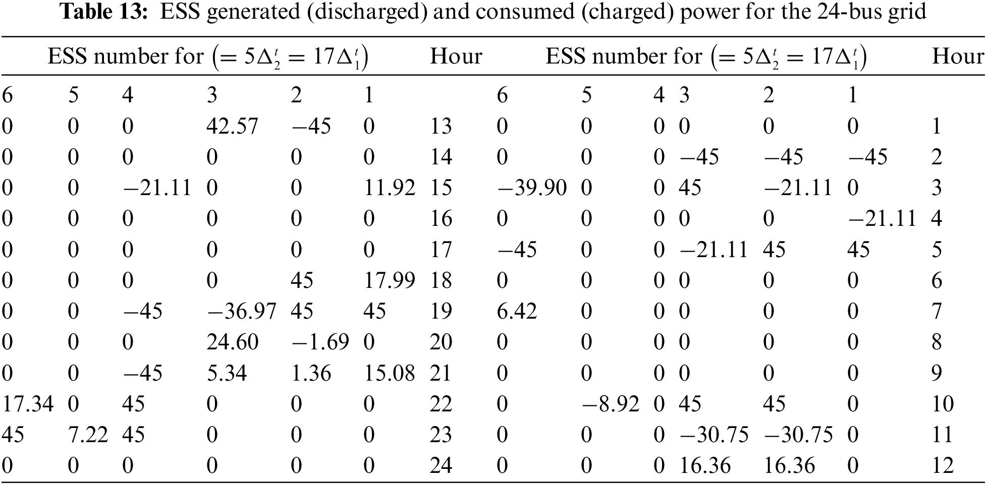
The use of the ESS has reduced costs from $257,829.495 to $250,748.726 for the worst case of load and wind farm-generated power uncertainty. This cost reduction is due to ESS charging in non-peak and discharging in peak hours. ESS also improves system confidence and power quality, which are important issues.

To show the efficiency of proposed model, we applied classic BFA and HBMO for solving this problem. In this comparison, the proposed hybrid model is compared with two basic models. Accordingly, the HBMO could calculate the cost from $264,674.22 and reduce it by considering the ESS to $257,662.14. this value is $264,975.41 and reduce it to $258,674.63 by considering ESS. Consequently, this comparison shows the superiority of proposed hybrid algorithm in comparison with basic models.

5  Conclusion

RES such as WT and solar cells have attracted the attention of power system operators and users alike due to their lack of environmental pollution, independence of fossil fuels, and low marginal costs. With the introduction of RES, challenges have faced the solution of the UC problem as a traditional power system optimization problem aiming to minimize total costs by optimally determining units’ inputs and outputs, and specifying the optimal generation of each unit. The output power of RES such as WT and solar cells depends on natural factors such as wind speed and solar irradiation that are riddled with uncertainty. As a result, the UC problem in the presence of RES faces uncertainties. The grid consumed load is not always equal to and is randomly different from the predicted values, which also contributes to uncertainty in solving the aforementioned problem. To model load uncertainty as well as wind and solar power station uncertainty, stochastic solving methods and probabilistic methods can be adopted by allocating proper probability density functions (PDF) to the uncertainty factors. The present study adopted a novel method to perform security-constrained UC programming in the presence of a wind farm and ESS with load and wind farm-generated power uncertainty. The proposed model minimized the grid operating cost for the worst case of load uncertainty. For this purpose, new approach is presented in this paper based on an uncertain optimization model that is the stochastic with security-constrains consisting of undispatchable power resources and storage units. By using a hybrid HBMO and bacterial foraging algorithm, the optimal unit commissioning/decommissioning and the optimal generation of each unit were determined. The proposed approach may trap in local minima while, combination of this algorithm could solve this problem and get suitable outcome in comparison with other models. The simulation results revealed that the ESS equipment in the power system improved power quality and confidence and reduced the peak and costs.

Funding Statement: The authors received no specific funding for this study.

Conflicts of Interest: The authors declare that they have no conflicts of interest to report regarding the present study.

References

 1.  Cao, W., Pan, X., Sobhani, B. (2021). Integrated demand response based on household and photovoltaic load and oscillations effects. International Journal of Hydrogen Energy, 46(79), 39523–39535. DOI 10.1016/j.ijhydene.2021.08.212. [Google Scholar] [CrossRef]

 2.  Akbarimajd, A., Sobhani, B. (2014). Optimal lead-lag controller for distributed generation unit in island mode using simulated annealing. Computational Intelligence in Electrical Engineering, 5(2), 17–28. [Google Scholar]

 3.  Shayanfar, H. A., Abedinia, O., Amjady, N. (2015). Solving unit commitment problem based on New stochastic search algorithm. Proceedings on the International Conference on Artificial Intelligence (ICAI), pp. 105. Los Vegas, USA, The Steering Committee of the World Congress in Computer Science, Computer Engineering and Applied Computing (WorldComp). [Google Scholar]

 4.  Shayeghi, H., Firoozjaee, H. G., Ghasemi, A., Abedinia, O., Bazyar, R. (2012). Optimal thermal generating unit commitment with wind power impact: A PSO-IIW procedure. International Journal on Technical and Physical Problems of Engineering, 4(11), 90–97. [Google Scholar]

 5.  Kwon, K. B., Kim, D. (2020). Enhanced method for considering energy storage systems as ancillary service resources in stochastic unit commitment. Energy, 213, 118675. DOI 10.1016/j.energy.2020.118675. [Google Scholar] [CrossRef]

 6.  Howlader, H. O. R., Adewuyi, O. B., Hong, Y. Y., Mandal, P., Mohamed Hemeida, A. et al. (2020). Energy storage system analysis review for optimal unit commitment. Energies, 13(1), 158. DOI 10.3390/en13010158. [Google Scholar] [CrossRef]

 7.  Xiong, P., Jirutitijaroen, P., Singh, C. (2016). A distributionally robust optimization model for unit commitment considering uncertain wind power generation. IEEE Transactions on Power Systems, 32(1), 39–49. DOI 10.1109/TPWRS.2016.2544795. [Google Scholar] [CrossRef]

 8.  Jiang, R., Wang, J., Guan, Y. (2011). Robust unit commitment with wind power and pumped storage hydro. IEEE Transactions on Power Systems, 27(2), 800–810. DOI 10.1109/TPWRS.2011.2169817. [Google Scholar] [CrossRef]

 9.  Li, J., Zhou, S., Xu, Y., Zhu, M., Ye, L. (2021). A multi-band uncertainty set robust method for unit commitment with wind power generation. International Journal of Electrical Power & Energy Systems, 131, 107125. DOI 10.1016/j.ijepes.2021.107125. [Google Scholar] [CrossRef]

10. AlHajri, I., Ahmadian, A., Elkamel, A. (2021). Stochastic day-ahead unit commitment scheduling of integrated electricity and gas networks with hydrogen energy storage (HESplug-in electric vehicles (PEVs) and renewable energies. Sustainable Cities and Society, 67, 102736. DOI 10.1016/j.scs.2021.102736. [Google Scholar] [CrossRef]

11. Wang, S., Zheng, N., Bothwell, C. D., Xu, Q., Kasina, S. et al. (2021). Crediting variable renewable energy and energy storage in capacity markets: Effects of unit commitment and storage operation. IEEE Transactions on Power Systems, 37(1), 617–628. DOI 10.1109/TPWRS.2021.3094408. [Google Scholar] [CrossRef]

12. Xu, J., Ma, Y., Li, K., Li, Z. (2021). Unit commitment of power system with large-scale wind power considering multi time scale flexibility contribution of demand response. Energy Reports, 7, 342–352. DOI 10.1016/j.egyr.2021.10.025. [Google Scholar] [CrossRef]

13. Salimi, A. A., Karimi, A., Noorizadeh, Y. (2019). Simultaneous operation of wind and pumped storage hydropower plants in a linearized security-constrained unit commitment model for high wind energy penetration. Journal of Energy Storage, 22, 318–330. DOI 10.1016/j.est.2019.02.026. [Google Scholar] [CrossRef]

14. Pozo, D., Contreras, J., Sauma, E. E. (2014). Unit commitment with ideal and generic energy storage units. IEEE Transactions on Power Systems, 29(6), 2974–2984. DOI 10.1109/TPWRS.2014.2313513. [Google Scholar] [CrossRef]

15. Rezaee Jordehi, A. (2021). An improved particle swarm optimisation for unit commitment in microgrids with battery energy storage systems considering battery degradation and uncertainties. International Journal of Energy Research, 45(1), 727–744. DOI 10.1002/er.5867. [Google Scholar] [CrossRef]

16. Zhang, C., Dong, Z., Yang, L. (2021). A feasibility pump based solution algorithm for two-stage robust optimization with integer recourses of energy storage systems. IEEE Transactions on Sustainable Energy, 12(3), 1834–1837. DOI 10.1109/TSTE.2021.3053143. [Google Scholar] [CrossRef]

17. Zhu, T., Wang, Z., Zhao, C., Xu, S. (2020). Two-stage stochastic dynamic unit commitment and Its analytical solution with large scale wind power integration. 2020 IEEE 4th Conference on Energy Internet and Energy System Integration (EI2), pp. 2016–2022. Wuhan, China, IEEE. [Google Scholar]

18. Aghaei, J., Rahimi Rezaei, A., Karimi, M. (2018). Coordination of wind power plants and energy storage devices in security-constrained unit commitment problem using robust optimization. Journal of Modeling in Engineering, 16(53), 207–220. DOI 10.22075/JME.2017.5881. [Google Scholar] [CrossRef]

19. Alqunun, K., Guesmi, T., Albaker, A. F., Alturki, M. T. (2020). Stochastic unit commitment problem, incorporating wind power and an energy storage system. Sustainability, 12(23), 10100. DOI 10.3390/su122310100. [Google Scholar] [CrossRef]

20. Kiran, B. D. H., Kumari, M. S. (2016). Demand response and pumped hydro storage scheduling for balancing wind power uncertainties: A probabilistic unit commitment approach. International Journal of Electrical Power & Energy Systems, 81, 114–122. DOI 10.1016/j.ijepes.2016.02.009. [Google Scholar] [CrossRef]

21. Ebrahimi, H., Abapour, M., Mohammadi-Ivatloo, B., Golshannavaz, S., Yazdaninejadi, A. (2021). Decentralized approach for security enhancement of wind-integrated energy systems coordinated with energy storages. International Journal of Energy Research, 46(4), 5006–5027. DOI 10.1002/er.7494. [Google Scholar] [CrossRef]

22. Malekshah, S., Banihashemi, F., Daryabad, H., Yavarishad, N., Cuzner, R. (2022). A zonal optimization solution to reliability security constraint unit commitment with wind uncertainty. Computers & Electrical Engineering, 99, 107750. DOI 10.1016/j.compeleceng.2022.107750. [Google Scholar] [CrossRef]

23. Zou, Y., Zhao, J., Ding, D., Miao, F., Sobhani, B. (2021). Solving dynamic economic and emission dispatch in power system integrated electric vehicle and wind turbine using multi-objective virus colony search algorithm. Sustainable Cities and Society, 67, 102722. DOI 10.1016/j.scs.2021.102722. [Google Scholar] [CrossRef]

24. Malekshah, S., Ansari, J. (2021). A novel decentralized method based on the system engineering concept for reliability-security constraint unit commitment in restructured power environment. International Journal of Energy Research, 45(1), 703–726. DOI 10.1002/er.5802. [Google Scholar] [CrossRef]

25. Malekshah, S., Malekshah, Y., Malekshah, A. (2021). A novel two-stage optimization method for the reliability based security constraints unit commitment in presence of wind units. Cleaner Engineering and Technology, 4, 100237. DOI 10.1016/j.clet.2021.100237. [Google Scholar] [CrossRef]

26. Çiçek, A., Erdinç, O. (2021). Risk-averse optimal bidding strategy considering bi-level approach for a renewable energy portfolio manager including EV parking lots for imbalance mitigation. Sustainable Energy, Grids and Networks, 28, 100539. DOI 10.1016/j.segan.2021.100539. [Google Scholar] [CrossRef]

27. Ebrahimi, H., Yazdaninejadi, A., Golshannavaz, S. (2022). Demand response programs in power systems with energy storage system-coordinated wind energy sources: A security-constrained problem. Journal of Cleaner Production, 335, 130342. DOI 10.1016/j.jclepro.2021.130342. [Google Scholar] [CrossRef]

28. Abedinia, O., Naderi, M. S., Ghasemi, A. (2011). Robust LFC in deregulated environment: Fuzzy PID using HBMO. 2011 10th International Conference on Environment and Electrical Engineering, pp. 1–4. Rome, Italy, IEEE. DOI 10.1109/EEEIC.2011.5874843. [Google Scholar] [CrossRef]

29. Taheri, S. I., Salles, M. B., Nassif, A. B. (2021). Distributed energy resource placement considering hosting capacity by combining teaching–learning-based and honey-bee-mating optimisation algorithms. Applied Soft Computing, 113, 107953. DOI 10.1016/j.asoc.2021.107953. [Google Scholar] [CrossRef]

30. Zhang, X., Wang, Z., Lu, Z. (2022). Multi-objective load dispatch for microgrid with electric vehicles using modified gravitational search and particle swarm optimization algorithm. Applied Energy, 306, 118018. DOI 10.1016/j.apenergy.2021.118018. [Google Scholar] [CrossRef]

31. Hedman, K. W., Ferris, M. C., O'Neill, R. P., Fisher, E. B., Oren, S. S. (2010). Co-optimization of generation unit commitment and transmission switching with N-1 reliability. IEEE Transactions on Power Systems, 25(2), 1052–1063. DOI 10.1109/TPWRS.2009.2037232. [Google Scholar] [CrossRef]

32. Hedman, K. W., O'Neill, R. P., Fisher, E. B., Oren, S. S. (2009). Optimal transmission switching with contingency analysis. IEEE Transactions on Power Systems, 24(3), 1577–1586. DOI 10.1109/TPWRS.2009.2020530. [Google Scholar] [CrossRef]

Appendix A

The specifications of lines and generators of the six-bus grid are given in Tables 14 and 15.

This work is licensed under a Creative Commons Attribution 4.0 International License, which permits unrestricted use, distribution, and reproduction in any medium, provided the original work is properly cited.