DOI: 10.32604/fdmp.2021.013497
ARTICLE
Numerical Simulations of Hydromagnetic Mixed Convection Flow of Nanofluids inside a Triangular Cavity on the Basis of a Two-Component Nonhomogeneous Mathematical Model
1Department of Mathematics, College of Science, Sultan Qaboos University, Muscat, Oman
2Department of Mathematics, Jagannath University, Dhaka, Bangladesh
*Corresponding Author: M. M. Rahman. Email: mansurdu@yahoo.com; mansur@squ.edu.om
Received: 08 August 2020; Accepted: 24 December 2020
Abstract: Nanofluids have enjoyed a widespread use in many technological applications due to their peculiar properties. Numerical simulations are presented about the unsteady behavior of mixed convection of Fe3O4-water, Fe3O4- kerosene, Fe3O4-ethylene glycol, and Fe3O4-engine oil nanofluids inside a lid-driven triangular cavity. In particular, a two-component non-homogeneous nanofluid model is used. The bottom wall of the enclosure is insulated, whereas the inclined wall is kept a constant (cold) temperature and various temperature laws are assumed for the vertical wall, namely:  (Case 1),
  (Case 2), and
 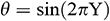 (Case 3). A tilted magnetic field of uniform strength is also present in the fluid domain. From a numerical point of view, the problem is addressed using the Galerkin weighted residual finite element method. The role played by different parameters is assessed, discussed critically and interpreted from a physical standpoint. We find that a higher aspect ratio can produce an increase in the average Nusselt number. Moreover, the Fe3O4-EO and Fe3O4-H2O nanofluids provide the highest and smallest rate of heat transfer, respectively, for all the considered (three variants of) thermal boundary conditions.
Keywords: Nanofluid; mixed convection; lid-driven; triangular cavity; finite element method
Nomenclature
 : : | dimensional amplitude of the wave (m) |
 : : | aspect ratio |
 : : | magnetic field strength (kgs-2A-1) |
 : : | specific heat at constant pressure (Jkg-1K-1) |
 : : | nanoparticle volume fraction |
 : : | Brownian diffusion coefficient (m2s-1) |
 : : | thermophoretic diffusion coefficient (m2s-1) |
 : : | gravitational acceleration (ms-1) |
 : : | height of the cavity (m) |
 : : | Hartmann number |
 : : | thermal conductivity (Wm-1K-1) |
 : : | wave number |
 : : | length of the cavity (m) |
 : : | Lewis number |
 : : | Brownian motion parameter |
 : : | buoyancy ratio parameter |
 : : | thermophoresis parameter |
 : : | Nusselt number |
 : : | dimensional pressure (Pa) |
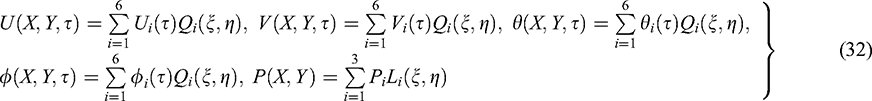
 : : | dimensionless pressure |
 : : | Prandtl number |
| Ri : | Richardson number |
 : : | temperature (K) |
 : : | dimensional velocity components (ms-1) |
 : : | dimensionless velocity components |
 : : | dimensional coordinates (m) |
 : : | dimensionless coordinates |
Greek symbols
 : : | thermal diffusivity (m2s-1) |
 : : | coefficient of thermal expansion (K-1) |
 : : | magnetic inclination angle (degree) |
 : : | electric conductivity (Wm-1K-1) |
 : : | dimensionless temperature |
 : : | normalized nanoparticle volume fraction |
 : : | stream function (m2s-1) |
 : : | dynamic viscosity (Pas) |
 : : | density (kgm-3) |
 : : | heat capacity (JK-1m-3) |
Subscripts
| ave: | average |
| c: | condition at cold wall |
| f: | base fluid |
| h: | condition at heated wall |
| p: | solid nanoparticle |
The overheating limits the lifespan of the usage of electronic pieces of equipment (for example, computer processor) while operating. It is a big challenge for the industries which produce such sophisticated types of equipment. In a recent study, Bayomy et al. [1] reported that the efficiency rate of electronic devices decreases exponentially due to heat generation within them. The traditional fluids (water, mineral oils, and ethylene glycol) most of the time used for industrial cooling applications limit their use as efficient heat transfer agent. For the growing need in modern technology (chemical production, power station, a computer processor, and micro-electronics), researchers developed nanofluid [2], which efficiently transmit heat. Nanofluid exhibits higher thermal conductivity hence enhanced heat transfer compared to the conventional fluids [3–13] even in the presence of a small amount (1%–5% volume fraction) of nanoparticles.
The heat transfer enhancement inside cavities has become a paramount issue in the industrial and energy sectors. Many researchers studied nanofluids experimentally, analytically as well as numerically for heat enhancement in cavities. In this respect, Khanafer et al. [14] studied the heat transfer enhancement in a differentially heated square cavity. They found that the suspended nanoparticles considerably increase the heat transfer rate. Oztop et al. [15] conducted a numerical study considering the natural convection flow inside the partially heated rectangular enclosure filled with nanofluids. They found that the mean Nusselt number increases with the increase of the nanoparticles volume fraction. They further reported that the low aspect ratio of the geometry significantly enhances the heat transfer rate in nanofluids compared to the corresponding heat transfer for a high aspect ratio.
Magnetohydrodynamics (MHD) convective flow has widespread applications in science and engineering such as extraction of geothermal energy, oil recovery from the petroleum reservoirs, thermal insulation, cooling of nuclear reactors, crystal growth, and plasma confinement [16–18]. In light of the various applications of MHD and nanofluids, Al Kalbani et al. [19,20] investigated the buoyancy induced heat transfer flow inside a tilted square cavity filled with nanofluids in the presence of an oriented magnetic field. Their results confirm that the nanoparticle volume fraction, shape, and size significantly intensified the heat transfer rate inside a crater. The applied magnetic field and its direction also played a vital role in heat enhancement. Al Balushi et al. [21,22] further investigated the free convection heat transfer flow of nanofluids inside square cavities utilizing nanofluids under the action of an applied inclined magnetic field to the flow domain. They used a nonhomogeneous dynamic model for nanofluid modeling. They found that heat enhancement in nanofluids depends on the nanoparticle loading, magnetic field’s direction and strength, and the location of the heater that supplies heat to the flow field.
The thermal discharge in lid-driven enclosures has direct applications in many engineering fields such as in rheology for lubrication mechanisms, cooling of electronic devices, constructing buildings roofs and attics, processing food, and cooling nuclear reactors (see [23]). Flack et al. [24,25] studied experimentally as well as numerically the convective heat transfer in triangular enclosures. Later on, many researchers conducted research and reported results on triangular-cavities [26–31]. All of these studies involved heat transfer in regular fluids. Due to the growing need for nanofluid research in triangular cavities, Ghasemi et al. [32] studied numerically; the steady natural convection flow of CuO-water nanofluid inside a fixed-walls right triangular enclosure. They reported that the Brownian motion of nanoparticles takes part in enhancing the thermal performance of nanofluids in a cavity. Ghasemi et al. [33] further studied steady mixed convection in a lid-driven triangular enclosure filled with Al2O3-water nanofluid. They confirmed that enhancement in heat transfer within the cavity is due to the addition of nanoparticles, and it depends on the direction of the sliding wall motion. Rahman et al. [34] conducted a numerical study on hydromagnetic free convection flow of nanofluids inside an isosceles-triangular cavity. In their simulation, they used the two-component nonhomogeneous mathematical model and different thermal conditions. The results show that the variable thermal boundary conditions have significant effects on the flow and thermal fields. Rahman [35] studied the hydromagnetic natural convection flow and heat transfer within an equilateral triangular enclosure. In his work, he used water-based as well as kerosene-based ferrofluids in the presence of a sloping magnetic field. The results indicate that increased magnetic field strength diminishes the heat transfer rate, whereas it enhances with the increment of the magnetic field inclination angle. Rahman [36] further studied steady heat transfer in Fe3O4-water nanofluid inside a triangular cavity with fixed walls under a sloping magnetic field. They conclude that a higher degree of heat transfer is accomplished by reducing the dimension of nanoparticles and increasing the strength of the buoyancy force. Azam et al. [37–41] published a series of papers on unsteady heat and mass transfer flow of nanofluids in different geometries with the various flow and thermal conditions proposed by the Buongiorno mathematical model. In a recent study, Uddin et al. [42] explored heat transportation in copper oxide-water nanofluid inside different triangular cavities. Their results show that heat enhancement in nanofluids strongly depends on the shape of the triangular shape cavity and the applied buoyancy force.
Despite significant research studies on various cavities reported in the literature, there is a substantial lack of information regarding the problem of time-dependent hydromagnetic fluid flow and heat transfer enhancement in the lid-driven right triangular-cavity filled with nanofluids. Therefore, the present paper aims to investigate numerically unsteady mixed convection flow and heat transfer in a lid-driven right-triangular cavity filled with different types of nanofluids in the presence of an oriented magnetic field varying aspect ratio of the enclosure taking into account the Buongiorno mathematical model. We used the Galerkin weighted residual-based finite element method for numerical simulation. Finally, we depicted the mean rate of heat transfer in terms of Nusselt number in varying different model parameters. The organization of the remainder of the paper is as follows: In Section 2, we formulate the problem physically as well as mathematically. Section 3 explains the method of solution in detail. The numerical outcomes we discuss from physical and engineering viewpoints in Section 4. In the end, in Section 5, we conclude our study.
We consider an unsteady, laminar, incompressible two-dimensional mixed convection flow inside a right-angle triangular cavity that is filled with Fe3O4-water nanofluid as shown in Fig. 1, where  and
and  are the Cartesian coordinates. Here,
  is the bottom wall length, and
  is the height of the vertical wall. We assumed that the vertical wall temperature is
  while the inclined wall (hypotenuse) is
  (where
  ). The bottom-wall is insulated; thus, no heat can escape along the transverse direction of it. Initially, we considered that nanofluid concentration is
  , but for
  , it is assumed as
  in the entire domain so that
  . The vertical wall is allowed to move with constant speed
  in its plane while the remaining walls have no speed. Here the gravity acts in the vertical direction, along the
  -axis. We included the thermophoresis and Brownian diffusion effects in the mathematical model in the absence of any chemical reaction and thermal radiation. The base fluid and the nanoparticles are in thermal equilibrium, and hence no slip occurs between them. Surfactant or surface charge technology disperses the nanoparticles within the nanofluid. The Boussinesq approximation tackled the density variation in the buoyancy force.
Figure 1: Schematic view of the physical model with boundary conditions
The cavity is permeated by a uniform magnetic field  of constant magnitude
  , where
  and
and  are the unit vectors along the coordinate axes. Also, the direction of the magnetic field makes an angle
  with the positive
  -axis. We may use this type of cavity filled with nanofluid to model a solar thermal collector.
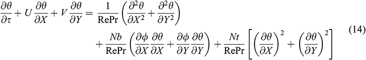
Within the framework of the above-noted assumptions, the governing conservation equations for this model are expressed in dimensional form as follows [9,34–36]:


where  and the descriptions of the physical variables are mentioned in the nomenclature.
2.3 Initial and Boundary Conditions
The appropriate initial and boundary conditions for the above-stated model are as follows:
1) For 

2) For 


2.4 Introduction of Non-Dimensional Variables
The governing differential Eqs. (1)–(5) representing conservation laws are rarely solved using dimensional variables. The common practice is to write these dimensional equations in a non-dimensional form using dimensionless quantities obtained through proper characteristics scales. Writing the conservation equations in non-dimensional forms results in dimensionless numbers that are very useful for performing parametric studies of engineering problems. Again, the use of non-dimensional variables has several advantages. It allows reducing the number of appropriate parameters for the problem considered, revealing the relative magnitude of the various terms in the conservation equation that are less important. This process simplifies the equation to be solved and leaves only the terms of a similar order of magnitude, which results in better numerical accuracy. Besides, the generated solution will apply to all dynamically similar-problems. A dimensional variable is transformed into a non-dimensional one by dividing the variable by a quantity (composed of one or more physical properties) having the same dimension as the original variable. Thus the non-dimensional forms of the governing conservation Eqs. (1)–(5) together with the initial and boundary conditions (6)–(9) are obtained by employing the following dimensionless parameters:
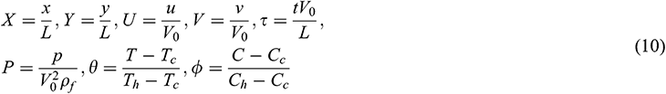
Substituting (10) into (1)–(5), we obtain the dimensionless equations as follows:


The non-dimensional boundary conditions become
1. For  :
:

2. For  :
:


The parameters appeared in (11)–(19) are defined by
 is the aspect ratio of the triangular enclosure,
  is the Prandtl number,
 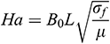 is the Hartmann number,
  is the Reynolds number,
  is the Lewis number,
 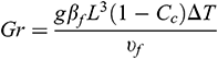 is the Grashof number,
  is the Richardson number,
 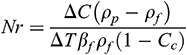 is the buoyancy ratio parameter,
 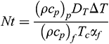 is the thermophoresis parameter, and
  is the Brownian diffusion parameter.
The dimensionless Eqs. (11)–(15) determine the physical parameters that affect the solutions. The role of these parameters on the flow and thermal fields are discussed in the results and discussion section.
The significant physical quantity in this model is the calculation of the average Nusselt number  along the left heated wall. The Nusselt number
  is the ratio of convective to conductive heat transfer across the boundary, and the local Nusselt number is defined by

where  ,
,  is the height of the triangle (the vertical heated wall),
  is the thermal conductivity of the base fluid. The convective heat transfer coefficient of the nanofluid flow
  is defined by

Using the dimensionless variables defined in Eq. (10), the heat transfer coefficient of nanofluid at the left heated wall turns into

Hence, the local Nusselt number for nanofluid at the left heated wall can be expressed as

The average Nusselt number is expressed as follows:

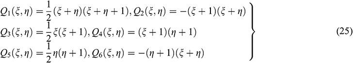
We applied the Galerkin weighted residual-based finite element method (FEM) to solve the governing dimensionless Eqs. (11)–(15) and boundary conditions (17)–(19). A finite element method is a numerical tool that approximates the solution of boundary value problems of partial differential equations. The finite element method exhibits high accuracy of calculation and easily handles complex geometries in engineering problems. In FEM, we construct approximation functions using the weighted-integral technique to find a solution of differential equations. We accomplished this by dividing the whole domain into a set of small sub-domains called finite elements. These elements can be of different types. In 2D problems, we usually use either triangular or quadrilateral shape elements. Besides, in 3D, the most commonly used elements’ shape is tetrahedral or hexahedral. Here, we used six node triangular shape elements for developing the finite element equations. All six nodes are connected with velocities, temperature, and concentration fields, while only the corner nodes are associated with pressure. In the finite element method, the approximate solutions are expressed in terms of the shape (or interpolation) functions, which can be linear or quadratic depending on the number of nodes per element. Also, in 2D problems, the  ,
,  - coordinates (global coordinate) are mapped into
  ,
,  coordinates (or local coordinates), and the shape functions are defined as functions of
  and
and  . Such local coordinates
  are useful in the numerical evaluation of the integration. Now in terms of local coordinates, the quadratic shape functions for the velocities, temperature, and concentration are as follows:
where

and

Also, the linear shape functions for the pressure are as follows:

with the property

and

Again, for the triangular shape element, the coordinates  ,
,  can be represented in terms of nodal coordinates using the same shape functions and this is known as isoparametric representation. Thus, for isoparametric representation, the transformation between
  and
and  is accomplished by a coordinate transformation of the form

In the 2D problem discussed here, each node is permitted to displace along with the two directions,  and
and  Thus, each node has two degrees of freedom. As a result, the number of unknown variables for velocities, temperature, concentration, and pressure is 27 per element, and hence there are 27 degrees of freedom. Thus, in terms of the above-defined shape functions, the approximate solutions of


 and
and  can be expressed as follows:
where 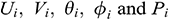 are the corresponding nodal values of the unknown functions.
In the Galerkin weighted residual-based finite element method, the weight functions that we choose are the same as the shape functions that have been used in the approximate solutions (32). Thus employing the Galerkin weighted residual approach on Eqs. (11)–(15) and also using the Gauss’s divergence theorem on the second derivative terms that contain in Eqs. (12)–(15), we get finally, the following finite element equations:

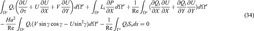


Here,  is the typical triangular element area,
  is the boundary of the element
  ,
,  is the arc length of an infinitesimal line element along the boundary
  ,
,  is the unit outward normal vector on the boundary
  ,
,  and
and  are the outflows from the boundary along the
  and
and  - directions respectively.
  denotes the heat flux normal to the boundary of the element and
  is the sum of heat and mass fluxes which are normal to the boundary of the element
  .
.
We used a three-point Gaussian quadrature formula to evaluate the integrals in the residual Eqs. (33)–(37). Using the Newton-Raphson method, non-linear residual Eqs. (33)–(37) are solved to determine the coefficients of the expansions in Eq. (32). The details of this technique are well documented in the textbook by Reddy et al. [43]. The readers can also consult the work of Uddin et al. [44]. We set  , where
  is the general dependent variable
  , and
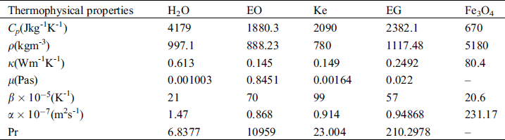
, and  is the number of iteration in order to calculate the error and to determine the convergence of the solution. We tabulated the thermophysical properties of the base fluids and nanoparticles in Tab. 1.
Table 1: Thermo-physical properties of the base fluids and nanoparticles (see [15])
3.1 Test for Grid Independence
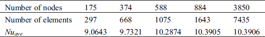
The scrutiny of grid sensitivity on a converged solution is essential for the correct usage of the finite element method. Here, we examined five non-uniform grids named coarse, normal, fine, finer, and extra-fine. Each of them has 297, 668, 1075, 1643, and 7435 number of elements within the resolution field. We have calculated the average Nusselt number ( ) for the afore-said mesh elements and tabulated in Tab. 2 for understanding grid fineness. From Tab. 2, we notice that the values of the average Nusselt number for 1643 and 7435 mesh elements remain almost the same. It indicates that either 1643 or 7435 mesh elements are sufficient to obtain a grid-independent solution. To save run time and memory, we used 1643 mesh elements for numerical computation.
Table 2: Grid sensitivity check for  -water nanofluid when
  ,
,  ,
,  ,
,  ,
,  ,
,  ,
,  , and
, and 
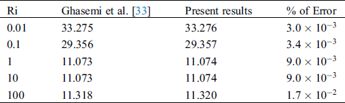
We tallied our simulated results with the work of Ghasemi et al. [33]. They studied a mixed convection flow in a lid-driven right-angled triangular cavity in the absence of mass transfer. They have considered the insulated horizontal wall, hot inclined wall, and uniformly moving cold vertical wall. In Tab. 3, we compared our calculated average Nusselt number with Ghasemi et al. [33] varying Richardson number, Ri. The comparisons show an excellent agreement among the data and inspire us to use the current code.
Table 3: Comparison of average Nusselt numbers  with those of Ghasemi et al. [33] when

 and
and  in the present model
4 Numerical Results and Discussion
In this section, we mainly presented average Nusselt numbers computed for different values of the model parameters. Due to the Brownian diffusion and thermophoresis, it is expected that there is a minimal concentration difference say,  within the flow field. For Fe3O4 nanoparticle with diameter
  , and assuming reference temperature
  , temperature difference
  , the Brownian diffusion and thermophoresis coefficients are calculated as
 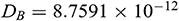 and
and  respectively (see [44,45]). The corresponding values for the other physical parameters are
  ,
,  ,
,  , and
, and  . It is good mention that in nanofluid research using Buongiorno model, the values of the Brownian diffusion parameter
  , thermophoresis parameter, and Lewis number are very poorly determined in a significant number of studies in the open literature (see [46]). In our simulation, we have used the realistic values of the aforesaid-parameters, which make this study unique. For numerical computation, we considered
  ,
,  ,
,  ,
,  ,
,  ,
,  ,
,  ,
,  , and
, and  as default unless otherwise specified.
Figure 2: Streamlines for Fe3O4-water nanofluid for different dimensionless time  when
when  ,
,  ,
,  ,
,  ,
,  ,
,  ,
,  ,
,  and
and 
To explore the time progression of numerical solutions, we have calculated the streamlines of Fe3O4-water nanofluid for different values of the dimensionless time  keeping other model parameter values fixed. We have taken the snapshot of the unsteady solution at
  , 0.1, 1, and 1.5 and depicted in Fig. 2. This series of figures show the time progression of solutions from the transient state to a steady state. We can see that when
  , there are no changes in the structure of streamlines, which means that the solution reached a steady-state. As dimensionless time increases, the fluid flow intensity increases and approaches a steady-state.
Figure 3: Dimensionless time  needed to reach the solution in steady state for different
  when
when  ,
,  ,
,  ,
,  ,
,  ,
,  ,
,  ,
, 
Fig. 3 shows the dimensionless time  needed to reach the solution in a steady-state for different Richardson number
  . We detected that for increasing Richardson’s number the solution requires more time to be in a steady-state. It is because increased Ri weakens inertia force over the buoyancy force as a result of the external driving force, the nanofluid motion diminishes. Hence, the system required more time to be in a steady-state.
Figs. 4(a)–4(c), respectively, illustrate the average Nusselt number  , i.e., the rate of heat transfer from the hot surface (left vertical wall of the cavity) to the nanofluid for different values of the (a) Richardson number
  , (b) Hartmann number
  as well as (c) magnetic field orientation angle
  concerning various dimensionless time
  . The variation in average Nusselt number against dimensionless time shows the evolution of solution from the unsteady-state to the steady-state. The average Nusselt number
  is very-large, near
  , due to the sudden increase in temperature at the vertical wall. The average Nusselt number decreases with time and approaches a steady-state after a certain-time
  . Also, it can be seen that as the Richardson number increases, the average Nusselt number also increases due to the natural convection. From these figures, we observe that higher values of the Hartmann number, as well as the magnetic field inclination angle, forced the solution to reach a steady-state earlier compared to the absence of the magnetic field within the flow domain. We also found that the heat transfer rate decreases with the increase of the values of
  , whereas when the Hartmann number
  , as well as the magnetic field inclination angle, increases, the rate of heat transfer decreases.
Figure 4: (a)–(c) Average Nusselt number for different value of (a)  and
and  , (b)
, (b)  and
and  , (c)
, (c)  and
and  when
when  ,
,  ,
,  ,
,  ,
,  ,
, 
Figure 5: Average Nusselt number for different value of  and
and  when
when  ,
,  ,
,  ,
,  ,
,  ,
,  ,
, 
Fig. 5 shows the average Nusselt number for different Hartmann number  with various values of the Richardson number
  . As clearly seen, for
  , the heat is transferred inside the enclosure by conduction and the convection mode of heat transfer starts when
  . When the Hartmann number is zero (
 ) or when the effect of the magnetic field is absent, the average Nusselt number increases sharply. In this case, the buoyancy force due to the natural convection effect is the only dominant force in the enclosure. When the Hartmann number increases, the Lorentz force becomes energetic and dominates over the buoyancy force that causes a reduction the heat transfer for all considered values of
  . It means that a stronger magnetic field may delay the onset of convection. Thus, the rate of heat transfer can be controlled by controlling the strength of the applied magnetic field.
Figure 6: Average Nusselt number for different values of the magnatic field inclination angle  when
when  ,
,  ,
,  ,
,  ,
,  ,
,  ,
,  , and
, and 
The effects of the orientation of the magnetic field on the average Nusselt number are displayed in Fig. 6. From this figure, we see that  decreases with the increase of
  when
when  , but a further escalation in
  enhances the rate of heat transfer. Thus, we can say that the magnetic field inclination angle, as well as the Hartmann number, significantly controls the heat transfer rate.
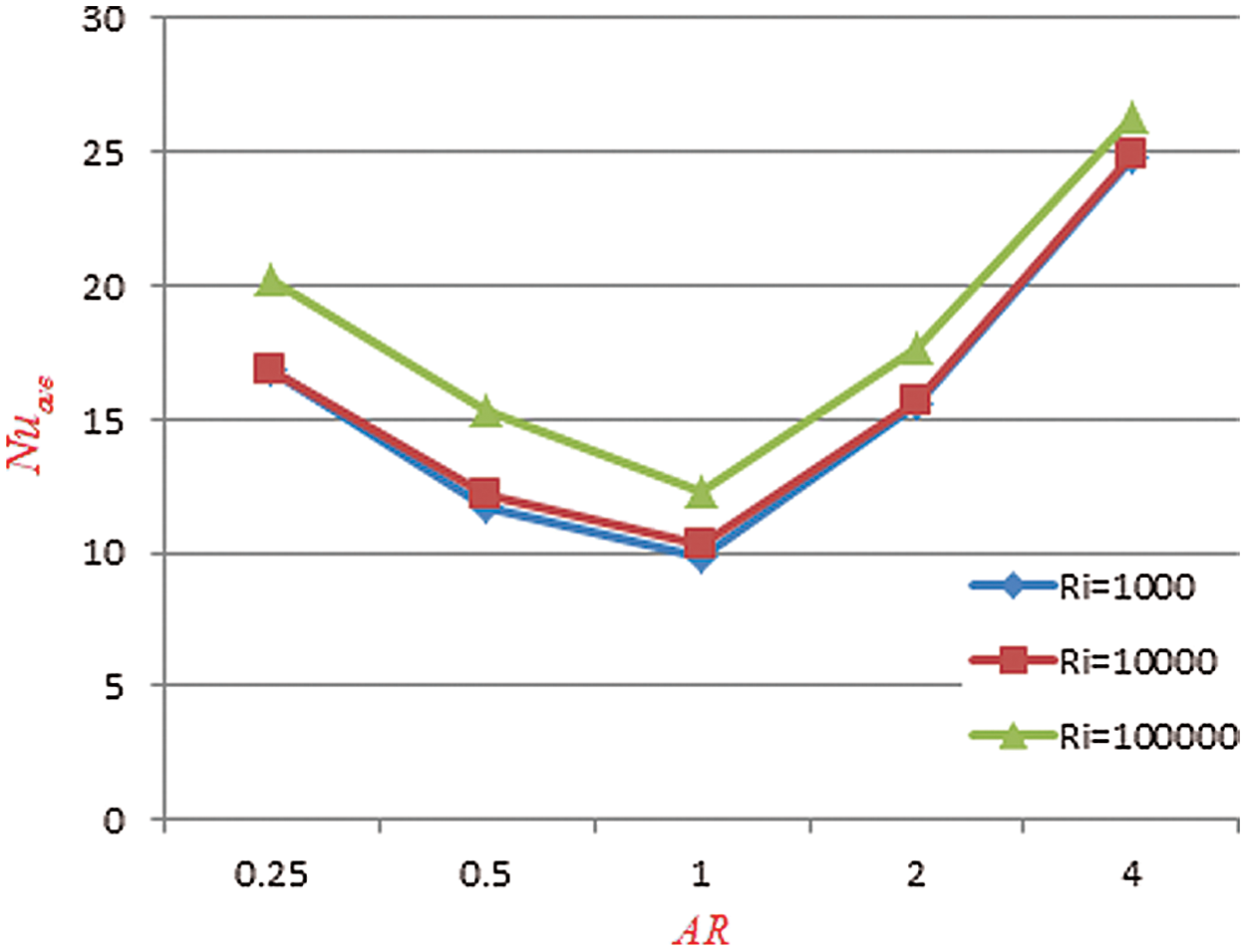
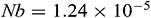
Figure 7: Average Nusselt number for different Richardson number  and different aspect ratios
  when
when  ,
,  ,
,  ,
,  ,
,  ,
,  ,
,  °,
°, 
One of the most critical characteristics of the problem is the change of the aspect ratio ( ) between the height (the vertical-wall) and length (the horizontal wall) of the triangular enclosure. The diagrams in Fig. 7 show the effect of change in the aspect ratio for different Richardson numbers on the average Nusselt number and resulting heat transfer. As the aspect ratio increases, the average Nusselt number decreases for
  . For
. For  , the average Nusselt number increases with the increment of
  for all
  .
.
Figure 8: Dimensionless time  needed to reach the solution in steady state for different Richardson number and different aspect ratios when
  ,
,  ,
,  ,
,  ,
,  ,
,  , and
, and  °
°
We can see from Fig. 8 that changing the aspect ratio has a significant effect on the time required for the solution to reach a steady-state with increasing Richardson number. It is observed from this figure that at the lower value of aspect ratio and for increasing Richardson’s number, the solution needs less time to reach a steady-state. Thus, we may conclude that changing the aspect ratio of the triangular enclosure helps the solution reach a steady-state faster with increasing 
Figure 9: Average Nusselt number for various thermal boundary conditions with different base fluids; H2O, Ke, EG and EO when  ,
,  ,
,  ,
,  , and
, and  . The actual value of the average Nusselt number for EO is divided by 20 to fit within the diagram
In our physical model, we have considered that the vertical wall of the triangular enclosure is uniformly heated ( ). But in reality, this configuration may change depending on the specific applications. Thus, it is essential to study the present model taking into the effects of varying the thermal boundary conditions to a non-uniformly heated wall such as
  and
and  . Consideration of these conditions further eliminates the discontinuity of the temperature at the top corner of the cavity, where there is a hot and cold wall junction. To study these, we have taken into account the effects of different base fluids such as Kerosene (KE), Ethylene Glycol (EG), and Engine Oil (EO) on the heat transfer mechanisms. Fig. 9 displayed the average Nusselt number for various thermal boundary conditions; Case 1:
  , Case 2:
  , and Case 3:
  and for different base fluids (H2O, Ke, EG, EO) considering Fe3O4 nanoparticles when
  ,
,  ,
,  ,
,  , and
, and  . From this figure, we observe that Case1 gives the highest average Nusselt number comparing to the other two-cases for all types of base fluids. On the other hand, the lowest average Nusselt number we recorded for Case 2. The Fe3O4-EO nanofluid gives the higher rate of heat transfer, whereas, Fe3O4-H2O has the lowest rate of heat transfer for all three cases of the thermal boundary conditions.
Figure 10: Average Nusselt number for various thermal boundary conditions with different aspect ratio when  ,
,  ,
,  ,
,  ,
,  ,
,  ,
,  ,
,  °, and
Fig. 10 demonstrates the average Nusselt number for various thermal boundary conditions: Case 1, Case 2, and Case 3 with different aspect ratios. As displayed before, Case 1 gives the highest average Nusselt number comparing to the other two-cases for all values of AR. Besides, for all three cases of the thermal boundary conditions, the average Nusselt number decreases with the increase of the aspect ratio. It indicates that the various thermal boundary conditions at the heated wall do not have a significant influence on the aspect ratio of the triangular enclosure.
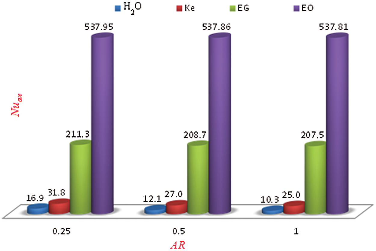
Figure 11: Average Nusselt number for different aspect ratios with various type of base fluids H2O, Ke, EG and EO when  ,
,  ,
,  ,
,  , and
, and  °, and
  . The actual value of the average Nusselt number for EO is divided by 20 to fit within the diagram
The average Nusselt number for different aspect ratios with various types of base fluids (H2O, Ke, EG, and EO) is displayed in Fig. 11. As stated before, the average Nusselt number decreases with the rise of the aspect ratio for all four types of base fluids. Besides, as we observed in Fig. 9, Fe3O4-EO nanofluid gives the highest rate of heat transfer, whereas Fe3O4-H2O has the lowest heat transfer. So changing the aspect ratio leads to the same trend of heat transfer for different types of base fluids.
In this work, we numerically studied the problem of unsteady natural convection flow and heat transfer in a lid-driven right-angle triangular shaped enclosure filled with Fe3O4 nanoparticles in four different types of base fluids such as water, kerosene, ethylene glycol, and engine oil in the presence of an inclined magnetic field. The model used for the binary nanofluid incorporates the effects of Brownian motion and thermophoresis. The influence of changing the thermal boundary conditions of the enclosure was also investigated, taken into account different aspect ratios of the cavity. Furthermore, we analyzed the time evolution of the solution from unsteady to the steady-state. In the physical model, the effects of the different model parameters such as Richardson number  Hartmann number
  the inclination angle (
 ) of the magnetic field, aspect ratio (AR), and various thermal boundary conditions on the average Nusselt number were investigated in details and discussed their physical significance. From the numerical simulations, we found that a strong magnetic field may suppress the convection mechanisms in nanofluids, as a consequence rate of heat transfer decreases. The magnetic field orientation significantly controls the rate of heat transfer in nanofluids. For the higher value of
  , the heat transfer rate decreases through lower-values of
  ; but increases through the large-value of
  . The higher
  confirms better heat transfer through convection than conduction. The heat transfer rate of Fe3O4-EO nanofluid for a uniformly heated wall case is 537.81%, whereas the corresponding rate for the Fe3O4-EG, Fe3O4-Ke and Fe3O4-H2O nanofluids are 207.45%, 25.03%, and 10.25%, respectively. Again, the heat transfer rate of Fe3O4-EO nanofluid for non-uniformly heated wall case (parabolic case) is 91.19%, whereas the corresponding rates for the Fe3O4-EG, Fe3O4-Ke, and Fe3O4-H2O nanofluids are 34.08%, 3.99%, and 1.49%, respectively. Finally, the heat transfer rate of Fe3O4-EO nanofluid for a non-uniformly heated wall case (sinusoidal case) is 347.51%,whereas the corresponding rates for the Fe3O4-EG, Fe3O4-Ke, and Fe3O4-H2O nanofluids are 134.59%, 16.81%,and 8.15%, respectively. Thus, we can conclude that the heat transfer rate strongly depends on the types of nanofluids as well as the types of boundary conditions.
Acknowledgement: M. M. Rahman is grateful to the Sultan Qaboos University for the internal research grant.
Funding Statement: This work was supported by IG/SCI/MATH/20/03.
Conflicts of Interest: The authors declare that there is no conflict of interest.
1. Bayomy, A., Saghir, M. Z., Yousefi, T. (2016). Electronic cooling using water flow in aluminum metal foam heat sink: Experimental and numerical approach. International Journal of Thermal Sciences, 109, 182–200. DOI 10.1016/j.ijthermalsci.2016.06.007. [Google Scholar] [CrossRef]
2. Choi, S. (1995). Enhancing thermal conductivity of fluids with nanoparticles. In: Signier, D. A., Wang, H. P. (eds.Development and applications of non-Newtonian flows. ASME FED, vol. 231/MD1995; 66, pp. 99–105. [Google Scholar]
3. Sundar, L. S., Naik, M. T., Sharma, K. V., Singh, M. K., Reddy, T. C. S. (2012). Experimental investigation of forced convection heat transfer and friction factor in a tube with Fe3O4 magnetic nanofluid. Experimental Thermal and Fluid Science, 37, 65–71. DOI 10.1016/j.expthermflusci.2011.10.004. [Google Scholar] [CrossRef]
4. Bayomy, A. M., Saghir, M. Z. (2017). Experimental study of using γ-Al2O3-water nanofluid flow through aluminum foam heat sink: Comparison with numerical approach. International Journal of Heat and Mass Transfer, 107, 181–203. DOI 10.1016/j.ijheatmasstransfer.2016.11.037. [Google Scholar] [CrossRef]
5. Saghir, M. Z., Welsford, C., Thanapathy, P., Bayomy, A. M., Delisle, C. (2020). Experimental measurements and numerical computation of nano heat transfer enhancement inside a porous material. Journal of Thermal Science and Engineering Applications, 12(1), 1023. DOI 10.1115/1.4041936. [Google Scholar] [CrossRef]
6. Alhajaj, Z., Bayomy, A. M., Saghir, M. Z., Rahman, M. M. (2020). Flow of nanofluid and hybrid fluid in porous channels: Experimental and numerical approach. International Journal of Thermofluids, 1–2, 100016. DOI 10.1016/j.ijft.2020.100016. [Google Scholar] [CrossRef]
7. Ho, C. J., Chen, W. C. (2013). An experimental study on thermal performance of Al2O3/water nanofluid in a minichannel heat sink. Applied Thermal Engineering, 50(1), 516–522. DOI 10.1016/j.applthermaleng.2012.07.037. [Google Scholar] [CrossRef]
8. Nabil, M. F., Azmi, W. H., Hamid, K. A., Mamat, R., Hagos, F. Y. (2017). An experimental study on the thermal conductivity and dynamic viscosity of TiO2-SiO2 nanofluids in water: Ethylene glycol mixture. International Communications in Heat and Mass Transfer, 86, 181–189. DOI 10.1016/j.icheatmasstransfer.2017.05.024. [Google Scholar] [CrossRef]
9. Buongiorno, J. (2006). Convective transport in nanofluids. Journal of Heat Transfer, 128(3), 240–250. DOI 10.1115/1.2150834. [Google Scholar] [CrossRef]
10. Wang, X., Xu, X., Choi, S. U. (1999). Thermal conductivity of nanoparticle-fluid mixture. Journal of Thermophysics and Heat Transfer, 13(4), 474–480. DOI 10.2514/2.6486. [Google Scholar] [CrossRef]
11. Xuan, Y., Li, Q. (2003). Investigation on convective heat transfer and flow features of nanofluids. Journal of Heat Transfer, 125(1), 151–155. DOI 10.1115/1.1532008. [Google Scholar] [CrossRef]
12. Eastman, J. A., Phillpot, S. R., Choi, S. U. S., Keblinski, P. (2004). Thermal transport in nanofluids. Annual Review Materials Research, 34(1), 219–246. DOI 10.1146/annurev.matsci.34.052803.090621. [Google Scholar] [CrossRef]
13. Jalali, H., Abbassi, H. (2020). Analysis of the influence of viscosity and thermal conductivity on heat transfer by Al2O3-water nanofluid. Fluid Dynamics & Materials Processing, 16(2), 181–198. DOI 10.32604/fdmp.2020.07804. [Google Scholar] [CrossRef]
14. Khanafer, K., Vafai, K., Lightstone, M. (2003). Buoyancy-driven heat transfer enhancement in a two-dimensional enclosure utilizing nanofluids. International Journal of Heat and Mass Transfer, 46(19), 3639–3653. DOI 10.1016/S0017-9310(03)00156-X. [Google Scholar] [CrossRef]
15. Oztop, H. F., Abu-Nada, E. (2008). Numerical study of natural convection in partially heated rectangular enclosures filled with nanofluids. International Journal of Heat and Fluid Flow, 29(5), 1326–1336. DOI 10.1016/j.ijheatfluidflow.2008.04.009. [Google Scholar] [CrossRef]
16. Chamkha, A. J. (2002). Hydromagnetic combined convection flow in a vertical lid-driven cavity with internal heat generation or absorption. Numerical Heat Transfer, Part A: Applications, 41(5), 529–546. DOI 10.1080/104077802753570356. [Google Scholar] [CrossRef]
17. Rahman, M. M., Alim, M. A., Sarker, M. M. A. (2010). Numerical study on the conjugate effect of joule heating and magneto-hydrodynamics mixed convection in an obstructed lid-driven square cavity. International Communications in Heat and Mass Transfer, 37(5), 524–534. DOI 10.1016/j.icheatmasstransfer.2009.12.012. [Google Scholar] [CrossRef]
18. Malleswaran, A., Sivasankaran, S. (2016). A numerical simulation on MHD mixed convection in a Lid-driven cavity with corner heaters. Journal of Applied Fluid Mechanics, 9(1), 311–319. DOI 10.18869/acadpub.jafm.68.224.22903. [Google Scholar] [CrossRef]
19. Al Kalbani, K. S., Alam, M. S., Rahman, M. M. (2016). Finite element analysis of unsteady natural convective heat transfer and fluid flow of nanofluids inside a tilted square enclosure in the presence of oriented magnetic field. American Journal of Heat and Mass Transfer, 3(3), 186–224. [Google Scholar]
20. Al Kalbani, K. S., Rahman, M. M., Alam, S., Al-Salti, N., Eltayeb, I. A. (2017). Buoyancy induced heat transfer flow inside a tilted square enclosure filled with nanofluids in the presence of oriented magnetic field. Heat Transfer Engineering, 39(6), 511–525. DOI 10.1080/01457632.2017.1320164. [Google Scholar] [CrossRef]
21. Al Balushi, L. M., Rahman, M. M. (2019). Convective heat transfer utilizing magnetic nanoparticles in the presence of a sloping magnetic field inside a square enclosure. Journal of Thermal Science and Engineering Applications, 11(4), 99. DOI 10.1115/1.4044120. [Google Scholar] [CrossRef]
22. Al Balushi, L. M., Rahman, M. M. (2020). Impacts of heat flux distribution, sloping magnetic field and magnetic nanoparticles on the natural convective flow contained in a square cavity. Fluid Dynamics & Material Processing, 16(3), 441–463. DOI 10.32604/fdmp.2020.08551. [Google Scholar] [CrossRef]
23. Koseff, J. R., Prasad, A. K. (1984). The lid-driven cavity flow: A synthesis of quantitative and qualitative observations. Journal of Fluids Engineering, 106(4), 390–398. DOI 10.1115/1.3243136. [Google Scholar] [CrossRef]
24. Flack, R. D., Konopnicki, T., Rooke, J. H. (1979). The measurement of natural convective heat transfer in triangular enclosures. Journal of Heat Transfer, 101, 770–772. [Google Scholar]
25. Flack, R. D. (1980). The experimental measurement of natural convection heat transfer in triangular enclosures heated or cooled from below. Journal of Heat Transfer, 102(4), 770–772. DOI 10.1115/1.3244389. [Google Scholar] [CrossRef]
26. Akinsete, V. A., Coleman, T. A. (1982). Heat transfer by steady laminar free convection in triangular enclosures. International Journal of Heat and Mass Transfer, 25(7), 991–998. DOI 10.1016/0017-9310(82)90074-6. [Google Scholar] [CrossRef]
27. Ridouane, E. I., Campo, A., Chang, J. Y. (2005). Natural convection patterns in right-angled triangular cavities with heated vertical sides and cooled hypotenuses. Journal of Heat Transfer, 127(10), 1181–1186. DOI 10.1115/1.2033903. [Google Scholar] [CrossRef]
28. Varol, Y., Oztop, H. F., Varol, A. (2007). Effects of thin fin on natural convection in porous triangular enclosures. International Journal of Thermal Sciences, 46(10), 1033–1045. DOI 10.1016/j.ijthermalsci.2006.11.001. [Google Scholar] [CrossRef]
29. Basak, T., Aravind, G., Roy, S. (2009). Visualization of heat flow due to natural convection within triangular cavities using Bejan’s heatline concept. International Journal of Heat and Mass Transfer, 52(11–12), 2824–2833. DOI 10.1016/j.ijheatmasstransfer.2008.10.034. [Google Scholar] [CrossRef]
30. Yesiloz, G., Aydin, O. (2013). Laminar natural convection in right-angled triangular enclosures heated and cooled on adjacent walls. International Journal of Heat and Mass Transfer, 60, 365–374. DOI 10.1016/j.ijheatmasstransfer.2013.01.009. [Google Scholar] [CrossRef]
31. Triveni, M. K., Panua, R. (2018). Numerical study of natural convection in a right triangular enclosure with sinusoidal hot wall and different configurations of cold wall. Fluid Dynamics and Materials Processing, 14(1), 1–21. [Google Scholar]
32. Ghasemi, B., Aminossadati, S. M. (2010). Brownian motion of nanoparticles in a triangular enclosure with natural convection. International Journal of Thermal Sciences, 49(6), 931–940. DOI 10.1016/j.ijthermalsci.2009.12.017. [Google Scholar] [CrossRef]
33. Ghasemi, B., Aminossadati, S. M. (2010). Mixed convection in a lid-driven triangular enclosure filled with nanofluids. International Communications in Heat and Mass Transfer, 37(8), 1142–1148. DOI 10.1016/j.icheatmasstransfer.2010.06.020. [Google Scholar] [CrossRef]
34. Rahman, M. M., Alam, M. S., Al-Salti, N., Eltayeb, I. A. (2016). Hydromagnetic natural convective heat transfer flow in an isosceles triangular cavity filled with nanofluid using two-component nonhomogeneous model. International Journal of Thermal Sciences, 107, 272–288. DOI 10.1016/j.ijthermalsci.2016.04.009. [Google Scholar] [CrossRef]
35. Rahman, M. M. (2016). Influence of oriented magnetic field on natural convection in an equilateral triangular enclosure filled with water-and kerosene-based ferrofluids using a two-component nonhomogeneous thermal equilibrium model. Cogent Physics, 3(1), 1234662. [Google Scholar]
36. Rahman, M. M. (2018). Heat transfer in Fe3O4-H2O nanofluid contained in a triangular cavity under a sloping magnetic field. Sultan Qaboos University Journal for Science, 23(1), 56–67. DOI 10.24200/squjs.vol23iss1pp56-67. [Google Scholar] [CrossRef]
37. Azam, M., Khan, M., Alshomrani, A. S. (2017). Unsteady radiative stagnation point flow of MHD Carreau nanofluid over expanding/contracting cylinder. International Journal of Mechanical Sciences, 130, 64–73. DOI 10.1016/j.ijmecsci.2017.06.010. [Google Scholar] [CrossRef]
38. Azam, M., Khan, M. (2017). Unsteady heat and mass transfer mechanisms in MHD Carreau nanofluid flow. Journal of Molecular Liquids, 225, 554–562. DOI 10.1016/j.molliq.2016.11.107. [Google Scholar] [CrossRef]
39. Azam, M., Shakoor, A., Rasool, H. F., Khan, M. (2019). Numerical simulation for solar energy aspects on unsteady convective flow of MHD Cross nanofluid: A revised approach. International Journal of Heat and Mass Transfer, 131, 495–505. DOI 10.1016/j.ijheatmasstransfer.2018.11.022. [Google Scholar] [CrossRef]
40. Azam, M., Xu, T., Shakoor, A., Khan, M. (2020). Effects of Arrhenius activation energy in development of covalent bonding in axisymmetric flow of radiative-Cross nanofluid. International Communications in Heat and Mass Transfer, 113, 104547. DOI 10.1016/j.icheatmasstransfer.2020.104547. [Google Scholar] [CrossRef]
41. Azam, M., Xu, T., Khan, M. (2020). Numerical simulation for variable thermal properties and heat source/sink in flow of Cross nanofluid over a moving cylinder. International Communications in Heat and Mass Transfer, 118, 104832. DOI 10.1016/j.icheatmasstransfer.2020.104832. [Google Scholar] [CrossRef]
42. Uddin, M. J., Rahman, M. M. (2020). Heat transportation in Copper Oxide-water nanofluid filled triangular cavities. International Journal of Heat and Technology, 38(1), 106–124. DOI 10.18280/ijht.380112. [Google Scholar] [CrossRef]
43. Reddy, J. N., Gartling, D. K. (2010). The finite element method in heat transfer and fluid dynamics, 3rd Edition. Boca Raton, Florida: CRC Press. [Google Scholar]
44. Uddin, M. J., Rahman, M. M. (2018). Finite element computational procedure for convective flow of nanofluids in an annulus. Thermal Science and Engineering Progress, 6, 251–267. DOI 10.1016/j.tsep.2018.04.011. [Google Scholar] [CrossRef]
45. Uddin, M., Kalbani, K. S. A., Rahman, M. M., Alam, M. S., Al-Salti, N. et al. (2016). Fundamentals of nanofluids: Evolution, applications and new theory. Journal of Biomathematics and Systems Biology, 2(1), 1–32. [Google Scholar]
46. Myers, T. G., Ribera, H., Cregan, V. (2017). Does mathematics contribute to the nanofluid debate? International Journal of Heat and Mass Transfer, 111, 279–288. DOI 10.1016/j.ijheatmasstransfer.2017.03.118. [Google Scholar] [CrossRef]
 | This work is licensed under a Creative Commons Attribution 4.0 International License, which permits unrestricted use, distribution, and reproduction in any medium, provided the original work is properly cited. |