Materials Processing
| Fluid Dynamics & Materials Processing |
DOI: 10.32604/fdmp.2021.010528
ARTICLE
Experimental and Numerical Analysis of Surface Magneto-Hydrodynamic Propulsion Induced by NdFeB Magnets
1College of Automation, Nanjing University of Science and Technology, Nanjing, 210094, China
2Nanjing Yue Bo Power System Co., Ltd., Nanjing, 210094, China
*Corresponding Author: Zongkai Liu. Email: kfliukai@126.com
Received: 08 March 2020; Accepted: 29 January 2021
Abstract: The so-called surface Magneto-hydro-dynamic (MHD) propulsion relies on the Lorentz force induced in weak electrolyte solutions (such as seawater or plasma) by NdFeB Magnets. The Lorentz force plays an important role in such dynamics as it directly affects the structures of flow boundary layers. Previous studies have mainly focused on the development of such boundary layers and related fluid-dynamic aspects. The main focus of the present study is the determination of electromagnetic field distributions around the propulsion units. In particular dedicated experiments and numerical simulations (based on the finite volume method) are conducted considering a NACA0012 airfoil immersed in seawater. The results show that, along the propulsion unit, the field strength undergoes a rapid attenuation in the direction perpendicular to the wall.
Keywords: Vector finite element method; edge element method; NdFeB magnet; Lorentz force
Active fluid control is typically used to mitigate the drag force and suppress the noise produced by underwater weapons. Active flow boundary layer control can be based on physical mechanisms such as vortex suppression, separation postponement, transition delay, and velocity adjustment, in the turbulence boundary layer. Electrically conducting fluids (e.g., seawater) can be controlled using the Lorentz force. This may be regarded as a novel and very promising active fluid control mode. The Lorentz force can be generated along different directions over a body; thereby, its outer surface can be used as the working surface of a propeller. The process by which the Lorentz force propels a body is called electromagnetic fluid surface propulsion. One of the advantages associated with magneto-hydro-dynamic MHD control or propellers is the possibility to exert a flexible control directly on the fluid boundary layer by only adjusting the applied voltage [1,2]. Furthermore, moving parts requiring interactions between an actuator and the surrounding fluid are not needed.
Gailitis [3], with the help of an assistant, alternately arranged the strip magnetic poles and electrodes adjacently in parallel. This arrangement forms an electromagnetic actuator. Thereafter, the electromagnetic actuator was immersed in a weak electrolyte solution, which should be prepared according to the sea water conductivity. The interaction between the electric and magnetic fields can produce the Lorentz force, parallel to the magnetic or electrical poles. In previous studies, the flow field structures around the wall Lorentz force were analyzed through numerical simulation and experiments [4]. Globally, researchers have proposed using stripes of electrodes and magnets formed an electromagnetic actuator to prevent boundary layer growth, reduce skin friction, suppress vortices, and postpone flow separation [5,6].
With the continuous development of new technological materials and superconducting technology researchers can obtain a stronger magnetic field more easily, which can establish a sufficiently large electromagnetic field; thus, the electromagnetic fluid surface propulsion can be realized [7,8]. Electromagnetic fluid surface propulsion implies that the Lorentz force can be applied as the driving force generated over the outer surface of the submarine. This method has a certain guiding significance for optimizing the overall outer structure of the submarine and improving the submarine’s propulsion efficiency [9–11].
In addition to using sonars, in future battlefields, the accurate location of submarines can be detected using electromagnetic fields [12]. Seawater is an electrically conducting fluid, and electromagnetic propulsion devices can be used for practical applications. In this work, we discuss the distribution and penetration characteristics of electric fields, magnetic fields, and the Lorentz force around the electromagnetic propulsion unit in seawater. Moreover, owing to the high relative dielectric constant of seawater, electromagnetic fields require a large magnetic field energy propagating through seawater. Therefore, to assess the actual magnetic field strength, further studies should be conducted to improve the electromagnetic safety for underwater navigation and reduce the probability of being electromagnetic field detected by the enemy’s detection equipment. It is necessary to evaluate the electromagnetic safety before the MHD propulsion units are practically applied to underwater navigation systems.
Previous studies on electromagnetic actuators have focused on establishing certain macroscopic mathematical models [13]. Although these efforts can reflect the effects of the Lorentz force and flow fields to a certain extent, few studies have quantitatively analyzed the field strength around the electromagnetic actuator and the electromagnetic environment characteristics in a particular medium, such as seawater. Therefore, in this paper, Section 3 presents the numerical method used for simulation. Section 4 presents the numerical results of investigation of the field strength distribution characteristics above the electromagnetic propulsion unit in seawater. Section 5 describes the simplified electromagnetic field mathematical model. Section 6 presents the numerical and experimental results of flow field evolution comparisons under the Lorentz force control at Reynolds number (Re) = 2000.
2 Structure of the Electromagnetic Propulsion Unit
The electromagnetic propulsion unit used in the numerical simulation was designed with the general geometric characteristics, as shown in Fig. 1. Stripes of eight electrodes and magnetic poles (4 pairs) are alternately arranged in parallel on the surface of an insulator substrate. During the numerical simulation of the electromagnetic field, the coordinate origin was selected at the center of the left edge and maintained 1 mm above the upper surface of the unit. The x- and z-axis are parallel to the horizontal and electromagnetic pole directions of the model, respectively, and the y-axis points directly to the upward direction.
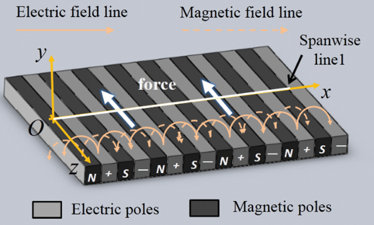
Figure 1: Structure of the electromagnetic propulsion unit
Four white normal lines in the center and one horizontal spanwise line are marked, as shown in Fig. 1. The field strength along some of these lines will be discussed. The four white normal lines in the center, 160 mm in length, start from the center points that the starting points remain 1 mm above the center of the N, –, S, and + poles, repectively. The horizontal spanwise line 1 is maintained 1 mm away from the surface and has a length of 70 mm. The black solid curves and dotted curves represent the electric and magnetic field lines, respectively. The two large arrows along the electric and magnetic pole strips denote the direction of the induced Lorentz force.
3 Numerical Methods and Boundary Conditions
The magnetic induction H (A/m) can be transformed from the magnetic induction value B using
where
Based on Maxwell’s equations, the mutual conversion relationship between the electric field E and magnetic field B can be expressed as follows:
From Ohm’s law, we obtain
where J, U,
Eqs. (2) and (3) are the common electromagnetic field equations. However, in this work, the voltage can be adjusted with time. For time-varying electromagnetic fields, Eqs. (2) and (3) can be rewritten as vector wave Eqs. (5) and (6). The distributions of the electric field, magnetic field, and electromagnetic force around the actuator are analyzed using the finite element method (Vector finite element method-edge element method) [14].
Here,
where Vm denotes the volume of the different dielectric layers. To realize the spatial dispersion of
where
Here,
To solve Eq. (11), we applied Rayleigh-Ritz method, where F(E) is considered as a partial derivative with respect to each of the unknown divided edge fields, and then, the equations are set to zero. Thus, the eigenvalue equations can be obtained, and eigenvalue
Practically, the electromagnetic parameters are not constants for different latitudes of the global ocean. Most of these values change with the local seawater salinity and temperature. Seawater is a non-ferromagnetic substance, and its magnetic permeability is approximately equal to the permeability of vacuum. The conductivity of seawater ranges from 3 to 5 S/m. At 17°C, the standard seawater conductivity ranges between 4.54 S/m and 4.82 S/m, and the relative dielectric constant is approximately 81.
There are two types of ocean background electromagnetic fields: natural and induced. The natural electromagnetic field primarily refers to the geomagnetic field, which varies based on the earth’s latitude. The earth’s magnetic field in the north or south poles can reach an extreme value of approximately
In this numerical simulation, the overall electromagnetic propeller unit length, width, and height were 160 mm, 120 mm, and 9 mm, respectively. The electrode and magnetic pole stripes were of the same size; the length, width, and thickness are 120 mm, 2 mm, and 0.1 mm, respectively. Glass_PTFEreinf was used as the substrate material, neodymium iron boron magnetic was used as the magnetic pole, and copper was utilized as the electrode. NdFeB magnet remanence was 1 T, the coercive force in this work was −900000 A/m, and the positive and negative electrode voltages were selected as +10 V and −10 V, respectively.
4 Field Strength Distribution Characteristics
Fig. 2 shows the surface voltage distribution of the propulsion unit. It can be observed that the voltage peak alternates with the positive and negative electrodes on the surface. The maximum positive voltage on the surface of the positive electrode (indicated by red) is approximately 9–10 V, and the minimum negative voltage on the surface of the negative electrode ranges from approximately −9 V to −10 V. However, the boundaries of these values are not clear. This is because the seawater and surrounding magnets are the conductors; thus, the voltage can penetrate the adjacent magnetic poles or seawater.
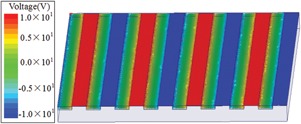
Figure 2: Permeability regions of electrode voltage
Fig. 3 displays the spanwise voltage distribution curve along the horizontal white spanwise horizontal line 1 showing in Fig. 1. The
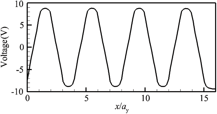
Figure 3: Voltage distribution curve along the spanwise horizontal line 1
Fig. 4 shows the voltage and electric field change with the wall-normal direction above the positive electrode center (the white center normal line in Fig. 1). Fig. 4 shows that the voltage decays rapidly with the increase in the wall-normal distance from the positive center surface. The voltage is approximately 9 V at a 1 mm distance (
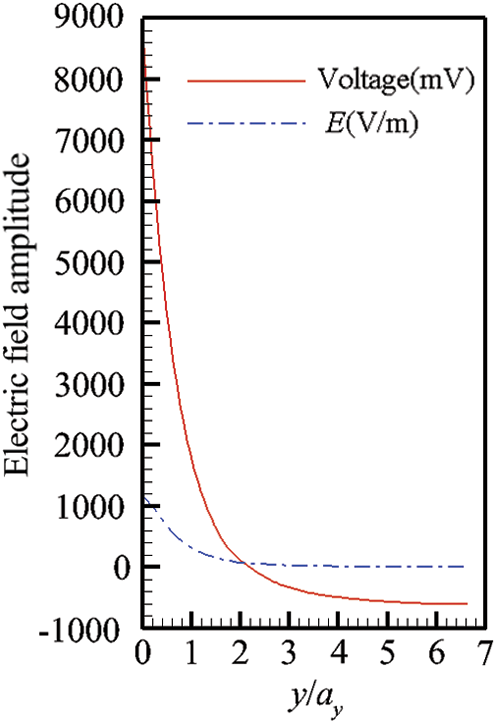
Figure 4: Voltage and E field distributions along the wall-normal lines from the positive electric pole center
Fig. 5 shows the permeability regions of the magnetic induction field around the propulsion unit. It can be observed that near the magnetic pole edges, the magnetic induction intensity is significantly larger than those at the central zones. Moreover, the magnetic induction lines emerge from the N pole and end to the S pole outside the magnet (as shown in Fig. 1). The inward arrow on the surface of the S pole indicates the magnetic induction line entering the S pole, and the other end of the line emerges from the N pole.
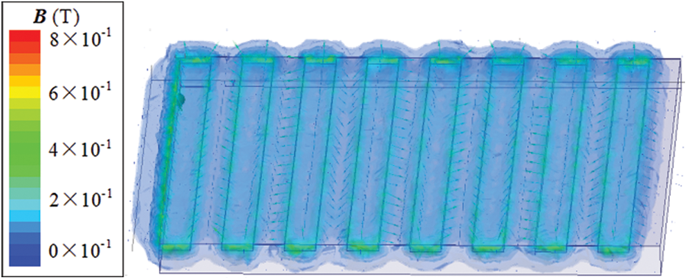
Figure 5: Permeability regions of magnetic induction field
Fig. 6 illustrates the spanwise distribution of magnetic induction strength along line 1 parallel to the surface of the propulsion unit. It can be observed that the magnetic induction along line 1 exhibits a series of sharp fluctuations, and the field strength peaks can reach approximately 0.64–0.7 T, which can be detected at
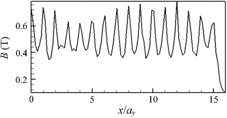
Figure 6: Magnetic induction strength distribution curve along spanwise line 1
Fig. 7 depicts the Lorentz force distribution along line 1, which shows that the near-wall Lorentz force is perpendicular to the arrangement direction of the poles, ranging from 1500–7500 N/m3. Similar to the magnetic induction distribution, the Lorentz force exhibits several significant fluctuations with the change in the N, +, S, and – poles. Compared with Figs. 3 and 5, it can be observed that both the magnetic induction field and Lorentz force can reach the maximum peak values at the same x/ay positions; however, the Lorentz force maximum values do not show evident correlation with the voltage distribution. Figs. 6 and 7 demonstrate sixteen peaks of the force and magnetic induction strength, respectively, which are majorly caused by the boundary effect of magnetic poles.
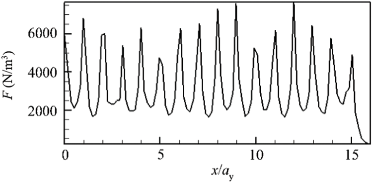
Figure 7: Electromagnetic force distribution curve along line 1
Fig. 8 illustrates the magnetic field and magnetic induction strength curves above the N pole center of the propulsion unit. It can be observed from Fig. 8 that, at the near-wall surface, the magnetic field strength has a maximum value and is continuously attenuated as the normal distance increases. It decays to 30 kA/m when
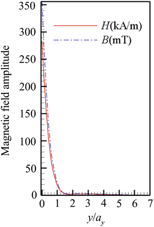
Figure 8: Magnetic field strength changes along the wall-normal line starting from the N pole center
Fig. 9 presents two distribution curves of the Lorentz force along the wall-normal direction above the N and S magnet poles. From the figure, the maximum Lorentz force is exhibited at the wall surface, which is approximately 1.6 and 1.8 kN/m3 at the N and S poles’ surfaces, respectively. It decays slowly in the normal direction of the N or S pole. Furthermore, the electromagnetic force primarily acts at
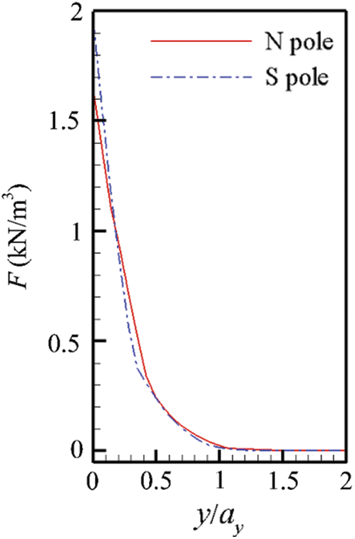
Figure 9: Lorentz force strength changes along the wall-normal line from the N and S pole centers
It can be observed from the above figures that, in seawater, the propeller unit that can produce the Lorentz force exhibits a periodic variation along the span direction and an exponential decay in the wall-normal direction. For the electromagnetic environment characteristics of electromagnetic propulsion units in seawater, the N and S poles are adjacent and alternately arranged, thereby the magnetic field lines originated from the N poles will ended to the nearest S poles forming a short loop of the magnetic field. Therefore, the magnetic lines from N to S are not too long on the surface of the propulsion device without an evident magnetic leakage phenomenon. While
5 Simplified Mathematical Model of the Electromagnetic Field
This study primarily focuses on the electromagnetic field vector wave equations, which consider the fluctuation of the electromagnetic fields and their mutual intercoupling relationships. However, in the numerical simulation of the flow field, we should further simplify the above equations to better analyze the interaction mechanism between the electromagnetic field and weak electrolyte solution. In addition, as seawater is a weak electrolyte solution, the fluctuation information of electric and magnetic fields over time is excluded here.
A simplified mathematical model is required in the numerical calculation of the flow field evolution under the action of the Lorentz force. Since the research object is a weakly conductive fluid (seawater) and is electrically neutral, during the numerical investigation using Eqs. (2) and (3),
The electric and magnetic fields are irrotational; thus, they can be denoted as the electric potential function U and magnetic potential function
To obtain U and
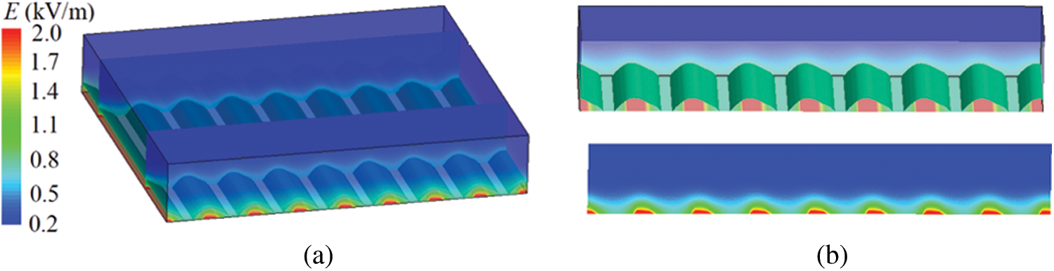
Figure 10: The electric field distributions around the actuator (a) Whole view, (b) Section view
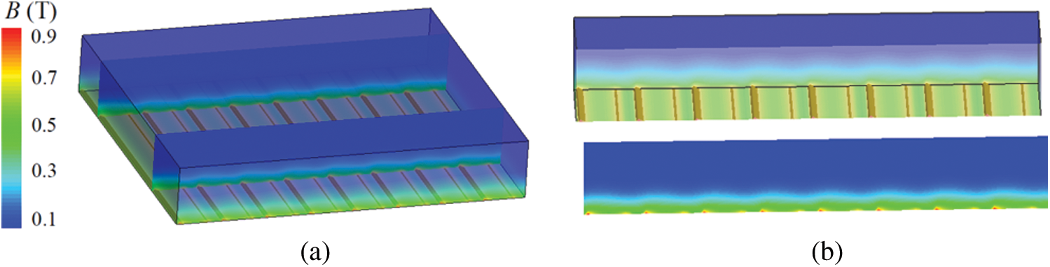
Figure 11: The magnetic induction field distributions around the actuator (a) Whole view, (b) Section view
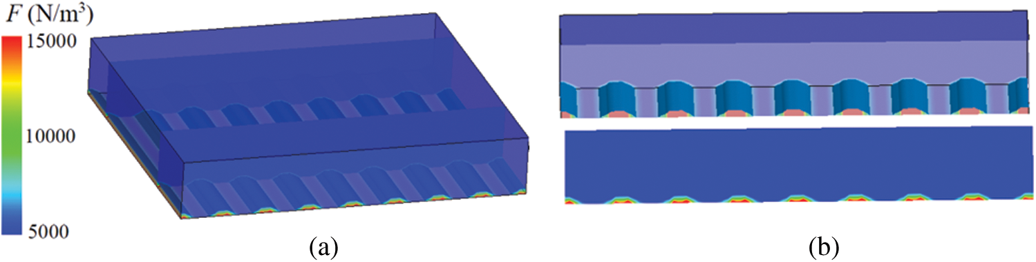
Figure 12: Lorentz force distributions around the actuator (a) Whole view, (b) Section view
Because the distribution of the Lorentz force along the normal direction plays an important role in flow control and in the 2D model or simple 3D model, the crosswise evolution characteristics of the Lorentz force and the influence of the induction term for the entire Lorentz force can be neglected. In the electromagnetic fluid control, the distribution of this force is usually simplified as an exponential function that only changes with the wall-normal distance:
where N denotes the dimensionless Lorentz force action parameter, which can be expressed as
where
6 Numerical and Experimental Comparisons
To understand the application of electromagnetic fluid surface propulsion or control, the structure and evolution characteristics of the flow field around the hydrofoil influenced by the streamwise Lorentz force are analyzed according to experiments and numerical simulation. The results of the flow around the rudder plane are presented in Liu et al. [18]. The hydrofoil structure and its experimental model are presented in Figs. 13a and 13b. The experiment was conducted in a rotating water tank. Potassium permanganate microtubules were used to mark the fluid flow paths. The conductive fluid density was 1003 kg/m3, electrical conductivity was 10 S/m, electrode voltage was 8 V, current density was 1210 A/m2, and Re was 2000. The incoming flow velocity and the chord length of the hydrofoil are 1 m/s and 0.1 m, respectively.
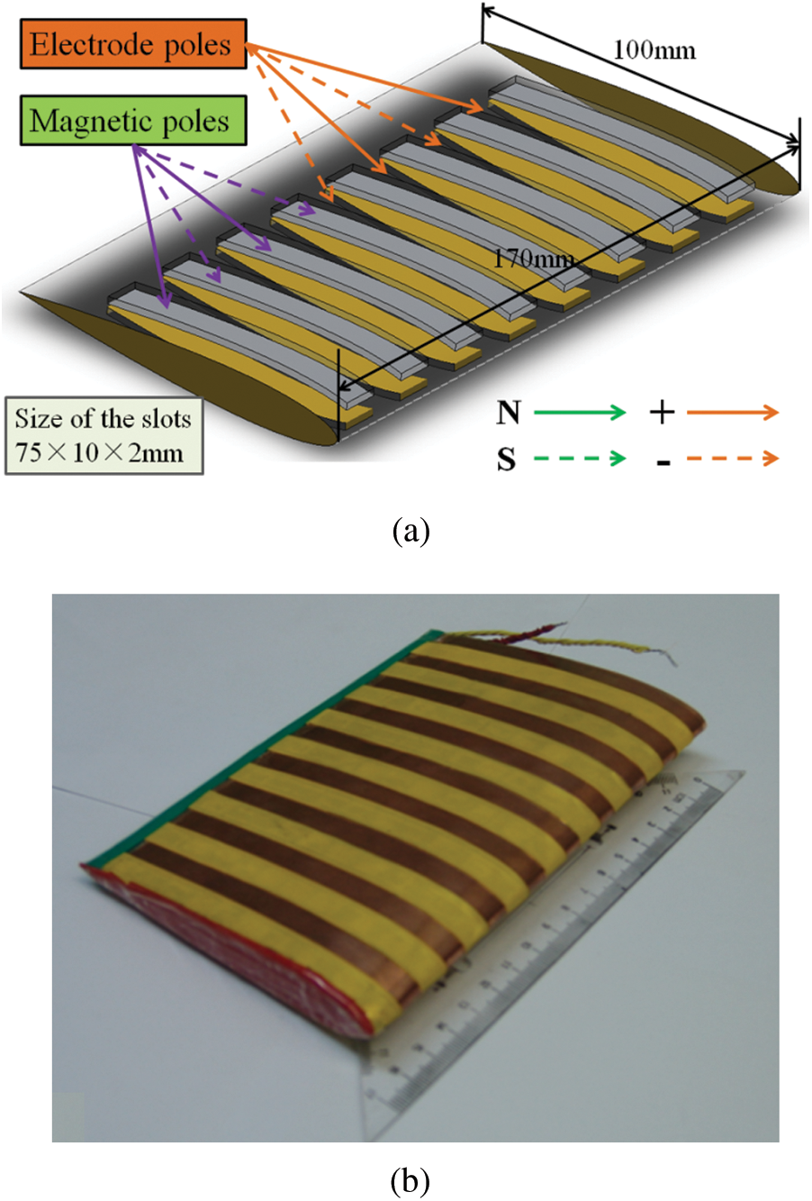
Figure 13: (a) The hydrofoil structure chart and (b) The experimental model covered by the actuators
Figs. 13a and 13b illustrate the hydrofoil structure and experimental model covered by the actuators. The design of the hydrofoil is based on the NACA 0012 airfoil/hydrofoil. Its chord length is 100 mm, the spanwise length is 170 mm, and the distance from the leading-edge point to the trailing-edge point is 80.8 mm. The dimensions of the slots on the hydrofoil surface to install the magnetic poles are 75 × 10 × 2 mm. Fig. 13b presents a physical diagram of the hydrofoil covering with the electromagnetic poles. The yellow parts indicate the copper electrodes. The two adjacent copper electrodes were employed with positive and negative voltages. The Lorentz force intensity can be regulated by changing the voltage.
Fig. 14 shows the photographed flow field evolution around the hydrofoil with an attack angle. The Lorentz force is applied both on the leeside and windward side for 10 s. It can be observed from Fig. 14a that, when the force is removed, the flow field separation on the leeward side of the hydrofoil is relatively significant and evident. The flow vortex is generated and detached on the leeward side, and the trailing edge vortex on the windward side is coiled up counterclockwise. Under the action of the Lorentz force, the flow separation at the front edge of the leeward side began to be inhibited, and the separation point was pushed downstream. When the force is constantly applied, the separation point is gradually removed from the hydrofoil (Figs. 14d and 14e), the flow separation is completely inhibited, and vortices cease to be formed and detached from the leeside.
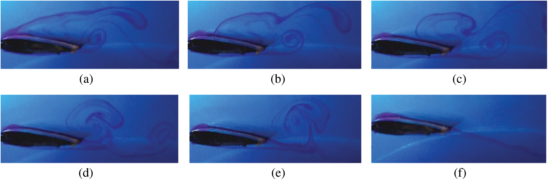
Figure 14: Pulse line evolutions of the hydrofoil under the action of streamwise Lorentz force (experimental results). (a) 1.0 s, (b) 12.0 s, (c) 15.0 s, (d) 19.0 s, (e) 25.0 s and (f) 42.0 s
Fig. 15 displays the vorticity diagram of the flow field around the hydrofoil because of the streamwise Lorentz force (calculated results). In the numerical simulation, the streamwise force is applied at dimensionless computation t = 1.0. From the experiment and numerical simulation diagrams, the flow field structures remain the same without the addition of the force applied onto the hydrofoil, which indicates that this Lorentz distribution model can effectively describe the flow field characteristics around the hydrofoil.
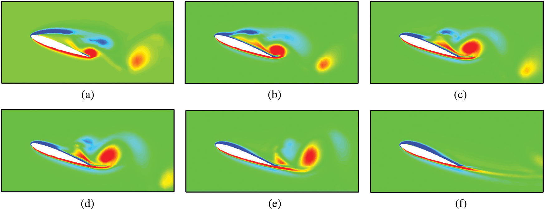
Figure 15: Vorticity evolutions of the flow field around the hydrofoil because of streamwise Lorentz force (calculated results). (a) t = 0.66, (b) t = 1.04, (c) t = 1.08, (d) t = 1.10, (e) t = 1.14 and (f) t = 1.30
This study investigated the field-intensity distribution characteristics surrounding an electromagnetic propulsion unit in seawater (a weak electrically conducting fluid environment). The results indicated the following:
1. The alternatively arranged electric or magnetic poles can produce a Lorentz force with periodic fluctuations in the spanwise direction, and its maximum strength is exhibited right above the edges of the electrode and magnetic poles; however, the average force strength rapidly decays along the wall-normal direction.
2. A simplified mathematical model of the electromagnetic field was developed, and the 3D numerical simulation results were obtained and presented.
3. Based on the simplified Lorentz force distribution function in the source term of the Navier-Stokes equations, numerical simulation was performed for the flow field evolution around a hydrofoil (NACA0012). Meanwhile, a water tunnel experiment was conducted to verify the numerical results and the effectiveness of the Lorentz force action.
4. Therefore, the Lorentz force propulsion method can suppress the magnetic leakage phenomenon and can offer appropriate electromagnetic safety. In this study, some of the variables are non-dimensional and only discuss the general relative distribution or changing trends of flow fields. However, the grid independence test should also be discussed. In further studies, the influence of the current intensity on the electromagnetic environment and quantification of MHD propulsion efficiency should receive significant attention.
Funding Statement: This work was supported by the National Natural Science Foundation of China [Grant No. 11702139].
Conflicts of Interest: The authors declare that they have no conflicts of interest to report regarding the present study.
1. Lecordier, J. C., Browne, L. W. B., Masson, S. L., Dumouchel, F., Paranthoen, P. (2000). Control of vortex shedding by thermal effect at low Reynolds numbers. Experimental Thermal and Fluid Science, 21(4), 227–237. DOI 10.1016/S0894-1777(00)00007-8. [Google Scholar] [CrossRef]
2. Zhang, H., Fan, B., Chen, Z., Zhou, B. (2008). Suppression of flow separation around a circular cylinder by utilizing Lorentz force. China Ocean Engineering, 22, 87–95 (in Chinese). [Google Scholar]
3. Gailitis, A., Lielausis, O. (1961). On a possibility to reduce the hydrodynamical resistance of a plate in an electrolyte. Applied Magnetohydrodynamics, 12, 143–146. [Google Scholar]
4. Liu, H., Zhou, B., Liu, Z., Ji, Y. (2013). Numerical simulation of flow around a body of revolution with an appendage controlled by electromagnetic force. Proceedings of the Institution of Mechanical Engineers Part G Journal of Aerospace Engineering, 227(2), 303–310. DOI 10.1177/0954410011433120. [Google Scholar] [CrossRef]
5. Ji, Y., Zhou, B., Huang, Y. (2018). Mechanism of electromagnetic flow control enhanced by electro-discharge in water. Chinese Physics Letters, 35(5), 055203. DOI 10.1088/0256-307X/35/5/055203. [Google Scholar] [CrossRef]
6. Dousset, V., Potherat, A. (2008). Numerical simulations of a cylinder wake under a strong axial magnetic field. Physics of Fluids, 20(1), 017104. DOI 10.1063/1.2831153. [Google Scholar] [CrossRef]
7. Fan, J., Guo, Q., Liang, Y., Zeng, G., Li, J. et al. (2018). High-temperature superconducting magnetic separation technology in China. Modern Physics Letters B, 32(30), 1830005. DOI 10.1142/S0217984918300053. [Google Scholar] [CrossRef]
8. Fradkin, E., Kivelson, S. A., Tranquada, J. M. (2015). Colloquium: Theory of intertwined orders in high temperature superconductors. Reviews of Modern Physics, 87(2), 457–482. DOI 10.1103/RevModPhys.87.457. [Google Scholar] [CrossRef]
9. Flores-Livas, J. A., Sanna, A., Gross, E. K. U. (2016). High temperature superconductivity in sulfur and selenium hydrides at high pressure. European Physical Journal B, 89(3), 63. DOI 10.1140/epjb/e2016-70020-0. [Google Scholar] [CrossRef]
10. Liu, Z., Gu, J., Zhou, B., Ji, Y., Huang, Y. et al. (2014). Surface propulsion and vector control characteristics of electromagnetic fluid based on hull body. Acta Physica Sinica, 63(7), 1–11 (in Chinese). [Google Scholar]
11. Liu, Z., Zhou, B., Liu, H., Ji, Y., Huang, Y. (2013). Numerical investigation on feedback control of flow around an oscillating hydrofoil by Lorentz force. Fluid Dynamics Research, 45(3), 035502. DOI 10.1088/0169-5983/45/3/035502. [Google Scholar] [CrossRef]
12. Pham, H. Q., Trinh, Q. T., Doan, D. T., Tran, Q. H. (2018). Importance of magnetizing field on magnetic flux leakage signal of defects. IEEE Transactions on Magnetics, 54(6), 1–6. DOI 10.1109/TMAG.2018.2809671. [Google Scholar] [CrossRef]
13. Posdziech, O., Grundmann, R. (2001). Electromagnetic control of seawater flow around circular cylinders. European Journal of Mechanics-B/Fluids, 20(2), 255–274. DOI 10.1016/S0997-7546(00)01111-0. [Google Scholar] [CrossRef]
14. Liu, Z., Zhou, B., Liu, H., Liu, Z., Ji, Y. (2011). Direct force control of a rudder with the action of a coplanar waveguide product microwave. Chinese Physics Letters, 28(9), 094703. DOI 10.1088/0256-307X/28/9/094703. [Google Scholar] [CrossRef]
15. Crawford, C. H., Karniadakis, G. E. (1997). Reynolds stress analysis of EMHD-controlled wall turbulence. Part I. Streamwise forcing. Physics of Fluids, 9(3), 788–806. DOI 10.1063/1.869210. [Google Scholar] [CrossRef]
16. Berger, T. W., Kim, J., Lee, C., Lim, J. (2000). Turbulent boundary layer control utilizing the Lorentz force. Physics of Fluids, 12(3), 631–649. DOI 10.1063/1.870270. [Google Scholar] [CrossRef]
17. Weier, T., Gerbeth, G., Mutschke, G., Lielausis, O., Lammers, G. (2003). Control of flow separation using electro-magnetic forces. Flow, Turbulence and Combustion (Formerly Applied Scientific Research), 71(1–4), 5–17. DOI 10.1023/B:APPL.0000014922.98309.21. [Google Scholar] [CrossRef]
18. Liu, Z., Tang, Z. (2021). Numerical analysis of multi-scale pressure pulsation on the energy accumulation for submarine-based tracking and pointing systems. Measurement and Control, 60(8), 84701–084701. [Google Scholar]
 | This work is licensed under a Creative Commons Attribution 4.0 International License, which permits unrestricted use, distribution, and reproduction in any medium, provided the original work is properly cited. |