Materials Processing
| Fluid Dynamics & Materials Processing |
DOI: 10.32604/fdmp.2021.013535
ARTICLE
Analysis of the Agglomeration of Powder in a Coaxial Powder Feeding Nozzle Used for Laser Energy Deposition
1School of Mechanical Engineering, Liaoning Technical University, Fuxin, 123000, China
2Key Laboratory of Large-Scale Industrial and Mining Equipment of Liaoning Province, Fuxin, 123000, China
*Corresponding Author: Chenguang Guo. Email: gchg_neu@163.com
Received: 10 August 2020; Accepted: 15 January 2021
Abstract: To improve the agglomeration of powder in a coaxial powder feeding nozzle used in the frame of a laser energy deposition technique, the influence of several parameters must be carefully assessed. In the present study the problem is addressed by means of numerical simulations based on a DEM-CFD (Discrete Element Method and Discrete Element Method) coupled model. The influence of the powder flow concentration, powder flow focal length and the amount of powder at the nozzle outlet on the rate of convergence of the powder flow is considered. The role played by the nozzle outlet width, the angle between the inner and outer walls and the powder incident angle in determining the powder flow concentration is also considered. The results show that, with increasing of nozzle outlet width, the powder flow concentration per unit volume at the nozzle focal point undergoes a non-monotonic behaviour (it first increases and then decreases). When the nozzle outlet width δ is 1.00 mm, the powder flow concentration at the focal point is maximal and the powder flow convergence can be considered optimal. By increasing the angle between the inner and outer walls, the powder flow concentration related to the upper focus decreases, the focus diameter increases and the powder flow aggregation worsens. The powder flow concentration increases first and then decreases with increasing incident angle. When the incident angle θ is 30°, the powder flow exhibits the best agglomeration properties. When the outlet width is smaller, the angle between the inner and outer walls is larger, and when the incident angle is set at 30°, the powder flow concentration of the coaxial nozzle can be effectively improved.
Keywords: DEM-CFD coupling; gas-solid two-phase flow; coaxial powder feeding; nozzle structure; powder flow agglomeration
Laser energy deposition is a newly formed technology that has developed rapidly in recent years. Computer-aided design, digital control and laser rapid prototyping are used to enable component forming that can considerably shorten the manufacturing cycle [1–6]. Coaxial powder feeding can realize the coaxial output of the laser and powder, improve the quality of the cladding layer and implement spatial multidimensional cladding. As a key component of the powder transport process, the structure of the coaxial nozzle is an essential influencing factor on powder agglomeration during laser energy deposition [7–9].
Scholars have researched powder transport characteristics and the trends of different nozzle structural parameters. Kovalenko et al. [10] developed an efficient multichannel coaxial powder feeding nozzle so that powder particles with different properties could be transported to the laser processing area at the same time. Based on the CFD method, the powder flow distribution and concentration were analysed and studied, and their research showed that the use of multichannel coaxial powder feeding nozzles could achieve the powder flow distribution and concentration required for production. Pekkarinen et al. [11] studied the relationship between the nozzle powder feeding angle and the carrier gas flow based on the CFD method. Their study showed that as the nozzle powder feeding angle decreased, the powder flow became more stable. Bi et al. [12] developed a compact coaxial powder feeding nozzle with an integrated monitoring system using infrared temperature signal monitoring to ensure product quality after cladding. Research has shown that the nozzle can effectively monitor and control the laser cladding process and obtain real-time acquisition of the working status of the powder nozzle. Liu et al. [13] analysed the powder flow concentration distribution in a coaxial powder feeding nozzle based on the CFD method. Their study showed that due to the collision of particles within the inner wall of the nozzle, the particle diameter and the elastic recovery coefficient of the particles affected the powder flow velocity at the nozzle outlet and the convergence characteristics of the powder flow below the nozzle outlet. Wang et al. [14] developed a four-hole coaxial powder feeding nozzle. Based on the CFD method, they studied the influences of different powder flow channel outlet shapes and different powder flow channel inclination angles on the powder flow field. Their study showed that the powder flow channel outlet was contracted. When the inclination angle of the outlet and the powder flow channel was 70°, the quality of cladding forming was improved. Park et al. [15] established an asymmetric nozzle structure model based on the CFD method and studied a highly convergent particle area. Their study showed that an asymmetric nozzle structure effectively aggregated particles without clogging the nozzle entrance. Liang et al. [16] used numerical simulations and experiments to study the effect of inner cone depth change on jet performance. Their study showed that as the inner cone depth increased, the injection angle became larger, the axial velocity drop rate decreased, and the spray distance increased.
Current research on the influence of the nozzle structure on powder flow agglomeration has mainly focused on air flow field models in CFD [17] to analyse changes in the powder flow field [18] but has ignored the movement trajectory of discrete particles and the interactions between the moving particles and the air flow field. Therefore, the flow field distributions of gas-solid two-phase flows within the nozzle powder cavity may have been inaccurately simulated [19]. In this paper, by considering collisions among particles and between particles and the inner wall of the nozzle, a DEM-CFD bidirectional coupling model [20–26] is adopted to establish an Euler model for gas-solid two-phase flow [27,28]. The powder flow concentration, powder flow focal length and amount of powder at the nozzle outlet are used as factors to measure powder flow agglomeration. The change rules of nozzle structural parameters, such as the nozzle outlet width, the angle between the inner and outer walls and the powder incident angle, on powder flow agglomeration are analysed.
In the calculation process of a coupled model of gas-solid two-phase flow based on a Euler model, the conservation equation of particles is calculated by the DEM model. The DEM model transfers the volume fraction, position and velocity of the particles to the CFD model. The CFD model introduces the force of the fluid on the particles into the coupled solver. The CFD model combines the data transmitted by the DEM model to calculate the force acting on the particle surface and transfers it to the DEM model. The DEM model analyses the position and velocity information of the particles under the force in the new calculation step and passes the information to CFD for the next iteration. The process is repeated until the simulation analysis converges.
To simulate the particle flow state effectively, the equivalent diameter of an equal volume sphere is adopted to describe the powder particles [29], as shown in Eq. (1):
where dev is the equivalent diameter of a ball of equal volume and V is the volume of the particle. A soft sphere model is used to describe the particles, which allows for a small amount of overlap during a collision between particles. The force created when the particles are in contact is shown in Fig. 1. When particles i and j are in collision and contact, there is a normal overlap amount that is designated as α. Fdt,ij is the tangential contact force of particle i acting on particle j; Fct,ij is the tangential contact force of particle j acting on particle i; Fdn,ij is the normal contact force of particle i acting on particle j; Fcn,ij is the normal contact force of particle j on particle i; ωi and ωj are the angular velocities of particle i and particle j; vi and vj are the velocities of particle i and particle j; and gi and gj are the gravitational acceleration of particle i and particle j, respectively. The contact force between particles is simplified as damper βn, spring kn, and slider μ. A simplified model of the particle contact forces is shown in Fig. 2.
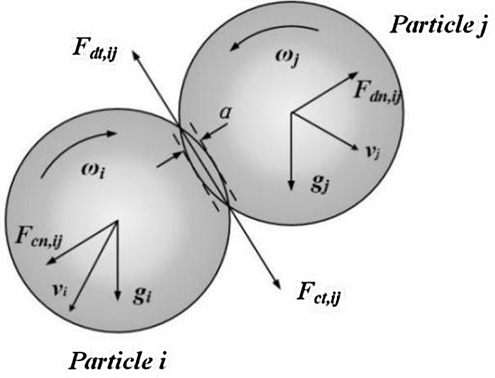
Figure 1: Simplified model of contact forces between particles
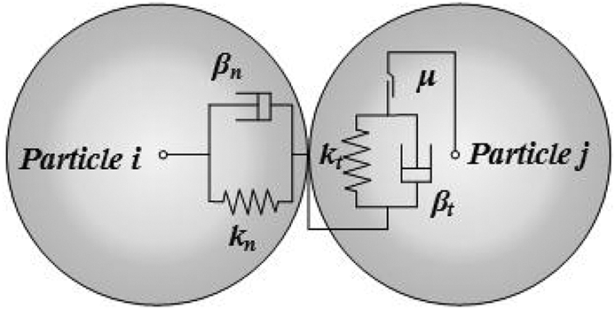
Figure 2: Simplified model of contact forces between particles
When two spherical particles make contact and collide in space with radii R1 and R2, respectively, the normal contact force Fn can be expressed as Eq. (2):
where E' is the equivalent elastic modulus; R' is the equivalent particle radius; and ε is the normal overlap amount during collision. The formulas for solving the three parameters E', R' and ε are shown in Eqs. (3)–(5):
The tangential contact force Ft can be obtained as follows:
where εt is the tangential overlap amount when the particles collide and St is the tangential contact stiffness, which is shown in Eq. (7):
where G' is the equivalent shear modulus.
The tangential damping force Ft between two particles is shown in Eq. (8):
where β is the coefficient; m* is the equivalent mass of the particle; and vtrel is the relative tangential velocity when the particle collides. β and m* can be obtained by Eqs. (9) and (10):
The basic governing equations of the gas phase include the mass, momentum and energy conservation equations [30,31]. The powdering airflow and shielding gas are incompressible, stable and turbulent [32–35]. The heat transfer during powder transport is not considered in this study. Navier-Stokes governing equations are used in the DEM-CFD model. The balance equations for mass and momentum for the solid-gas flow are shown in Eqs. (11) and (12).
where ρ is the density of the gas; t is time; u is the velocity of the gas; ε is the volume fraction of the gas.
where p is the pressure of the gas; μ is the gas viscosity; FD is the interaction between the gas and the particles; and V is the volume of a CFD grid cell.
The turbulent energy equation can be represented as Eq. (13):
The turbulent dissipation rate equation can be written as follows:
where k is the turbulent flow energy; e is the turbulent dissipation rate; i, j = 1, 2, 3; and μ = μ0 + μt (μ0 is the molecular viscosity; μt is the turbulent viscosity). Gk represents the turbulent kinetic energy generated by the average velocity gradient; Gb represents the turbulent kinetic energy generated by buoyancy; Pt is the turbulent Prandtl number, and the correction coefficient can be obtained according to the standard k-ε turbulence model. σk = 1.0, σs = 1.0, C1 = 1.0, and C2 = 1.0.
3 Simulation Model Construction
The calculation domain of the coaxial nozzle simulation model is mainly divided into three parts. The upper part is a circular powder channel, the middle part is a funnel-shaped channel with different inclination angles, and the lower part is a cylindrical calculation domain of powder distribution. As shown in Fig. 3, the powder is injected from the four inlets, which are evenly distributed above the nozzle, gathered after passing through the funnel-shaped channel, and then ejected from the outlet into the cylindrical calculation domain.
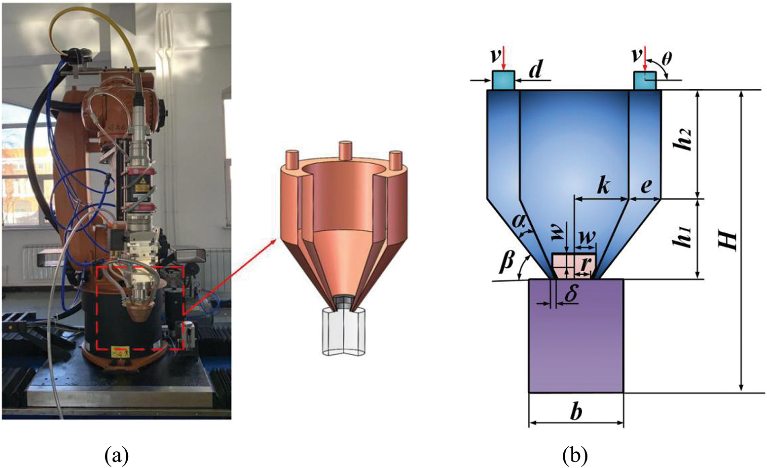
Figure 3: Coaxial powder feed nozzle. (a) Three-dimensional structural model. (b) Two-dimensional plane model
To describe the geometric characteristics of the calculation domain of the coaxial powder feeding nozzle, the main parameters are set as shown in Tab. 1, where d is the diameter of the powder flow inlet; h1 and h2 are the heights of the funnel-shaped tapered ring and annular powder flow channels, respectively; α is the angle between the inner and outer walls of the funnel-shaped tapered ring channel; β is the angle between the outer wall of the type channel; δ is the nozzle outlet width; m is the height of the central light path protective gas ring channel; w and r are the central light path protective gas inlet and outlet radius, respectively; b is the length of the cylindrical calculation area; H is the total height of the nozzle and the calculation domain; and θ is the incident angle of powder flow.
Table 1: Initial values of characteristic parameters of the calculation domain

ICEM grid preprocessing software is adopted to mesh the nozzle and the calculation domain. A hexahedral structured grid is selected to improve the quality and efficiency of the computing grid. Due to the different powder concentrations caused by different nozzle locations and the calculation domain, the key component grid should be refined, and the remaining grid should be appropriately divided into sparse structure grids on the premise of meeting the calculation requirements. The mesh sizes of the nozzle inlet, the cylindrical domain and the nozzle ring channel calculation domain are set as 0.8 mm, 0.75 mm and 1.5 mm, respectively. Since the contact parts of the three calculation domains are at the computing centre, the grid size is set to be 0.2 mm, and the partitioned grid is optimized. The mesh quality of the grids is set to 0.4 or above. The aspect ratio is set within 0–1, and the Jacobi matrix is set to 0.7 or above. The divided grid is shown in Fig. 4, and the total number of grids is 377959. By using FLUENT to solve the CFD model, the grid is checked after importing the grid file generated by ICEM into FLUENT. After determining that there is no negative number in the minimum volume grid, the correct unit is selected, and the grid is reordered to decrease the matrix bandwidth and improve the calculation efficiency.
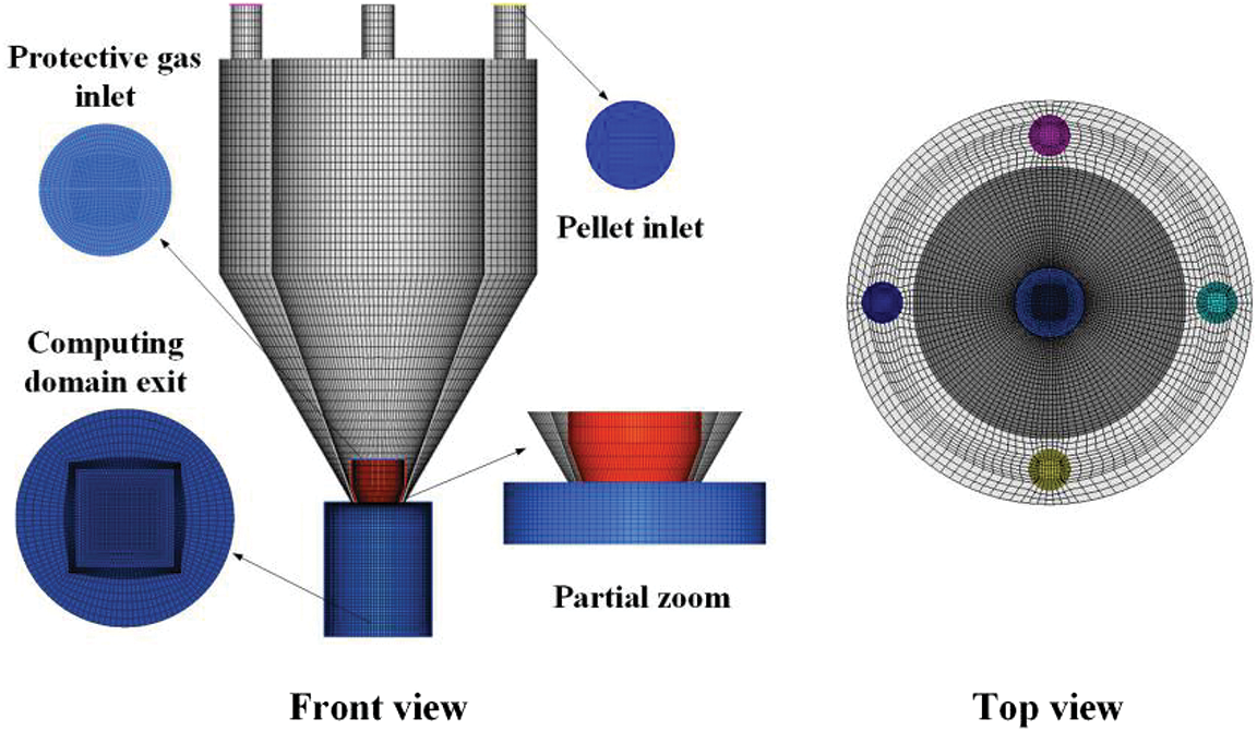
Figure 4: Structured grids for coaxial feeding nozzle
The residual value of the FLUENT model is set as 0.001. The residual error is set to ensure that the relative difference of all equations in the adjacent time steps is within the specified range and to maintain the continuity of the gas-solid two-phase calculation. The simulation includes the continuity equation, momentum equation, k turbulent kinetic energy equation, e turbulent energy dissipation rate equation and particle phase equation. The simulation adopts a pressure-based analysis model, and absolute velocity is adopted. Since the analysis model involves the coupling of multiphase flow, the simulation process is an unsteady process, which needs to be solved transiently. The direction of gravity set in the FLUENT model is the same as that in the EDEM model. The powdering airflow and shielding gas are incompressible, stable and turbulent. The standard k-e model is selected for the turbulent viscosity model. The multiphase flow model is the Euler model, and the number of phases is set to 2. The main phase is N2, and the second phase is the particles. The inlets of powder flow and protective gas are set to velocity inlets, and the speed direction is perpendicular to the boundary. The velocities of carrier powder gas v and shielding gas v1 are 4 m/s and 1.5 m/s, respectively. The nozzle wall is set as the wall, and the nozzle outlet is the pressure outlet. Since the nozzle boundary is a free outlet, the pressure is set to 0 Pa. The exit boundary diameter of the calculation domain is 20 mm. The backflow turbulence intensity should not be set too large, so the backflow intensity in this manuscript is set to 0.5%. A phase-coupled SIMPLE algorithm is used. Spatial discretization is used in the discretization scheme. To ensure the convergence of the coupled model, a second-order upwind is selected.
Since the time step has a greater impact on the convergence of the DEM model than on the CFD model, the DEM time step is first determined in the coupled DEM-CFD model. The time step of the CFD model is an integer multiple of the time step of the DEM model. The calculation of the velocity and position information of the particles in the DEM model is a transient process. In the DEM model, it is assumed that the motion attributes of particles within a time step are unchanged. To improve the accuracy of the DEM model, the percentage of the Rayleigh time step is used to determine the time step of the model. The Rayleigh time step is the time required for the polarized wave generated by particle contact to pass through the hemisphere, which is shown in Eq. (17):
where G is the shear modulus of the particle and ρ is the density of the particle. In the case of satisfying numerical convergence, the time step of the model is generally 5–40% of the Rayleigh time step. The time step of the DEM model in this manuscript is set to 20% of the Rayleigh time step. The time step in the CFD model is set to 80 times the time step of the DEM model, and the value is 8e-5 s.
3.2 DEM-CFD Simulation Analysis Model Verification
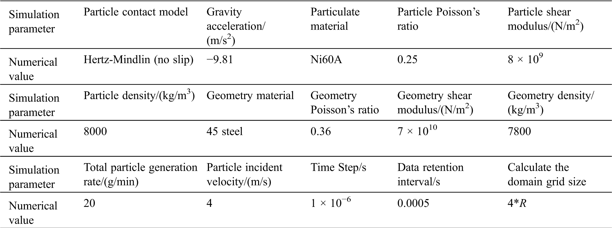
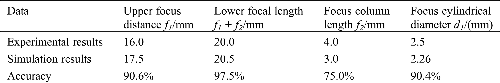
To verify the rationality and reliability of the model, a powder transport verification experiment is performed. The powder feeding rate vf is 20 g/min. In the simulation, the particle size is set as 30 μm, and the specific parameters are shown in Tab. 2. Fig. 5a shows a characteristic diagram of the powder flow distribution. In the figure, f1 is the distance between the upper focal point of the powder flow and the nozzle outlet, which is the upper focal length; f2 is the distance between the upper and lower focal points of the powder flow, which is the focal length; f1 + f2 is the lower focal length; f3 is the laser defocusing amount; d1 and d2 are the diameter of the powder focal column and the spot diameter; and δ is the nozzle outlet width. Fig. 5b shows the powder flow velocity trace of the powder nozzle, and Fig. 5c shows the DEM-CFD coupling simulation velocity trace.
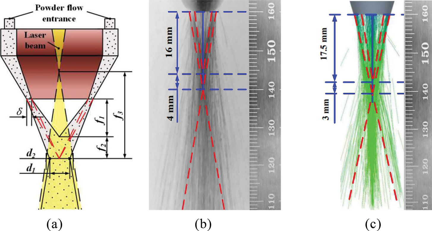
Figure 5: Comparison chart of experimental and simulation results. (a) Distribution characteristics of powder flow. (b) Coaxial powder feed nozzle powder flow velocity trace. (c) DEM-CFD coupling simulation speed trace
Table 2: EDEM simulation parameter settings
The comparison between the simulated and experimental results is shown in Tab. 3. The accuracy of the upper focal length, lower focal length and focal diameter of the powder flow reached more than 90%, and the accuracy of the focal length was 75%. The simulated and experimental results have the same morphology of the powder flow, and the convergence position and concentration distribution are consistent. The DEM-CFD bidirectional coupling model has a high level of accuracy and is suitable for analysing the trends of the nozzle structural parameters on powder flow agglomeration.
Table 3: Comparison of experimental and simulation results
3.3 Simulation Analysis Experiment Scheme
The nozzle structure directly affects the trajectory of the powder flow and the agglomeration after being sprayed out. Based on the single factor method, the influences of the nozzle outlet width δ, the angle between the inner and outer walls α and the powder incident angle θ on the powder flow agglomeration are analysed. The velocities of the carrier powder gas and shielding gas are v = 4 m/s and v1 = 1.5 m/s, respectively. The powder feeding rate vf is 20 g/min. The angle between the nozzle wall and the horizontal plane is β = 60°. The experimental scheme is shown in Tab. 4.
Table 4: Experimental protocol parameters
4 Result Verification and Analysis
4.1 Measurement Index of Powder Agglomeration
To quantify the agglomeration of powder flow, the powder flow concentration per unit volume MP, as shown in Eq. (18), is introduced as a measurement index, which is the proportion of powder particles in a unit volume.
where VP is the volume occupied by powder particles per unit volume and Vf is the volume occupied by air per unit volume. The greater the value of MP per unit volume of powder flow is, the better the powder flow agglomeration.
4.2 Influence of Nozzle Outlet Width δ
The angle between the inner and outer walls of nozzle α is 10°. θ is set to 90°. β is set to 60°. With δ set to 0.6 mm, 1.0 mm, 1.1 mm, and 1.2 mm, numerical simulation analyses and experimental verifications are carried out.
Fig. 6 shows a comparison of the simulation results and experimental results for nozzles with different δ values. As shown in Fig. 6, the simulation results and the experimental results are basically the same. The concentration position of the powder flow basically corresponds to the general trend of the concentration distribution. As shown in Tab. 5, the accuracy of the upper and lower focal lengths of the powder flow reaches more than 95%, indicating that this simulation model possesses good applicability. As shown in Fig. 6 and Tab. 5, the simulation results are slightly different from the experimental results. The main reason is that the powder particles used in the experiment have nonspherical bodies, and the powder particles are assumed to be spherical in the simulation analysis. The properties of the simulated individual particles may be different from the actual ones, resulting in larger deviations in their flight trajectories.
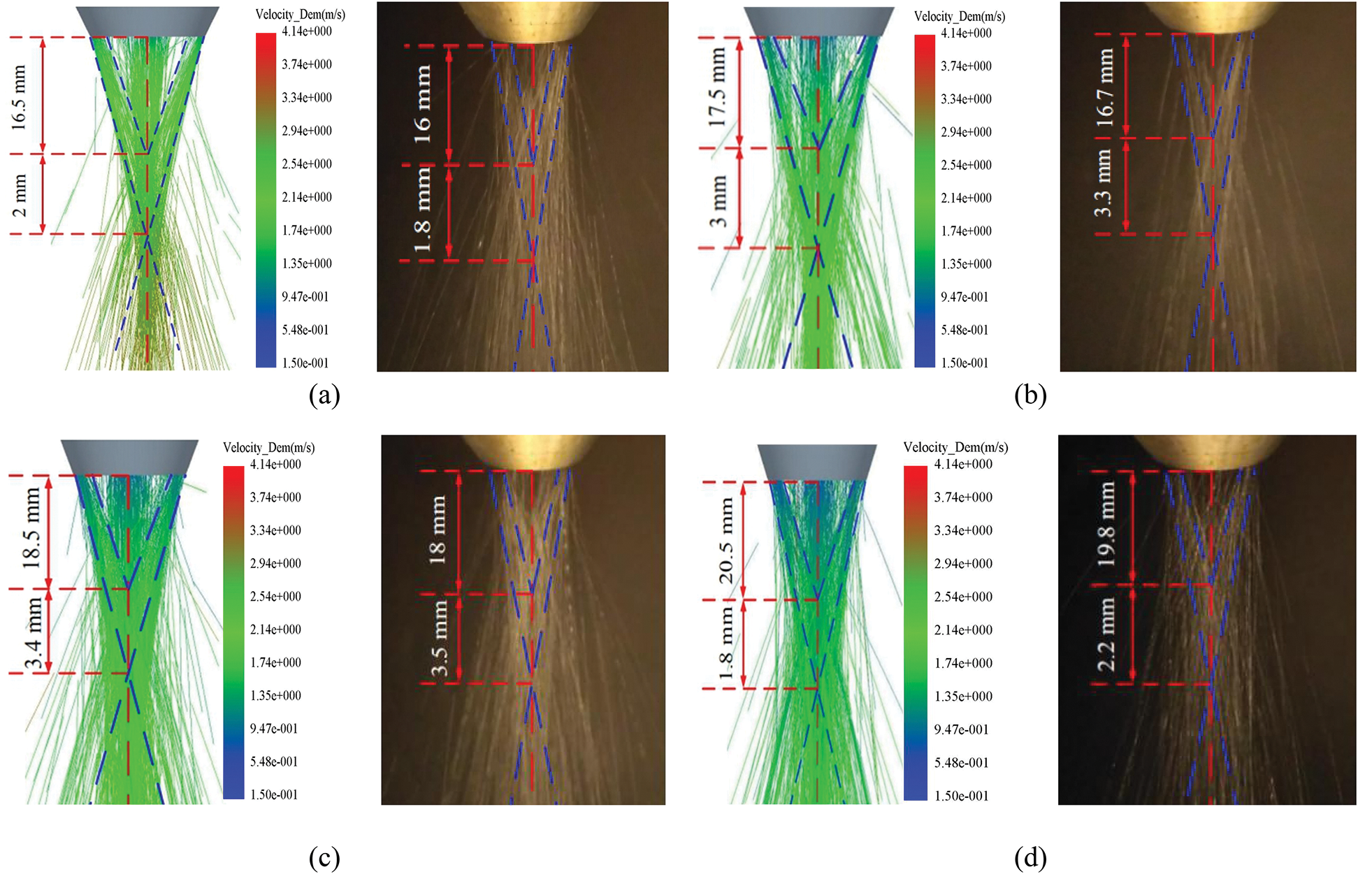
Figure 6: Comparison of simulation results and experimental results for nozzles with different δ values. (a) δ = 0.6 mm. (b) δ = 1.0 mm. (c) δ = 1.1 mm. (d) δ = 1.2 mm
Table 5: Comparison of simulation and experimental data
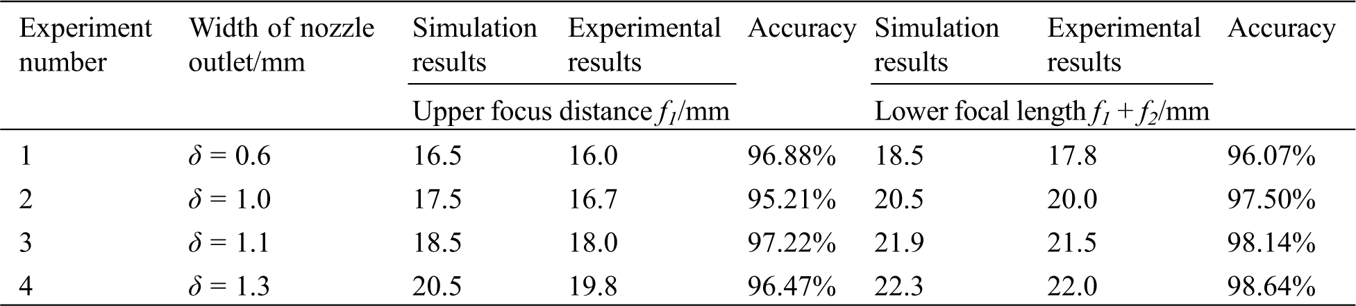
Fig. 7 shows the axial powder flow concentration distribution per unit volume for nozzles with different δ values. As shown in Fig. 7, when δ is 0.6 mm, the upper focal point of the powder flow is at Y = 16.5 mm, which is the closest to the nozzle outlet. The unit volume powder concentration is 0.0086. The lower focal point is at Y = 18.5 mm, and the unit volume density of powder flow is 0.0065. As δ becomes smaller, the powder jet ejection speed becomes larger, the powder flow aggregation is improved, and the powder flow focus position moves up. When δ is 1.00 mm, the powder flow concentration is at its highest level. The upper focus of the flow moves down to Y = 17.5 mm, and the powder flow concentration per unit volume is 0.0121. When the lower focus moves down to Y = 20.5 mm, the powder flow concentration per unit volume is 0.0078. As δ increases, the concentration of powder flow decreases rapidly, and the focus quickly moves down. When δ is 1.30 mm, the focus on the powder flow is at Y = 20.5 mm, and the distance from the nozzle outlet is the farthest. The powder flow concentration per unit volume is 0.0084.
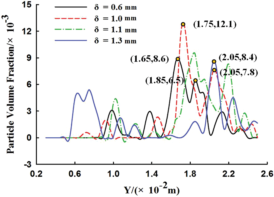
Figure 7: Axial distribution of powder flow concentration per unit volume with nozzle outlet width
Fig. 8 shows the powder flow concentration distribution per unit volume for nozzles with different δ values. As shown in Fig. 8, as δ increases, the powder flow concentration per unit volume shows a trend of first increasing and then decreasing. When δ is 1.00 mm, the powder flow concentration per unit volume at the focal point is maximal, and the powder flow convergence is optimal. As δ increases, the nozzle outlet airflow velocity decreases, the columnar airflow area increases, and the spatial distribution width increases after the powder flow is concentrated. When δ is 1.30 mm, the powder flow concentration per unit volume at the focal point is at its lowest level. This is because an excessively large δ will reduce the jetting speed of the powder flow and worsen powder agglomeration. The focus of powder flow moves down as δ increases. When the powder flow is affected by gravity and air resistance, the ejection speed decreases. The concentration distribution diameter of the powder flow focus becomes larger. The divergence of the powder flow causes the density of the powder flow per unit volume to decrease at the focal point.
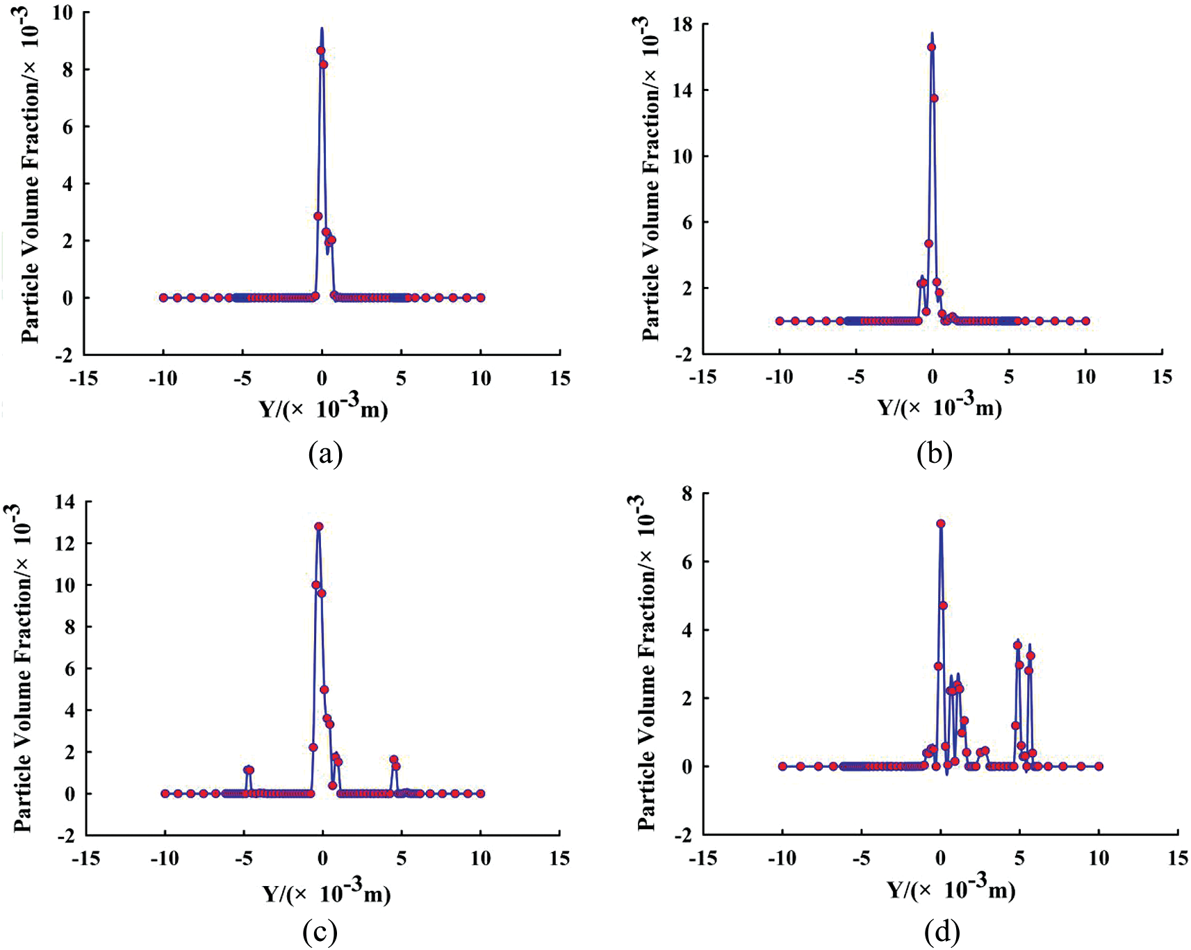
Figure 8: Concentration distribution of powder flow per unit volume for nozzles with different nozzle outlet widths. (a) δ = 0.6 mm. (b) δ = 1.0 mm. (c) δ = 1.1 mm. (d) δ = 1.2 mm
From the above simulation results, it can be seen that δ is an important factor. A small δ value can reduce the powder flow concentration distribution diameter and improve powder flow agglomeration. As shown in Fig. 9, a δ value that is too small will cause a large amount of powder particles to accumulate at the nozzle outlet, thereby hindering the movement of the powder flow and causing the focus concentration of the powder flow to decrease. As δ increases, the focal point of the powder flow collection moves down. The diameter of the powder flow concentration distribution becomes larger. The powder flow concentration per unit volume decreases. The powder flow accumulation becomes worse.
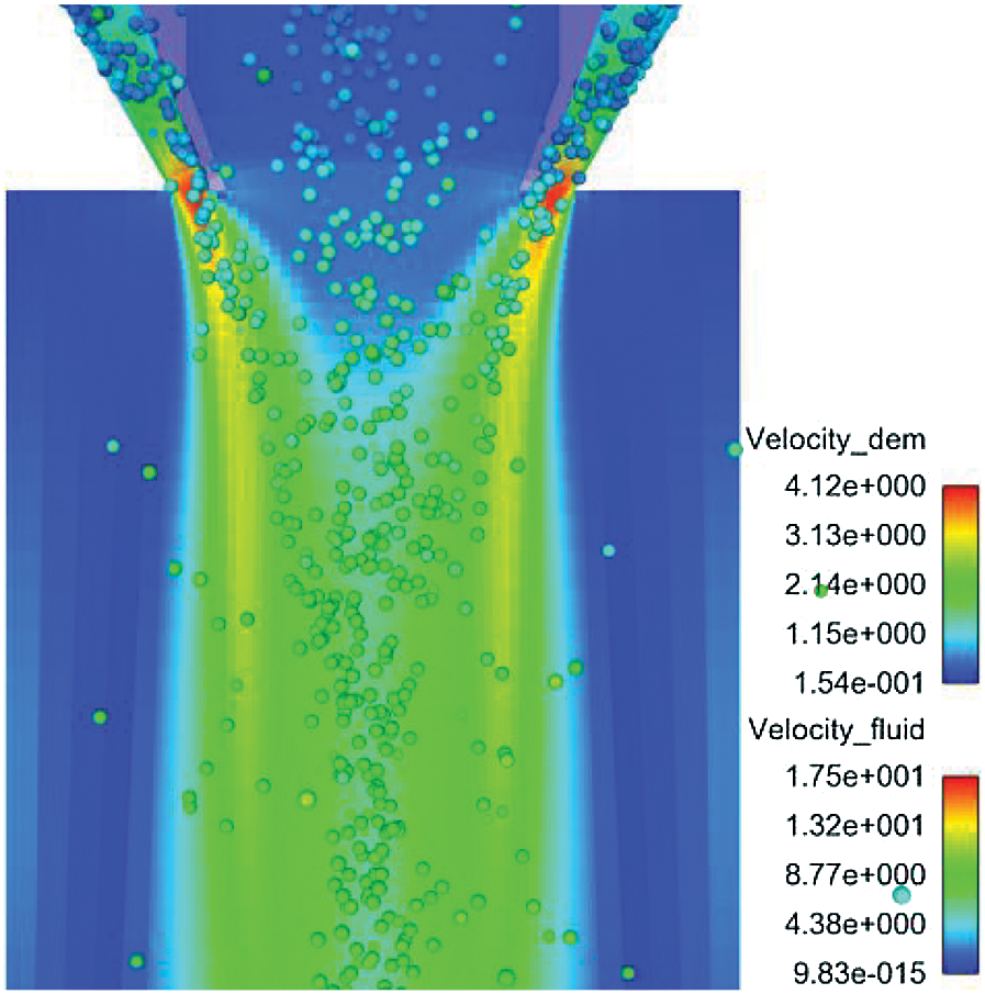
Figure 9: Partial enlarged view of cloud diagram of gas and powder velocity at the small nozzle outlet
4.3 Influence of the Angle between the Inner and Outer Walls of the Nozzle α
θ is set to 90°, δ is set to 1 mm and β is set to 60°. With α set to 8°, 10°, 11°, and 12°, DEM-CFD numerical simulation analyses and experimental verifications are carried out.
Fig. 10 shows a comparison diagram of the simulation results and experimental results for different α values. As shown in Fig. 10, the simulation results and the experimental results are basically the same, and the concentration position of the powder flow basically corresponds to the general trend of the concentration distribution. As shown in Tab. 6, the accuracy of the upper and lower focal lengths of the powder flow reaches more than 95%, indicating that this simulation model possesses good applicability. As shown in Fig. 10 and Tab. 6, the simulation results are slightly different from the experimental results. The main reason is that the powder particles used in the experiment have nonspherical bodies, and the powder particles are assumed to be spherical in the simulation analysis. The properties of the simulated individual particles may be different from the actual ones, resulting in larger deviations in their flight trajectories.
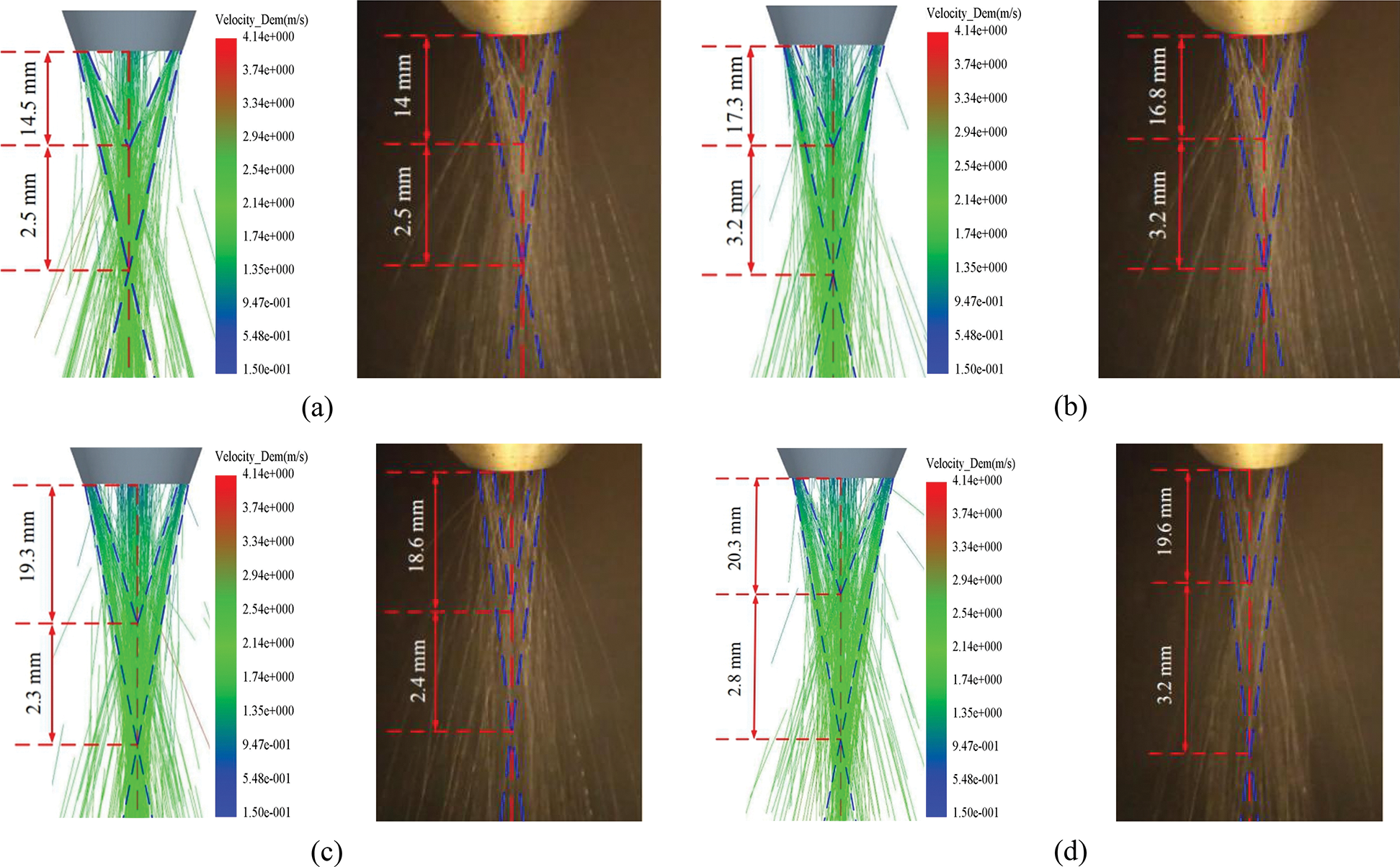
Figure 10: Comparison of simulation results and experimental results for nozzles with different angles between inner and outer walls. (a) α = 8°. (b) α = 10°. (c) α = 11°. (d) α = 12°
Table 6: Comparison of simulation and experimental data
Fig. 11 shows the axial unit volume powder flow concentration distribution for nozzles with different α values. As shown in Fig. 11, when α is 8°, the powder flow concentration per unit volume at the focal point is at its highest level. The upper focus of the powder flow is at Y = 14.5 mm and is closest to the nozzle outlet. The highest concentration of the powder flow per unit volume is 0.0155. The lower focus is at Y = 17 mm, and the concentration of powder flow per unit volume is 0.0105. When α is 12°, the concentration of powder flow per unit volume at the focal point is at its lowest level. The upper focal point of the powder flow is the farthest from the nozzle outlet at Y = 20.3 mm, and the minimum concentration of powder flow per unit volume is 0.0077. The lower focal point is at Y = 23.3 mm, and the powder flow concentration per unit volume is 0.0055. This is because as α decreases, when the powder flow enters the funnel-shaped tapered annular channel of the nozzle, the smaller internal cavity becomes more restrictive to the movement of the powder flow. The number of collisions between powder particles and the inner wall of the nozzle is reduced, and the speed direction of the powder flow is gradually made consistent during the downward movement. The concentration at the focal point gradually increases, and the distance between the focal point and the nozzle outlet gradually decreases. In contrast, as α increases, the rebound angle of the powder particles colliding with the inner wall of the nozzle increases. As the number of collisions between the powder particles and the inner wall of the nozzle increases, the energy loss becomes greater, resulting in a decrease in the velocity of the powder jet when it is ejected and a decrease in the concentration of the focus.
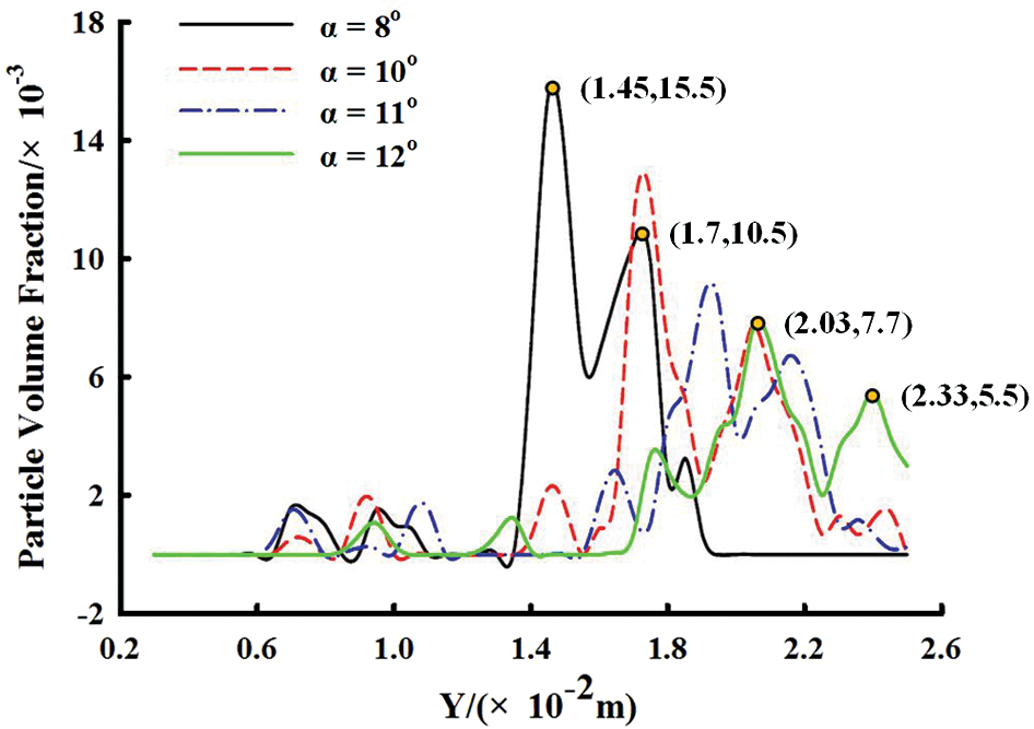
Figure 11: Axial unit volume powder flow concentration distribution for nozzles with different angles between inner and outer walls
Fig. 12 shows the concentration distribution of powder flow per unit volume at different α values. The diameter d1 of the powder coke column of the four nozzles with different α values is 1.94 mm, 2.26 mm, 2.64 mm, and 3.12 mm. It can be seen in the figure that as α increases, d1 becomes larger and the powder flow concentration per unit volume decreases. This is because the larger α values are less restrictive to the space movement of the powder flow, and the number of collisions between the powder particles and the wall surface increases during the downward movement of the powder particles. The energy loss of the powder particles becomes larger, which increases the powder flow concentration distribution diameter and decreases the flow concentration.
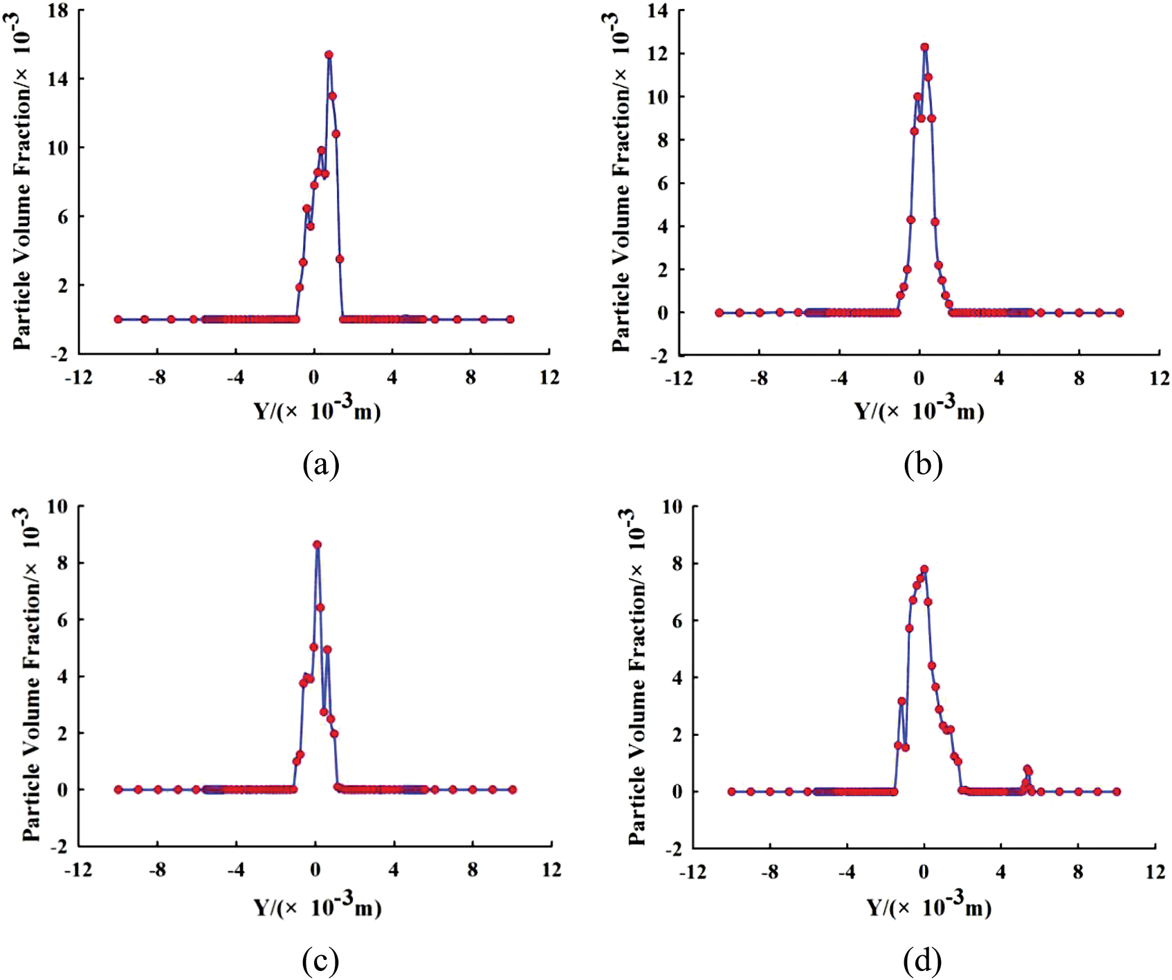
Figure 12: Concentration distribution of powder flow per unit volume at different angles between inner and outer walls. (a) α = 8°. (b) α = 10°. (c) α = 11°. (d) α = 12°
It can be seen from the above simulation results that α has a great influence on powder flow accumulation. As α increases, the powder flow concentration per unit volume decreases. The focal length becomes larger. The powder flow concentration distribution diameter becomes larger. The powder flow divergence angle becomes larger, and the powder flow aggregation becomes worse. Therefore, α should be considered when designing the coaxial powder feeding nozzle. A smaller α value will increase the powder flow concentration per unit volume and reduce the focal distribution diameter of the powder flow concentration. The powder flow divergence angle decreases, which improves the powder utilization rate. A larger α value will increase the divergence angle of powder flow and increase the divergence of powder flow. The larger diameter of the focal column causes the laser spot diameter to be smaller than the powder flow concentration distribution diameter, and the powder utilization rate also appears to decrease.
4.4 Influence of Incident Angle θ on Powder Flow
δ is set to 1 mm. α is set to 10°. β is set to 60°. With θ set to 0°, 30°, 60°, and 90°, numerical simulation analyses and experimental verifications are carried out.
Fig. 13 shows comparisons of the simulation results and experimental results at different θ values of powder flow. As shown in Fig. 13, the simulation results and the experimental results are basically the same, and the concentration position of the powder flow basically corresponds to the general trend of the concentration distribution. As shown in Tab. 7, the accuracy of the upper and lower focal lengths of the powder flow reaches more than 95%, indicating that the simulation model possesses good applicability. As shown in Fig. 13 and Tab. 7, the simulation results are slightly different from the experimental results. The main reason is that the powder particles used in the experiment have nonspherical bodies, and the powder particles are assumed to be spherical in the simulation analysis. The properties of the simulated individual particles may be different from the actual ones, resulting in larger deviations in their flight trajectories.
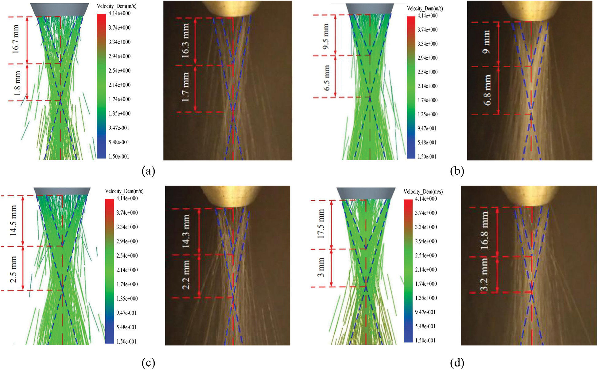
Figure 13: Comparison of simulation results and experimental results for nozzles with different powder incidence angles. (a) θ = 0°. (b) θ = 30°. (c) θ = 60°. (d) θ = 90°
Table 7: Comparison of simulation and experimental data
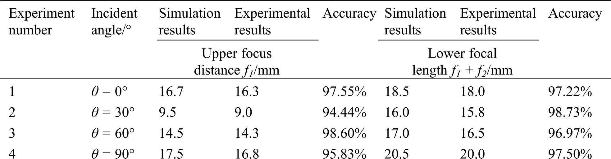
Fig. 14 shows the powder flow concentration distribution per unit volume along the nozzle axis. As shown in Fig. 14a, when θ is 0°, the direction of the powder flow velocity is perpendicular to the cavity of the coaxial powder feeding nozzle, so the powder flow collides strongly with the wall surface, which results in a loss of powder flow energy, a reduction in powder flow speed and a downward shift in powder flow concentration. The upper focus is at Y = 16 mm, and the powder flow concentration per unit volume is 0.0074. The lower focus is at Y = 18.5 mm, and the powder flow concentration per unit volume is 0.01. The powder flow concentration per unit volume of the upper focus is 0.0074. This is lower than the powder flow concentration per unit volume of the lower focus. As shown in Fig. 14b, when θ is 30°, the upper focus is at Y = 9.5 mm, and the powder flow concentration per unit volume is 0.0111. The lower focus is at Y = 16 mm, and the density of powder flow per unit volume is 0.0116. The focus point of powder flow moves upward, and the density of powder flow per unit volume increases at the upper and lower focus points of the powder flow. As shown in Fig. 14c, when θ is 60°, the upper focus of powder flow is at Y = 14.5 mm, and the density of powder flow per unit volume is 0.0086. The lower focus is at Y = 17 mm, and the density of powder flow per unit volume is 0.0048. The powder flow focus moves down, and the powder flow concentration per unit volume of the upper focus is greater than the powder flow concentration per unit volume of the lower focus. As shown in Fig. 14d, when θ is 90°, the upper focus of the powder flow is at Y = 17.5 mm, and the powder flow concentration per unit volume is 0.0121. The lower focus is at Y = 20.5 mm, and the powder flow concentration per unit volume is 0.0078. The powder flow focus moves down, and the powder flow concentration per unit volume increases.
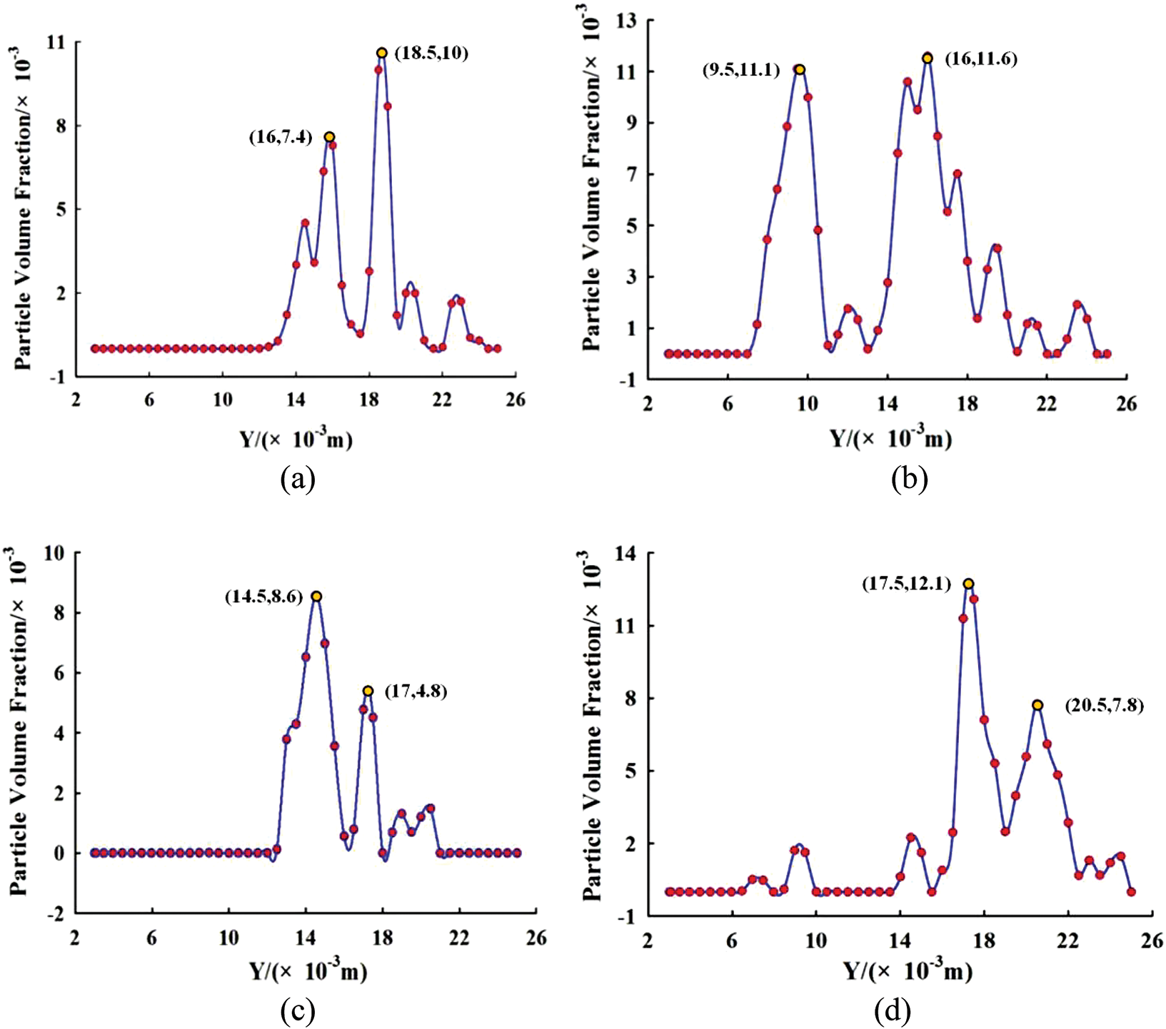
Figure 14: Distribution of powder flow concentration per unit volume in axial direction for nozzles at different injection angles. (a) θ = 0°. (b) θ = 30°. (c) θ = 60°. (d) θ = 90°
Fig. 15 shows the powder particles inside the coaxial powder feeding nozzle under different θ values. As shown in Fig. 15a, when θ is 0°, the powder flow will strongly collide with the inner wall of the nozzle. The powder particles are scattered throughout the cavity of the coaxial powder feeding nozzle. This strong impact makes some particles flow back into the powder flow. The inlet causes the mass flow rate of the powder flow to become unstable. As shown in Fig. 15b, when θ is 30°, the powder flow collides with the inner wall of the nozzle multiple times after the incident and is collected from the nozzle outlet through the funnel-shaped inner wall. As shown in Fig. 15c, when θ is 60°, some particles will aggregate at the beginning of the funnel-shaped inner wall, and some powder particles will return upwards. As shown in Fig. 15d, when θ is 90°, the powder flow enters the nozzle funnel vertically after the incident and is ejected after multiple collisions with the wall, which has fewer collisions than other powder flow incident angles. The spatial distribution of powder is relatively concentrated, and the degree of dispersion of powder particles is small.
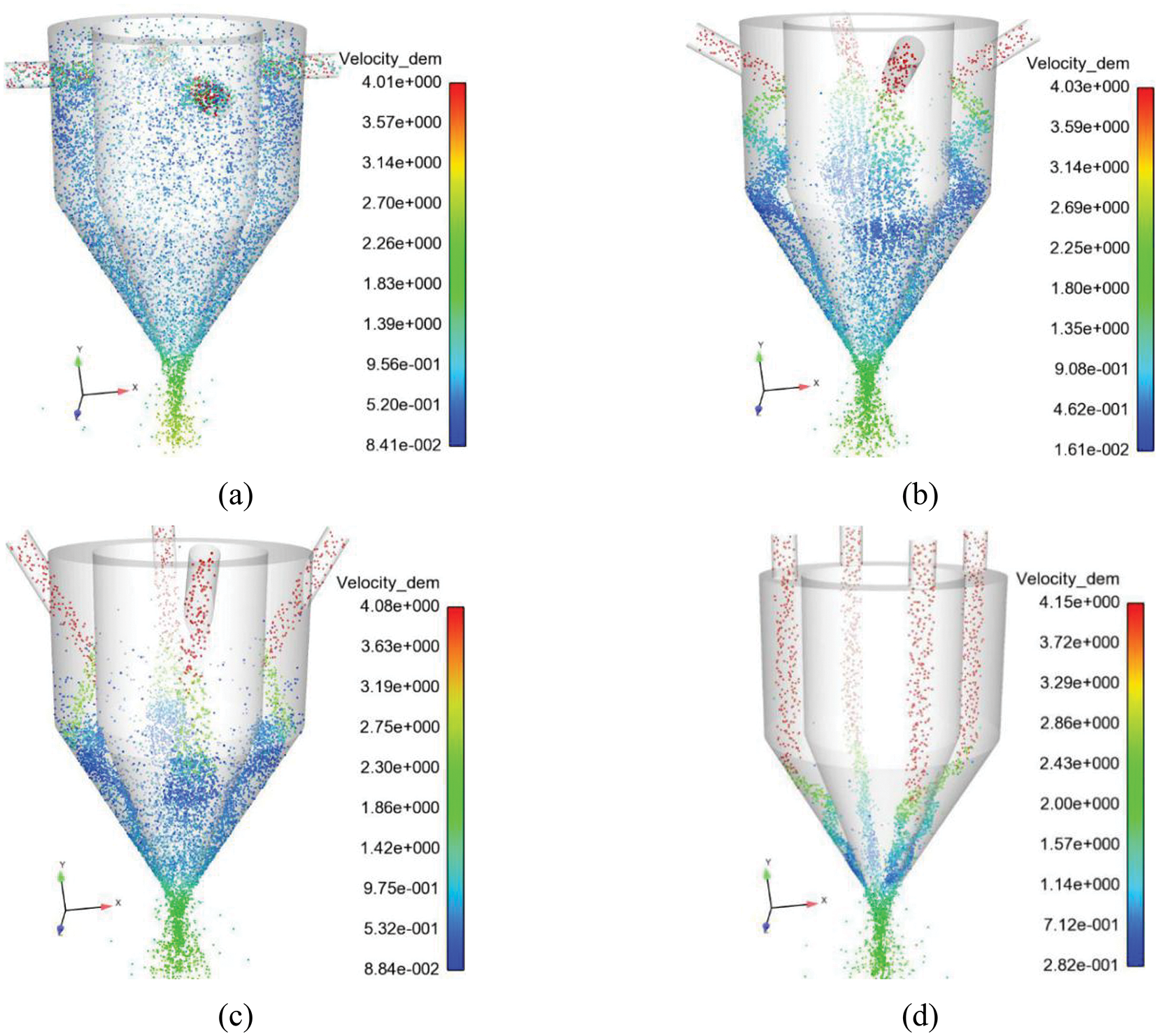
Figure 15: Distribution of powder particles inside the coaxial feed nozzle at different powder injection angles. (a) θ = 0°. (b) θ = 30°. (c) θ = 60°. (d) θ = 90°
Fig. 16 shows the density distribution of powder flow per unit volume at different θ values. It can be seen in the figure that as θ increases, the concentration of the powder flow per unit volume at the focal point shows a trend of first increasing and then decreasing. When θ is 30°, the powder flow concentration per unit volume reaches the maximum, and the powder flow has the best agglomeration. Fig. 17 shows the mass flow rate of the nozzle outlet powder at different θ values. As shown in Fig. 17a, when θ is 0°, the mass flow rate of the powder flow at the nozzle outlet reaches equilibrium at 0.21 s, and the mass flow rate after reaching equilibrium is 14 g/min, which is much smaller than the actual powder feeding rate of 20 g/min. As shown in Fig. 17b, when θ is 30°, the mass flow rate of the nozzle outlet powder reaches equilibrium at 0.15 s, and the mass flow rate after equilibrium is 19 g/min, which is less than the actual powder feeding rate of 20 g/min. This is because the powder rebounds partly during collision with the inner wall of the nozzle, resulting in a mass flow rate slightly lower than the powder feeding rate. As shown in Fig. 17c, when θ is 60°, the mass flow rate of the powder flow at the nozzle outlet reaches equilibrium at 0.15 s, and the mass flow rate after balance is 19.5 g/min. Compared with when θ is 30°, the mass flow rate shows an upward trend. As shown in Fig. 17d, when θ is 90°, the mass flow rate of the powder flow at the nozzle outlet reaches equilibrium at 0.06 s, and the mass flow rate after equilibrium is 20 g/min, which is basically the same as the actual powder feeding rate.
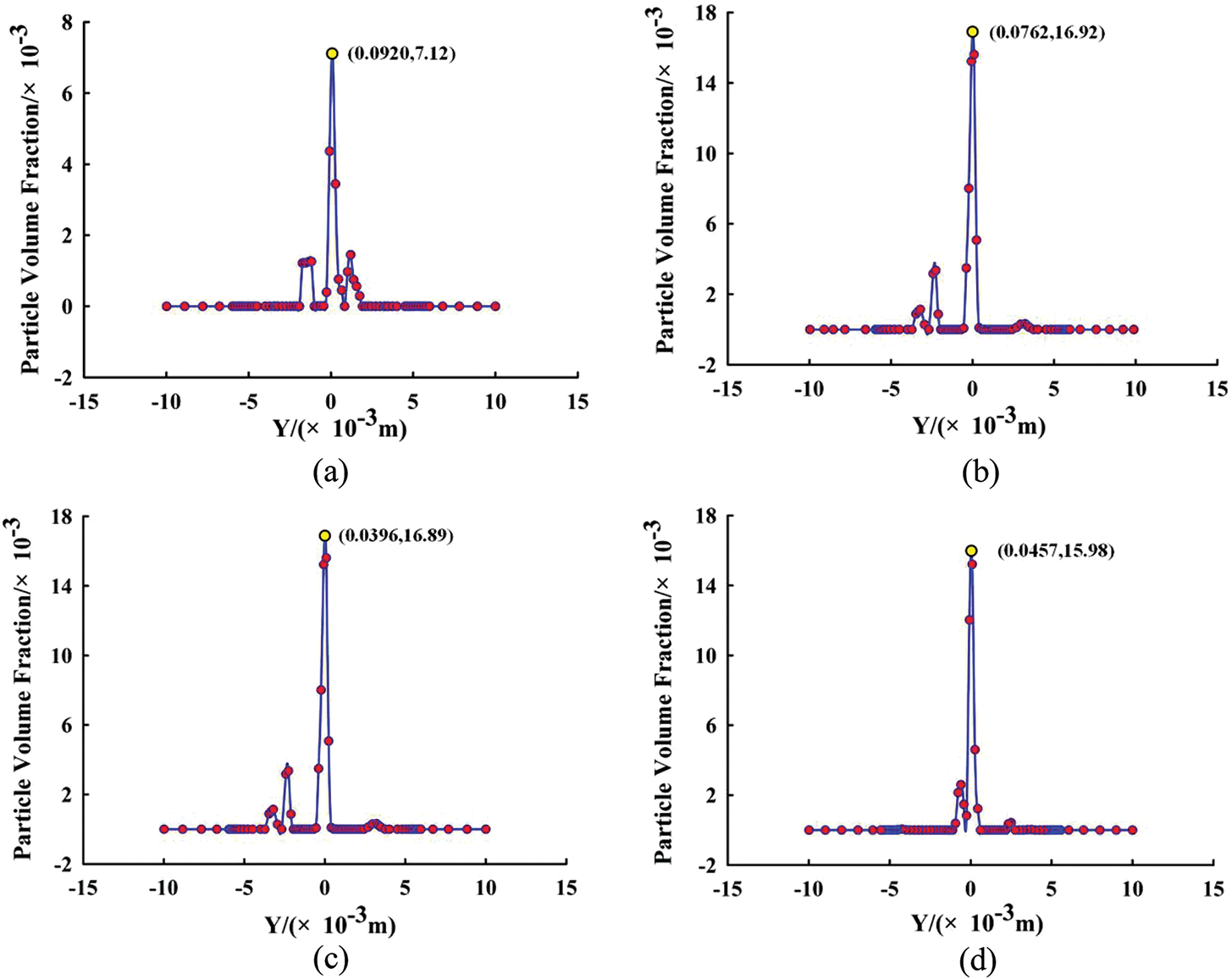
Figure 16: Dust flow concentration distribution per unit volume at different incident angles. (a) θ = 0°. (b) θ = 30°. (c) θ = 60°. (d) θ = 90°
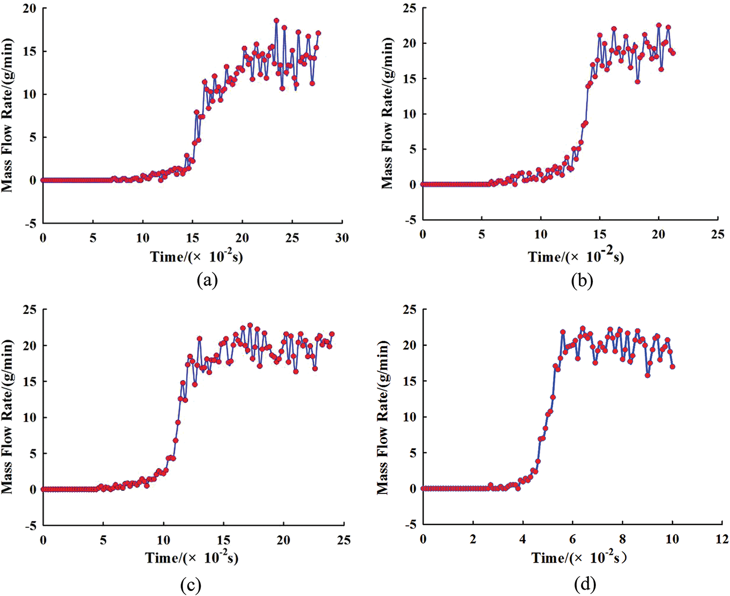
Figure 17: Mass flow rates of nozzle outlet at different powder injection angles. (a) θ = 0°. (b) θ = 30°. (c) θ = 60°. (d) θ = 90°
From the above simulation results, it can be seen that θ is an important factor. When θ is within the range of 0°–30°, the focus point of the powder flow will move upward as θ increases. The powder flow concentration per unit volume at the upper focus is smaller than the powder flow concentration per unit volume at the lower focus. When θ of the powder flow is within the range of 30°–90°, the focus point will move down as θ increases. When θ is 0°, the powder distribution is the most uniform. The number of collisions between the powder and the wall is too high, which causes some powder particles to rebound, and the mass flow rate of the powder flow from the nozzle is much lower than the powder feeding rate. When θ is 30°, the powder spatial distribution is more uniform than when θ is 60°. Due to the rebound of some particles, the mass flow rate at the nozzle outlet is slightly lower than the actual powder feeding rate. When θ is 30°, the powder flow concentration per unit volume at the focal point reaches the highest value, and the powder flow has the best agglomeration. When θ is 90°, the inlet and outlet of the nozzle basically reach the conservation of mass, where the mass flow rate balance time is the shortest and the powder flow utilization rate is the highest.
A smaller δ value not only increases the ejection speed of the gas and powder flow but also reduces the diameter of the powder flow concentration distribution. δ can effectively improve powder flow agglomeration. As δ increases, the powder flow concentration per unit volume at the nozzle focal point increases first and then decreases. When δ is 1.00 mm, the powder flow concentration per unit volume at the focal point is maximal, and the powder flow convergence is optimal. However, a δ value that is too small will cause a large number of powder particles to gather at the nozzle outlet, causing the concentration of the unit volume of the powder flow at the focal point to decrease.
The powder flow concentration per unit volume decreases as α increases, the focal length of the powder flow at the nozzle outlet becomes larger, and the focal concentration distribution diameter becomes larger. An excessively small α value will result in a larger divergence angle of the powder flow. An excessively large α value will cause the concentration distribution diameter of the unit volume of the powder flow at the focal point to be too large. When the concentration distribution diameter is larger than the diameter of the spot, the powder flow utilization rate is reduced.
When θ is less than 90°, the nozzle outlet mass flow rate will be lower than the actual mass flow rate. When θ is 90°, the nozzle outlet mass flow rate is the same as the inlet mass flow rate after stabilization. The nozzle inlet and outlet basically reach the conservation of mass, and the mass flow rate balance time is the shortest, thereby improving the utilization rate of powder flow. When θ is 30°, the powder flow concentration per unit volume at the focal point reaches its highest value, and the powder flow has the best agglomeration.
This paper analyses the influence of three different structural parameters of the coaxial powder feeding nozzle on powder flow agglomeration from a single-factor point of view. Research on powder flow agglomeration under the coupling effect of various parameters has not been previously carried out. The powder flow agglomeration of the coaxial powder feeding nozzle under the combined action of different structural parameters needs further analysis. In addition, how to find the optimal structural parameters to effectively improve the powder utilization rate on the basis of the constructed laser coaxial powder feeding nozzle DEM-CFD gas-powder two-phase flow model needs further analysis. Therefore, based on the coupling of various parameters, the model has a certain generalization ability, and an optimization model of a laser coaxial powder feeding nozzle structure parameter with an optimal powder utilization rate as the main optimization goal will be the focus of future efforts.
Funding Statement: This research is supported by the National Natural Science Foundation of China (Project No. 51675226), Natural Science Foundation of Liaoning Province (Project No. 20180550167) and Key Projects of Liaoning Province (Project Nos. LJ2017ZL001, LJ2019ZL005).
Conflicts of Interest: The authors declare that they have no conflicts of interest to report regarding the present study.
1. Haeri, S., Wang, Y., Ghita, O., Sun, J. (2017). Discrete element simulation and experimental study of powder spreading process in additive manufacturing. Powder Technology, 306(4), 45–54. DOI 10.1016/j.powtec.2016.11.002. [Google Scholar] [CrossRef]
2. Fiorineschi, L., Carfagni, M., Furferi, R., Governi, L., Rotini, F. (2018). The role of additive technologies in the prototyping issues of design. Rapid Prototyping Journal, 24(7), 1101–1116. DOI 10.1108/RPJ-02-2017-0021. [Google Scholar] [CrossRef]
3. Sing, S. L., An, J., Yeong, W. Y., Wiria, F. E. (2016). Laser and electron-beam powder-bed additive manufacturing of metallic implants: A review on processes, materials and designs. Journal of Orthopaedic Research, 34(3), 369–385. DOI 10.1002/jor.23075. [Google Scholar] [CrossRef]
4. Pu, Y. S., Wang, B. Q., Zhang, L. G. (2018). Metal 3D printing technology. Surface Technology, 47(3), 78–84. [Google Scholar]
5. Lee, H., Lim, C. H. J., Low, M. J., Tham, N., Kim, Y. J. (2017). Lasers in additive manufacturing: A review. International Journal of Precision Engineering and Manufacturing-Green Technology, 4(3), 307–322. DOI 10.1007/s40684-017-0037-7. [Google Scholar] [CrossRef]
6. Wang, H. M., Zhang, S. Q., Wang, X. M. (2009). Progress and challenges of laser direct manufacturing of large titanium structural components. Chinese Journal of Lasers, 36(12), 3204–3209. DOI 10.3788/CJL20093612.3204. [Google Scholar] [CrossRef]
7. Syed, W. U. H., Pinkerton, A. J., Li, L. (2006). Combining wire and coaxial powder feeding in laser direct metal deposition for rapid prototyping. Applied Surface Science, 252(13), 4803–4808. DOI 10.1016/j.apsusc.2005.08.118. [Google Scholar] [CrossRef]
8. Khamidullin, B. A., Tsiviilskkiy, I. V., Gorunov, A. I., Gilmutdinov, A. K. (2019). Modeling of the effect of powder parameters on laser cladding using coaxial nozzle. Surface and Coatings Technology, 364(9), 430–443. DOI 10.1016/j.surfcoat.2018.12.002. [Google Scholar] [CrossRef]
9. Peng, Y., Zhao, K., Yang, Y., Pu, H., Luo, J. (2019). Highly precise and efficient powder feeding system based on gravimetric feedback. Powder Technology, 354(1), 719–726. DOI 10.1016/j.powtec.2019.06.043. [Google Scholar] [CrossRef]
10. Kovalenko, V., Yao, J. H., Zhang, Q. L., Anyakin, M., Hu, X. D. et al. (2016). Development of multichannel gas-powder feeding system coaxial with laser beam. Procedia CIRP, 42, 96–100. DOI 10.1016/j.procir.2016.02.197. [Google Scholar] [CrossRef]
11. Pekkarinen, J., Salminen, A., Kujanp, V., Ilonen, J., Lensu, L. et al. (2016). Powder cloud behavior in laser cladding using scanning optics. Journal of Laser Applications, 28(3), 032007–032012. DOI 10.2351/1.4947598. [Google Scholar] [CrossRef]
12. Bi, G., Schürmann, B., Gasser, A., Poprawe, R. (2007). Development and qualification of a novel laser-cladding head with integrated sensors. International Journal of Machine Tools and Manufacture, 47(3–4), 555–561. DOI 10.1016/j.ijmachtools.2006.05.010. [Google Scholar] [CrossRef]
13. Liu, H., He, X. L., Gang, Y., Wang, Z. B., Zheng, C. Y. et al. (2015). Numerical simulation of powder transport behavior in laser cladding with coaxial powder feeding. Science China, 58(10), 104701–104710. [Google Scholar]
14. Wang, W., Cai, L., Yang, G., Bian, H. Y., Wang, G. et al. (2012). Research on the coaxial power feeding nozzle for laser cladding. Chinese Journal of Lasers, 39(4), 1–7. [Google Scholar]
15. Park, J., Chuang, S., Yun, H. Y., Cho, K., Chuang, C. et al. (2006). Asymmetric nozzle structure for particles converging into a highly confined region. Current Applied Physics, 6(6), 992–995. DOI 10.1016/j.cap.2005.07.004. [Google Scholar] [CrossRef]
16. Liang, B. J., Gao, D. R., Wu, S. F., Li, Y. H. (2016). Influence of key structure parameters on the descaling nozzle performance. Chinese Hydraulics & Pneumatics, 6, 6–29. [Google Scholar]
17. Wachem, B. G. M. V., Schouten, J. C., Bleek, C. M., Krishna, R., Sinclair, J. L. (2001). Comparative analysis of CFD models of dense gas–solid systems. AIChE Journal, 47(5), 1035–1051. DOI 10.1002/aic.690470510. [Google Scholar] [CrossRef]
18. Gopireddy, S. R., Hildebrandt, C., Urbanetz, N. A. (2016). Numerical simulation of powder flow in a pharmaceutical tablet press lab-scale gravity feeder. Powder Technology, 302, 309–327. DOI 10.1016/j.powtec.2016.08.065. [Google Scholar] [CrossRef]
19. Deen, N. G., Annaland, M. V. S., Hoef, M. A. V., Kuipers, J. A. M. (2007). Review of discrete particle modeling of fluidized beds. Chemical Engineering Science, 62(1–2), 28–44. DOI 10.1016/j.ces.2006.08.014. [Google Scholar] [CrossRef]
20. Zhang, J., Yang, L., Zhang, W., Qiu, J. B., Xiao, H. B. et al. (2020). Numerical simulation and experimental study for aerodynamic characteristics and powder transport behavior of novel nozzle. Optics and Lasers in Engineering, 126(3), 105873. DOI 10.1016/j.optlaseng.2019.105873. [Google Scholar] [CrossRef]
21. Gao, J. L., Wu, C. Z., Liang, X. D., Hao, Y. B., Zhao, K. (2020). Numerical simulation and experimental investigation of the influence of process parameters on gas-powder flow in laser metal deposition. Optics & Laser Technology, 125(1–2), 106009. DOI 10.1016/j.optlastec.2019.106009. [Google Scholar] [CrossRef]
22. Fries, L., Antonyuk, S., Hrinrich, S., Dopfer, D., Palzer, S. (2013). Collision dynamics in fluidised bed granulators: A DEM-CFD study. Chemical Engineering Science, 86(3), 108–123. DOI 10.1016/j.ces.2012.06.026. [Google Scholar] [CrossRef]
23. Suri, Y., Islam, S. Z., Hossain, M. (2020). Numerical modelling of proppant transport in hydraulic fractures. Fluid Dynamics & Materials Processing, 16(2), 297–337. DOI 10.32604/fdmp.2020.08421. [Google Scholar] [CrossRef]
24. Zhou, H., Gao, H., Fang, Z., Yng, J., Wu, M. (2020). Analysis of gas-solid flow characteristics in a spouted fluidized bed dryer by means of computational particle fluid dynamics. Fluid Dynamics & Materials Processing, 16(4), 813–826. DOI 10.32604/fdmp.2020.010150. [Google Scholar] [CrossRef]
25. Levy, A., Brosh, T. (2010). Modeling of heat transfer in pneumatic conveyer using a combined DEM-CFD numerical code. Drying Technology, 28(2), 155–164. DOI 10.1080/07373930903517482. [Google Scholar] [CrossRef]
26. Al-Arkawazi, S., Marie, C., Benhabib, K., Coorevits, P. (2016). Modeling the hydrodynamic forces between fluid-granular medium by coupling DEM-CFD. Chemical Engineering Research and Design, 117(1), 439–447. DOI 10.1016/j.cherd.2016.11.002. [Google Scholar] [CrossRef]
27. Heynderickx, G. J., Das, A. K., Wilde, J. D., Marin, G. B. (2004). Effect of clustering on gas-solid drag in dilute two-phase flow. Industrial & Engineering Chemistry Research, 43(16), 4635–4646. DOI 10.1021/ie034122m. [Google Scholar] [CrossRef]
28. Vandewalle, L. A., Gonzalez, Q. A., Perreault, P., Geem, K. M. V., Marin, G. B. (2019). Process intensification in a gas–solid vortex unit: CFD model based analysis and design. Industrial & Engineering Chemistry Research, 58(28), 12751–12765. DOI 10.1021/acs.iecr.9b01566. [Google Scholar] [CrossRef]
29. Chien, C. H., Theodore, A., Wu, C. Y., Hsu, Y. M., Birky, B. (2016). Upon correlating diameters measured by optical particle counters and aerodynamic particle sizers. Journal of Aerosol Science, 101(1), 77–85. DOI 10.1016/j.jaerosci.2016.05.011. [Google Scholar] [CrossRef]
30. Roth, G. A., Aydogan, F. (2015). Derivation of new mass, momentum, and energy conservation equations for two-phase flows. Progress in Nuclear Energy, 80, 90–101. DOI 10.1016/j.pnucene.2014.12.007. [Google Scholar] [CrossRef]
31. Ali, A., Kalisch, H. (2014). On the formulation of mass, momentum and energy conservation in the KdV equation. Acta Applicandae Mathematicae, 133(1), 113–131. DOI 10.1007/s10440-013-9861-0. [Google Scholar] [CrossRef]
32. Feng, S., Xiong, D., Chen, G., Cui, Y., Chen, P. (2020). Convection-diffusion model for radon migration in a three-dimensional confined space in turbulent conditions. Fluid Dynamics & Materials Processing, 16(3), 651–663. DOI 10.32604/fdmp.2020.07981. [Google Scholar] [CrossRef]
33. Jonsson, V. K., Sparrow, E. M. (1966). Experiments on turbulent-flow phenomena in eccentric annular ducts. Journal of Fluid Mechanics, 25(1), 65–86. DOI 10.1017/S0022112066000053. [Google Scholar] [CrossRef]
34. Eric, S., Fazel, H. (2016). External turbulence-induced axial flow and instability in a vortex. Journal of Fluid Mechanics, 793, 353–379. DOI 10.1017/jfm.2016.123. [Google Scholar] [CrossRef]
35. Wilcox, D. C. (2008). Formulation of the k-ω turbulence model revisited. AIAA Journal, 46(11), 2823–2838. DOI 10.2514/1.36541. [Google Scholar] [CrossRef]
 | This work is licensed under a Creative Commons Attribution 4.0 International License, which permits unrestricted use, distribution, and reproduction in any medium, provided the original work is properly cited. |